Two-Area Automatic Generation Control for Power Systems with Highly Penetrating Renewable Energy Sources

Abstract

Currently, renewable energy sources (RESs) are gradually replacing traditional power sources that use fossil fuels. In some countries, such as Vietnam, RESs are developed on a massive scale and are concentrated in some key areas. This causes negative impacts on a power system when its transmission system is not deployed synchronously to release their capacity from these new renewable energy plants. An important challenge today is to ensure frequency stability in power systems with high uncertainty in RES output power. Additionally, the system requires solutions to prevent transmission line overloads during periods when RESs make a substantial contribution to the electricity generation capacity. Therefore, this paper builds an automatic generation control (AGC) system for a two-area power system with high penetration of RESs. This AGC system model aims to maintain system frequency stability amid unpredictable changes in RESs while also ensuring that tie-lines transmit the predetermined power levels to mitigate frequent congestion. By continuously monitoring and adjusting the system’s frequency, the challenges posed by the inherent variability of RESs can be effectively mitigated. The AGC model is simulated on DIgSILENT PowerFactory software and tested with a 106-bus system. The simulation results of this study show that the AGC system operates effectively, ensuring that the frequency returns to the rated value and maintaining the exchange capacity on the tie-lines after occurrences of RES power decrease events.

1. Introduction

Today, the development of RESs is an inevitable development direction for countries around the world. Limiting fossil fuel use and reducing greenhouse gas emissions are the main drivers for the development of RESs. In 2023, the global annual increase in renewable energy capacity soared by almost $50\%$, reaching nearly 510 gigawatts (GW); this is the highest growth rate seen in the last twenty years [1]. According to the International Energy Agency (IEA), with current policies and market conditions, global renewable energy capacity is expected to reach 7300 GW by 2028. This growth trend shows that, by 2030, global renewable energy capacity will increase by 2.5 times compared to today [1]. Contributing largely to this increase is the deployment of solar and wind energy systems, which replace traditional energy sources. According to the IEA, among ASEAN countries, Vietnam has the highest level of renewable energy deployment. Solar and wind power capacity in Vietnam increased from nearly 0 in 2017 to more than 22 GW in 2021, thanks to the implementation of feed-in tariffs [2]. Vietnam has the potential to develop RESs including 963 GW of solar power and 821 GW of wind power; of this, the onshore wind power potential is 221 GW and the offshore wind power potential is 600 GW [3]. In Vietnam, although the development of RESs is being strongly encouraged throughout the country, it is only concentrated in a few key regions, such as the Central Highlands, the South Central Coast, the Southeast, and the Southwest regions. These are the areas with the highest solar radiation levels in Vietnam and they are presently the focus for investments in large-capacity solar power plants and wind power plants. Regional RESs serve local loads and transmit electricity to other regions. Although these new RESs help in increasing Vietnam’s total power capacity and contribute a significant amount of electricity to the system, they cause some difficulties in operating the power systems.

The rapid massive development and concentration of large-capacity RESs in some key areas have caused several negative impacts on Vietnam’s electricity system. The Central Highlands and South Central regions have relatively low loads, which causes excess electricity and puts great pressure on the transmission system. Moreover, the transmission system has not yet developed sufficiently to keep pace with the rapid growth rate of RESs. This causes a number of bad conditions in the electrical system, including the overloading of electrical equipment, local overvoltage [4], voltage instability [5], harmonics [6], protection relays [7], and low system inertia [8]. In particular, the uncertainty of RESs causes many difficulties in the operation of power systems. The issue of maintaining system frequency stability under the high penetration of RESs with fluctuating output power is currently a significant concern. When solar power generates large amounts of electricity during the day, traditional sources (thermal and hydroelectric) are forced to cut capacity so the system can absorb excess renewable energy. This causes the inertia in the power system to be greatly reduced, easily causing frequency instability and transient response phenomena.

In addition, in some areas (such as Vietnam), power systems with an excessive concentration of RESs in some key areas can easily become unstable when the RES capacity fluctuates abnormally. Just a change in input factors—such as a change in solar radiation, a change in wind source, or an unexpected incident—can cause a capacity shortage in the system, causing the frequency to change and the power to fluctuate. The phenomenon of clouds covering solar panels on a large scale occurs frequently and changes rapidly, causing a constant power imbalance in the system. Therefore, an AGC controller needs to be set up to maintain frequency stability against RES fluctuations. A traditional generator with fast response capabilities, such as hydro power, needs to be connected to this AGC system to take on the role of frequency regulation [9].

The frequency of the electrical system is controlled by the AGC system through two control loops—the primary and secondary loops, respectively. The primary control loop comprises the operation of the governor at generators with droop characteristics to keep the frequency from fluctuating strongly, minimizing the frequency’s steady-state error. The AGC system’s secondary control loop, also known as the load frequency control (LFC), regulates the generator output power to return the frequency to the nominal value within an acceptable margin. The popular AGC algorithm uses a linear equation called the area control error $\left(ACE\right)$ equation as a monitoring signal to effectively regulate the frequency [9]. The variables in the equation of $ACE$ include the frequency change during disturbance events and the power exchanged between single/multiple areas. The purpose of the AGC is to promptly stabilize frequency and power deviations on the tie-line which have occurred because of load or power fluctuations. This AGC system is essential today because RES uncertainty continuously causes power imbalance in the power system.

The authors of [10,11] review in detail the up-to-date studies on AGC/LFC for both conventional- and renewable-energy-based power systems. The authors not only present an in-depth review of the types of power system models—divided into single-area and multi-area models—but they also analyze the control methods of the current AGC system. The AGC system can use traditional control models such as PI/PID [12,13] or advanced controllers such as a fuzzy logic controller [14], an artificial neural network [15], or particle swarm optimization [16,17]. In addition, the authors of [18] also present a detailed review of the advantages, disadvantages, and improvements that have been made in LFC technologies. In general, the current improved methods have all been developed based on traditional linear PI controllers. These are considered to be the basic controllers in the current AGC systems. In [10], the AGC control system is also studied with regard to many concepts in the context of high-penetration RESs [19] and that of other aspects such as AGC combined with distributed generators [20] and AGC of a multi-source system in a smart grid [21] and in a microgrid [22]. Here, the authors also emphasize that there is currently still a lack of research about AGC systems with deeper penetration of RESs. In [23], the authors examine the future frequency stability of the KSA power system with high RES penetration. However, their analysis only considers system frequency stability in scenarios involving simple generator losses and does not include the development of an AGC system to restore the frequency to its nominal value. In [17], the authors develop an LFC model for a three-area interconnected power system incorporating renewable energy. This model uses linear active disturbance rejection control and employs an improved particle swarm optimization algorithm for parameter optimization. The results demonstrate that the enhanced controller significantly reduces both system frequency and line exchange power deviation. However, the study does not include experiments on scenarios involving instantaneous power changes in RES, nor does it establish a unified AGC/LFC model for frequency regulation across all three areas of the power system.

The above analysis highlights the research gap in constructing AGC systems that are designed to handle unpredictable changes in RESs, especially in power systems where RESs make up a substantial portion of the total capacity. In [10], the authors emphasize that there remains a lack of research about AGC systems with deeper penetrations of RESs. In addition, previous studies have primarily focused on control algorithms and tested simplistic scenarios. They also lack a thorough analysis of how system components behave under the operation of the AGC controller. Therefore, this study presents the design and simulation of an AGC system for a two-area power network within a 106-bus system characterized by high RES penetration. The AGC system is responsible for frequency regulation and maintaining the power exchange balance between Areas 1 and 2. It incorporates a PI control strategy along with the $ACE$ algorithm to achieve these objectives. The objectives of the AGC system are designed to ensure the following: (1) instantaneous power adjustment in response to decreases or increases in capacity from RESs; (2) the maintenance of frequency stability within permissible operating limits; (3) the maintenance of the transmission power on tie-lines at a predetermined value to prevent congestion between the two areas. This AGC control system is tested under two scenarios: (1) an immediate decrease in generating capacity of closely clustered solar power plants; (2) the forced shutdown of a critical traditional generator during the frequency adjustment process due to an operational issue. The contributions of this research include:

• Development of an AGC controller model for a 106-bus power system using DIgSILENT PowerFactory software [24]. This model integrates various power sources such as wind, solar, hydro, and thermal power, with RESs constituting a significant portion of the total generating capacity.
• Testing the AGC system under two scenarios involving instantaneous changes in RES capacity within the system. Scenario 1 is the process of reducing the generation capacity of RES on the grid and Scenario 2 considers the failure of an important generator participating in the AGC system during the frequency adjustment process. These scenarios are designed based on common events observed in practical operations.
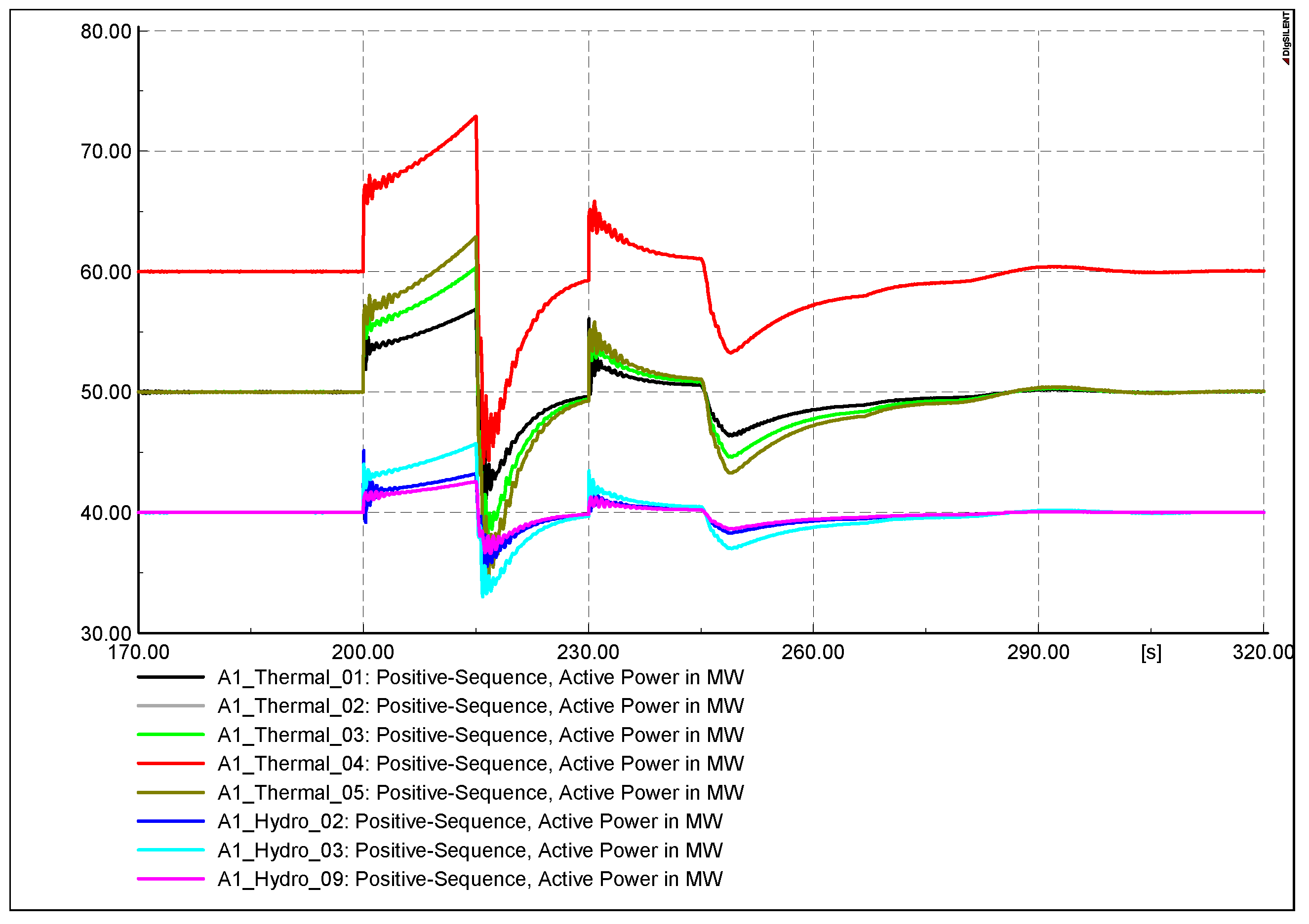
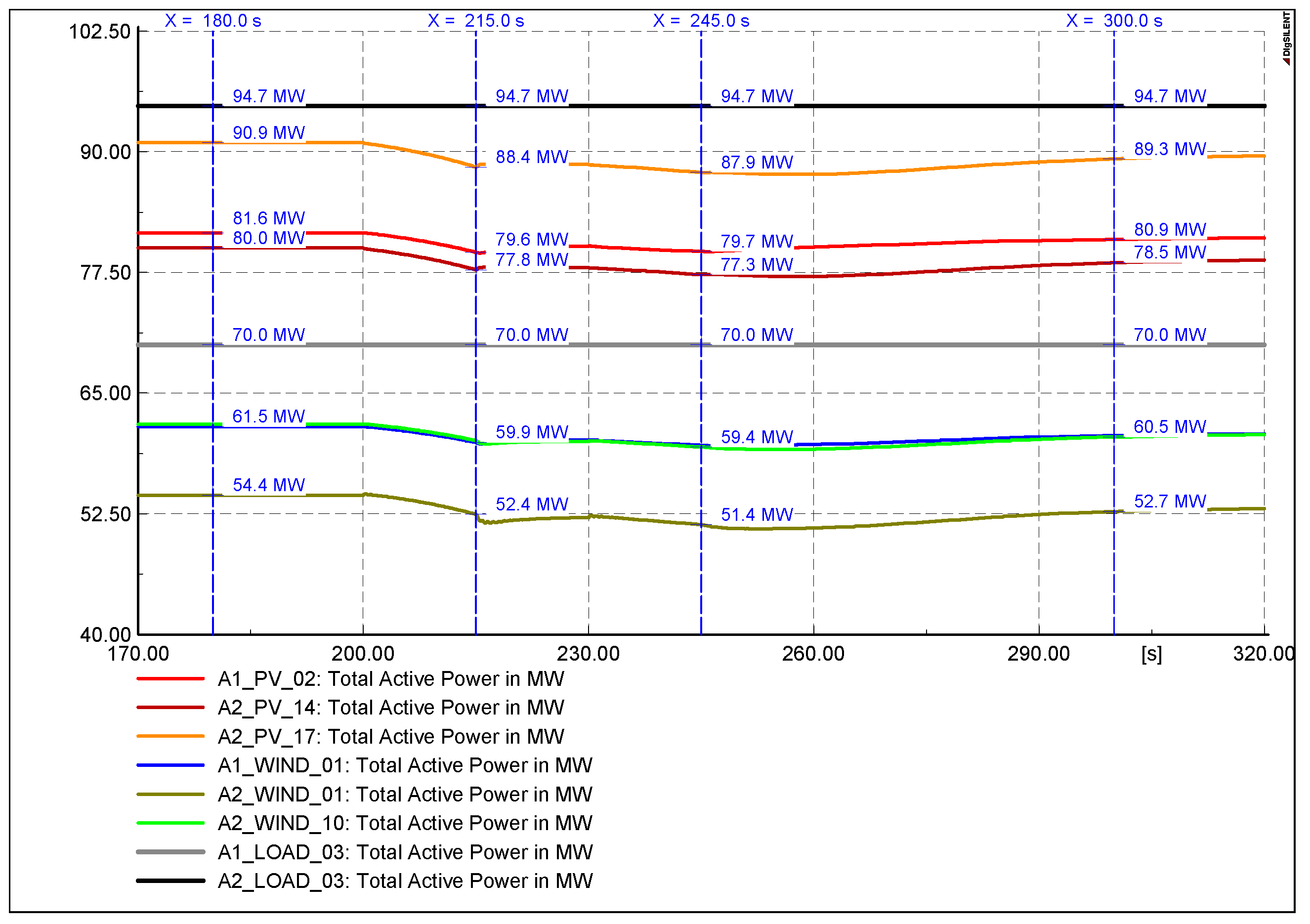
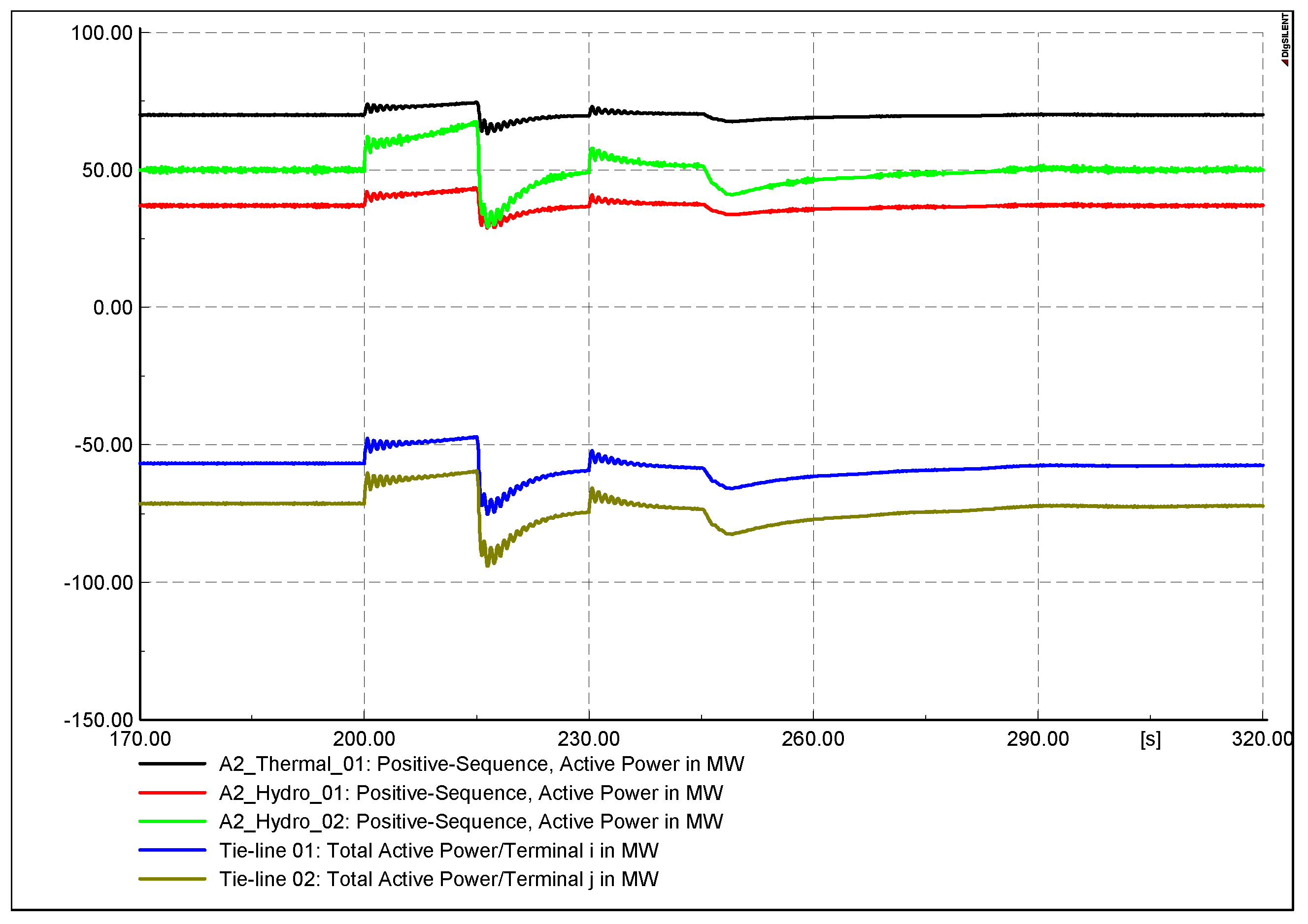
• Analyze the operation of traditional generators involved and not involved in the AGC system, as well as system frequency, power flow on tie-lines, and other elements within the power system.

The remaining part of this paper is organized as follows. Section 2 presents the two-area AGC model, including the transfer function model and the principle of power allocation between areas. Section 3 summarizes the power system characteristics to be applied in the case study. It also presents the simulation results and analysis. Finally, the main conclusions are summarized in Section 4.

2. Two-Area AGC Model

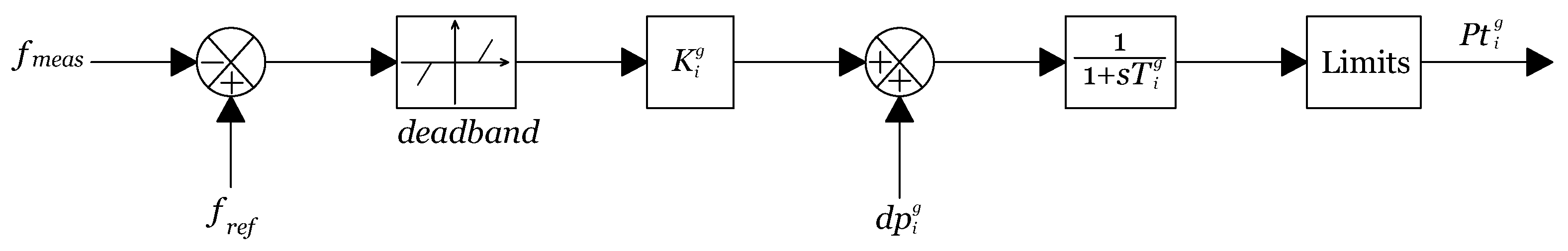
2.1. Turbine–Governor Control System

The governor is a system that automatically and instantaneously adjusts the rotation speed of the generator according to the frequency variation, contributing to the restoration of the frequency to the nominal frequency of the power system. The governor is equipped with the most hydroelectric- and thermal-power-generating sets in the simulation. The main effects of the governor include the following: (i) quickly curbing the imbalance between output power and load, with the ongoing the existence of a frequency deviation; (ii) changing the power flow in the system; (iii) the effectiveness of primary frequency regulation depends greatly on the damping characteristics. The smaller the slope (the same load change leads to a smaller rate of change), the greater the adjustment effect. If the droop characteristic is horizontal, it is called an isochronous governor, which ensures that the frequency does not change as the load changes until the turbine power limit is exhausted. This type of governor is only used in independent power grids with only one generator and is responsible for controlling the frequency. The governor droop characteristics are presented in Figure 1. Here, the x-axis presents the output power of generator (MW), while the y-axis shows the electrical frequency of the power system, Hz.

The turbine–governor controller is required to regulate the generating capacity of the generator through control signals. This will act on the valves/gates to change the mechanical power of the turbine, thereby changing the generating capacity of the generator. The main task of the governor is to maintain the generating capacity of the generator at a predetermined point value. Figure 2 shows the turbine–governor’s transfer function. It consists of the following signal: The measured system frequency $f_{meas}$ and the reference frequency $f_{ref}$ are compared to determine the frequency deviation (error signal). Then, if the error signal is outside the dead band, it is amplified by block $K_i^g$ and added with the secondary control signal $d{p}_i^g$ (generator g in area i), which is the AGC output. $K_i^g$ is the droop characteristic of each generator g in area i. It should be noted that, when the governor is in the first stage of the primary frequency control loop, the $d{p}_i^g$ has not been sent to the governor from the AGC system $\left(d{p}_i^g=0\right)$, the governor will immediately adjust the power of the generators so that the frequency does not decrease (or increase) too much. When the $d{p}_i^g$ signal is input, the governor will increase or decrease the power to meet the secondary frequency control loop. The requested power signal then passes through the turbine–governor’s characteristic set ${\displaystyle \frac{1}{1+s{T}_i^g}}$. The limit block is created to limit the power output of the turbine (the valve/gate of the fuel opening–closing value), with a value from 0 to 1. The output signal $P{t}_i^g$ is the generator’s capacity after adjustment [25].

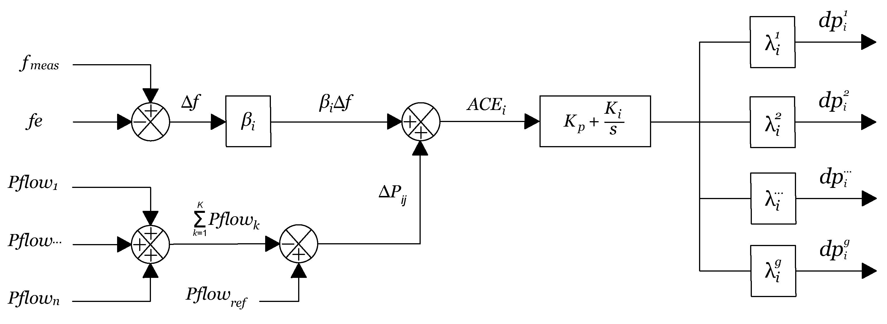
2.2. AGC Algorithm for Two-Area Power System

The AGC algorithm uses $ACE$ as a monitoring signal and sets it to zero in the event of changing the balance of the generation power and load on the system. The $ACE$ signal includes the deviations of the system frequency and the interchange power between the two areas. The algorithm aims to ensure that any power imbalance that occurs in a particular area of the power system is promptly corrected in that same area. Adjustment to return to power balance is performed by AGC secondary control in that area. Equations (1)–(3) present the expression of $ACE$ and the related elements:

$$\begin{array}{cc}\hfill & AC{E}_i=\Delta P_{ij}+{\beta }_i\Delta f\hfill \end{array}$$

(1)

$$\begin{array}{cc}\hfill & \Delta P_{ij}=\sum _{k=1}^{K}P flo{w}_k-P flo{w}_{ref}\hfill \end{array}$$

(2)

$$\begin{array}{cc}\hfill & \Delta f=f_{meas}-f_{ref}\hfill \end{array}$$

(3)

where $AC{E}_i$ is the area control error of area i, $\Delta P_{ij}$ is the tie-line power flow error between bus i and $j,{\beta }_i$ is the frequency bias coefficient of the area i, and $\Delta f$ is the frequency error of the power system. Equation (2) shows the interchange power deviation, where $P flo{w}_k$ is the exchange power on tie-line k and there is a total of K tie-lines connecting two areas. $P flo{w}_{ref}$ is the reference set of power exchange in the tie-lines. Equation (3) also presents the frequency error of the system, where $f_{meas}$ is the measurement frequency at the rotor and $f_{ref}$ is the nominal frequency of the system.

The AGC controller is applied to both areas and determines each $AC{E}_i$ value for each area including $AC{E}_1=\Delta P_{12}+{\beta }_1\Delta f$ and $AC{E}_2=\Delta P_{21}+{\beta }_2\Delta f$. Assuming that the decrease in the generating capacity of the power source within Area 1 causes frequency deviation, the generators in Area 1 have enough spinning reserves and will take on the task of returning the frequency to the nominal value $(AC{E}_1=0)$. The power adjustment at the generators is only made in Area 1, so there is no change in the Area 2 generation or tie-line flow. If the reserve capacity of Area 1 is not enough, then $AC{E}_1$ still exists, because $\Delta f$ is non-zero. At this time, the remaining $\Delta P_{12}$ and $\Delta f$ are switched by excess power from Area 2 to compensate for Area 1, helping to bring $AC{E}_1$ to 0. The frequency is stabilized at $f_{ref}$. The lack of power in Area 1 can be completely compensated for by the amount of power from Area 2. In essence, this controller can restore the frequency to a stable value of $f_{ref}$ if there is enough reserve power for the secondary control. The frequency will be stabilized thanks to the amount of power from one area supporting the other.

The proportional–integral (PI) of $AC{E}_i$ over a certain time interval in the Laplace domain is expressed by Equation (4):

$$\begin{array}{cc}\hfill & P_{AGC}\left(s\right)=\left(K_p+{\displaystyle \frac{K_i}{s}}\right)·AC{E}_i\left(s\right)\hfill \end{array}$$

(4)

The $P_{AGC}$ signal, after passing through the PI controller, will be multiplied by each participation coefficient of the generators in the AGC system $\left({\lambda }_i^g\right)$, finally obtaining the $d{p}_i^g$ signal sent to the governor of the generator g in area i:

$$\begin{array}{cc}\hfill & d{p}_i^g=P_{AGC}·{\lambda }_i^g\hfill \end{array}$$

(5)

$$\begin{array}{cc}\hfill & {\lambda }_i^g={\displaystyle \frac{P_{{max}_i}^g}{{\displaystyle \sum _g}{P}_{{max}_i}^g}}\hfill \end{array}$$

(6)

Equation (6) presents the usual method of determining the participation coefficient ${\lambda }_i^g$ of the generators in the AGC system. It is usually chosen according to the ratio between the maximum power of the generator g ($P_{{max}_i}^g$) and the total maximum power of the generators participating in the secondary frequency modulation (${\displaystyle \sum _g}{P}_{{max}_i}^g$). However, this method will not ensure the amount of frequency control capacity when power imbalance events continuously occur in the system. Therefore, the chosen ${\lambda }_i^g$ coefficients of the generators should be larger than the value calculated by Equation (6) and less than 1 to reduce the transients of the generators.

The transfer function of the AGC system and the composite model are represented in Figure 3 and Figure 4, respectively.

3. Result and Analysis

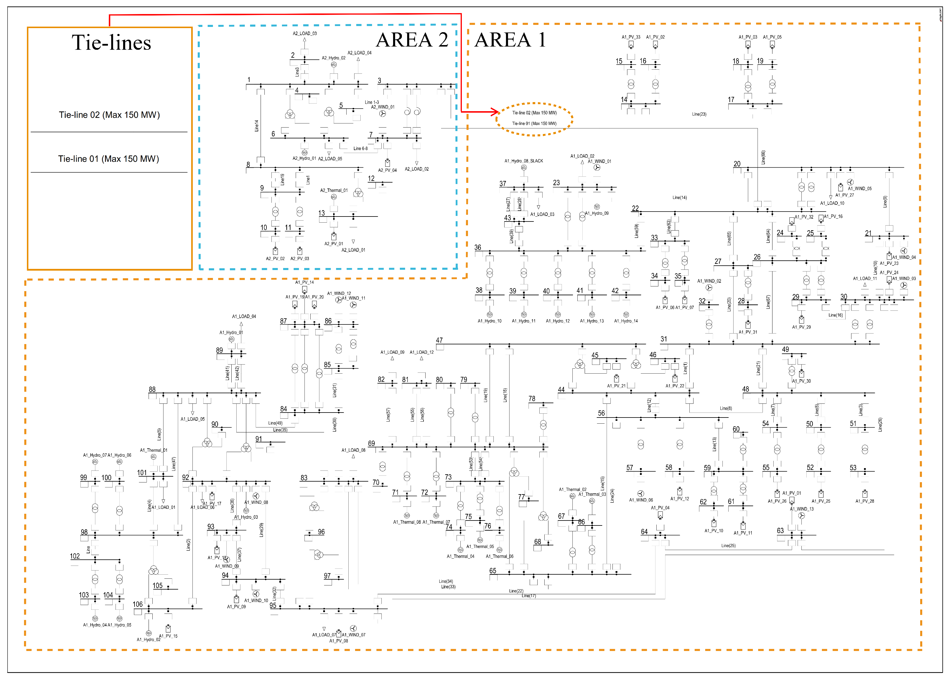
3.1. Network Overview

In this study, a 106-bus system—shown in Figure 5—with a high concentration of RESs is used to test the AGC model. The test case is a simple network with centrally developed RESs based on the Vietnam Electricity Development Plan for the period 2021–2030 [3]. The system includes 106 buses, with voltage levels up to 220 kV, and 61 transmission lines, divided into two areas, i.e., Areas 1 and 2, connected through 2 tie-lines. The principle of area division is based on two main factors: (i) geographical distribution and (ii) congestion of lines. The two areas in the case study are geographically divided and are connected through two tie-lines that are frequently congested. The total transmission capacity of these tie-lines is 300 MW. The system includes 9 thermal power plants and 16 hydropower plants with total rated capacities of 4160 MW and 2400 MW, respectively; there are 37 solar power plants and 14 wind power plants which have total rated capacities of 1990 MW and 630 MW, respectively.

Table 1. Areas 1 and 2 system data.

	Area 1		Area 2
	No.	Rate Capacity [MW]	No.	Rate Capacity [MW]
Transmission lines	54	_	6	_
Transmission tie-lines	02	300	02	300
Thermal power plant	08	3950	01	210
Hydropower plant	14	1950	02	450
Wind power plant	13	570	01	60
Solar power plant	33	1800	04	190

summarizes the data of two areas of the 106-bus power system. We assume that the system is calculated at noon when the power output of the RESs is generated at the rated capacity, which is 2620 MW. To exploit the maximum amount of electricity from renewable energy plants, thermal and hydroelectric plants are required to generate at a low capacity about of 1060 MW. RESs account for about 70% of the total generated capacity of the power system; the rest is from traditional power sources. The load of the power system is assumed to be relatively low at 12:00 noon with a total capacity of 2640 MW, with characteristics far from the power source locations. The excess power is assumed to be transmitted to other systems via the slack bus, located in Area 1, with a transmission capacity of around 900 MW. The simulation and calculation of the AGC control system are performed using DIgSILENT PowerFactory software.

The generators assigned for frequency control include the following: (i) Area 1—A1_Hydro_01, A1_Hydro_04, A1_Hydro_05, A1_Hydro_06, and A1_Hydro_07; (ii) Area 2—A2_Hydro_01 and A2_Hydro_02. These generators are responsible for both primary and secondary frequency-regulation processes. The remaining hydroelectric and thermal generators only participate in the first phase of primary frequency regulation through their governors (within the first 15 s to keep the frequency from changing too quickly). The total fast response reserve capacity for frequency control of Areas 1 and 2 is 521 MW and 325 MW, respectively. In addition, the amount of spare capacity of thermal power plants operating at minimum capacity is 3470 MW; the total amount from the hydropower plants that do not participate in frequency regulation is 430 MW. This is an assumed amount of capacity that does not guarantee rapid system response and must be required by dispatch command.

The working sequence of the governor and the AGC system is simulated according to the principles of the circular regulating Vietnam’s electricity transmission system [26]. When the frequency deviates from the dead band of the speed-regulation system, the generators participating in primary frequency control must meet at least 50% of the primary frequency control capacity in the first 15 s, and must meet 100% in the first 30 s. Then, this power level must be maintained for at least the next 15 s. After 45 s following the event, the AGC controller sends $d{p}_i^g$ signals to the generators to perform secondary frequency control, bringing the frequency to 50 Hz. Generators equipped with a governor but not required to participate in frequency control only respond according to the slope characteristic within the first 15 s of the event.

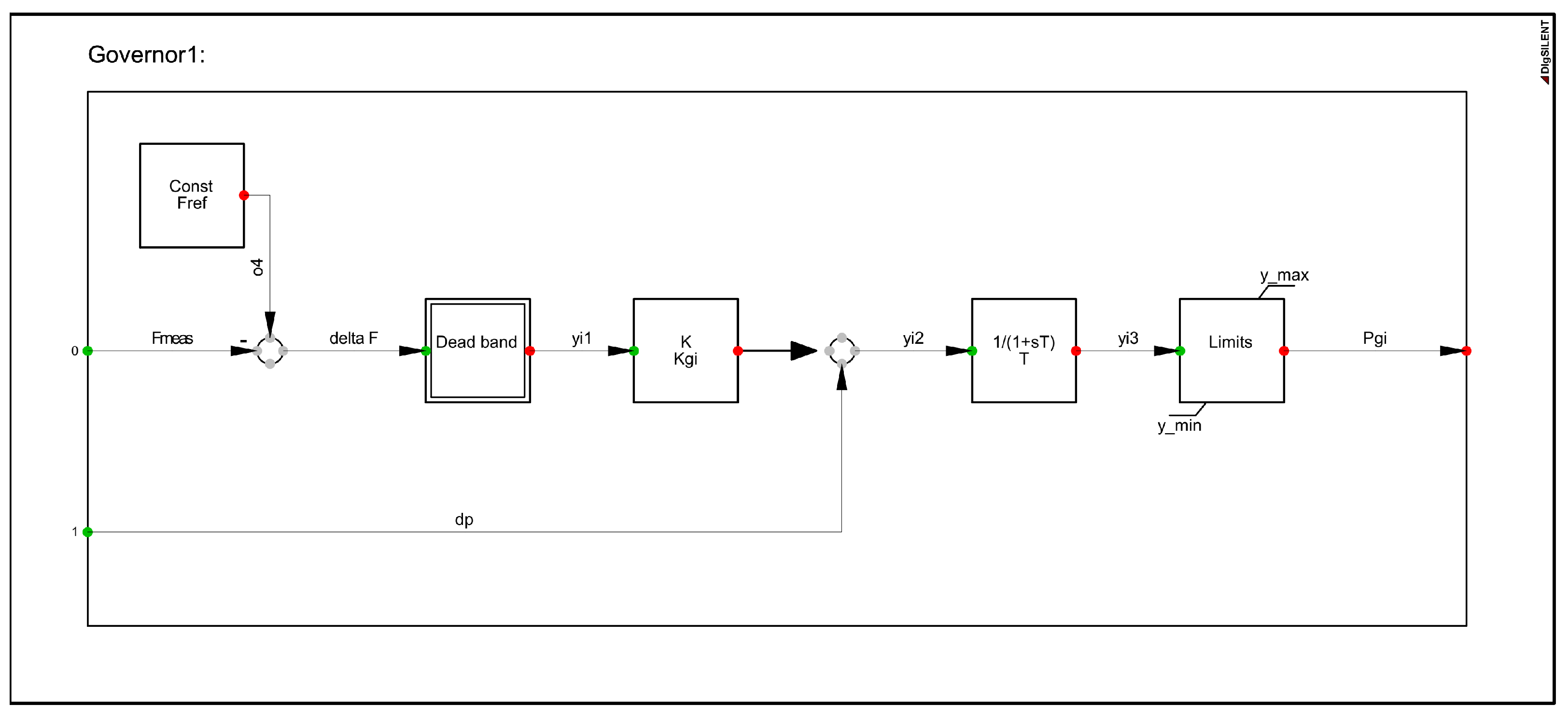
3.2. Governor and AGC Model in DIgSILENT PowerFactory

The article builds its own turbine–governor controller model on the DIgSILENT PowerFactory software based on the transfer function principle presented in Section 2.1. This control model in the software is presented in Figure 6. In particular, $f_{ref}$ is a reference system with a set value of 50 Hz. $f_{meas}$ is the system frequency measured. The control parameters include $K_i^g$, which is the droop characteristic, and the governor time constant is $T_i^g$. In this paper, the droop characteristic of all generators is set to $5\%$, corresponding to $K_i^g=20$. According to [25,27], $T_i^g$ is recommended to be in the range from 0.02 to 0.2 s for a steam turbine–governor, and in the range from 0.5 to 10 s for a hydro turbine generator. In this paper, $T_i^g$ of steam turbine–governors are set to 0.1 s and the hydro turbine generators are set to 1 s. The dead bands of all the governors are set to 0.05 Hz. In addition, for generators participating in the frequency controller, there will be an additional $d{p}_i^g$ signal from the AGC controller. Generators that do not participate in the frequency regulation have this signal removed from the governor. Solar and wind generators use dynamic models that are available in the software.

Table 2. Parameters set on the turbine–governor controller.

Block	Represent	Value
$f_{ref}$	Reference frequency	50
Dead band	Dead band of governor	0.05
$K_i^g$	Inverse droop	20
$T_i^g$	Governor time constant	Hydro turbine: 1 Steam turbine: 0.1
Limits	Limits turbine capacity	y _max: 1 y _min: 0

summarizes the parameters set on the turbine–governor controller in this study.

This study also built a novel AGC controller model on DIgSILENT PowerFactory based on the operating principles presented in Section 2.2. The AGC controller for Area 1 is shown in Figure 7 (similar to the controller AGC for Area 2 with a corresponding number of generators). In particular, $f_{ref}$ is a reference system with a set value of 50 Hz. $f_{meas}$ is the measurement frequency measured from the system. Additionally, $P flo{w}_1$ and $P flo{w}_2$ are the powers measured on the two tie-lines of the 106-bus system. $P flo{w}_{ref}$ is the power allowed for transmission on these two tie-lines and is set to 125 MW. Block Const lambda (${\lambda }_i^g$) are the participation coefficients of frequency-modulated generators in the area. In Area 1, the participation coefficient of the five generators is set to 0.6, except for generator A1_Hydro_01, which has the largest adjustment ability and which is set to 0.8. In Area 2, two generators—A2_Hydro_01 and A2_Hydro_02—have a participation coefficient of 0.6. The constant bias block represents the frequency bias of the area; for Areas 1 and 2, this is set to be 25 and 20 MW/0.1 Hz, respectively. The PI controller is characterized by two coefficients $K_p$ and $K_i$, which affect the controller’s stability. In this paper, the PI controller has been calibrated through many rounds of testing to obtain the appropriate parameters: $K_p=0.5,K_i=100$ for both Areas 1 and 2.

Table 3. Parameters set on the AGC controller in two both area.

Block	Represent	Value
		Area 1	Area 2
$f_{ref}$	Reference frequency	50	50
Constant Bias	Frequency bias	25	20
$Pflo{w}_{ref}$	Preset power area exchange	125	125
$K_p$	$K_p$ in PI controller	0.5	0.5
$K_i$	$K_i$ in PI controller	100	100
${\lambda }_i^g$	Participation coefficient of generator g in area i	0.6 (0.8 for A1_Hydro_01)	0.6

summarizes the parameters set on the AGC controller in both areas.

3.3. Simulation Results

The article proposes two scenarios on which to test the performance of the AGC model with a high penetration of RESs. The scenarios are built to occur in Area 1, where there is a proportion of RESs in the total generating capacity of all power sources. Scenario 1 is an event where the capacity of solar power plants in Area 1 decreases due to cloud cover. Scenario 2 is more complicated than Scenario 1; here, two consecutive events will occur during the frequency adjustment process. First, the capacity of the RESs in Area 1 suddenly drops due to cloud cover, but the AGC system will work. Next, during the frequency adjustment process, a generator set responsible for controlling the frequency in Area 1 fails, forcing it to shut down.

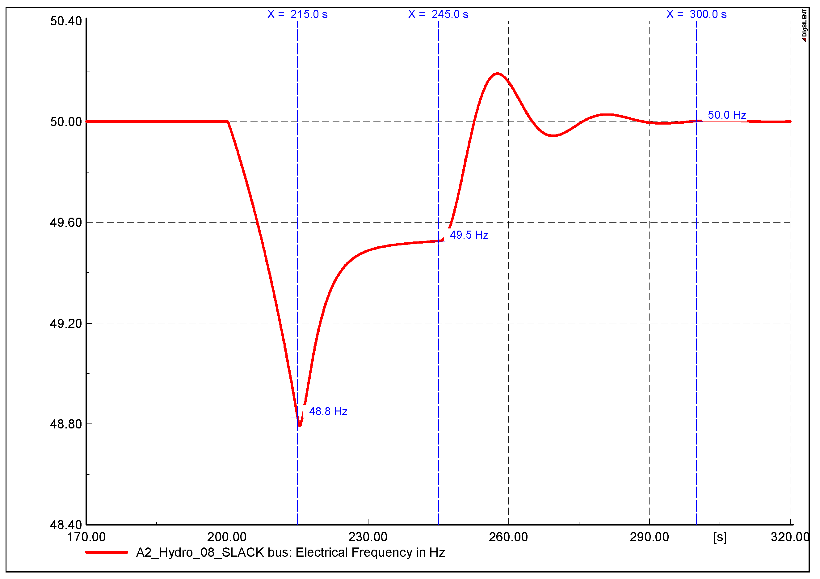
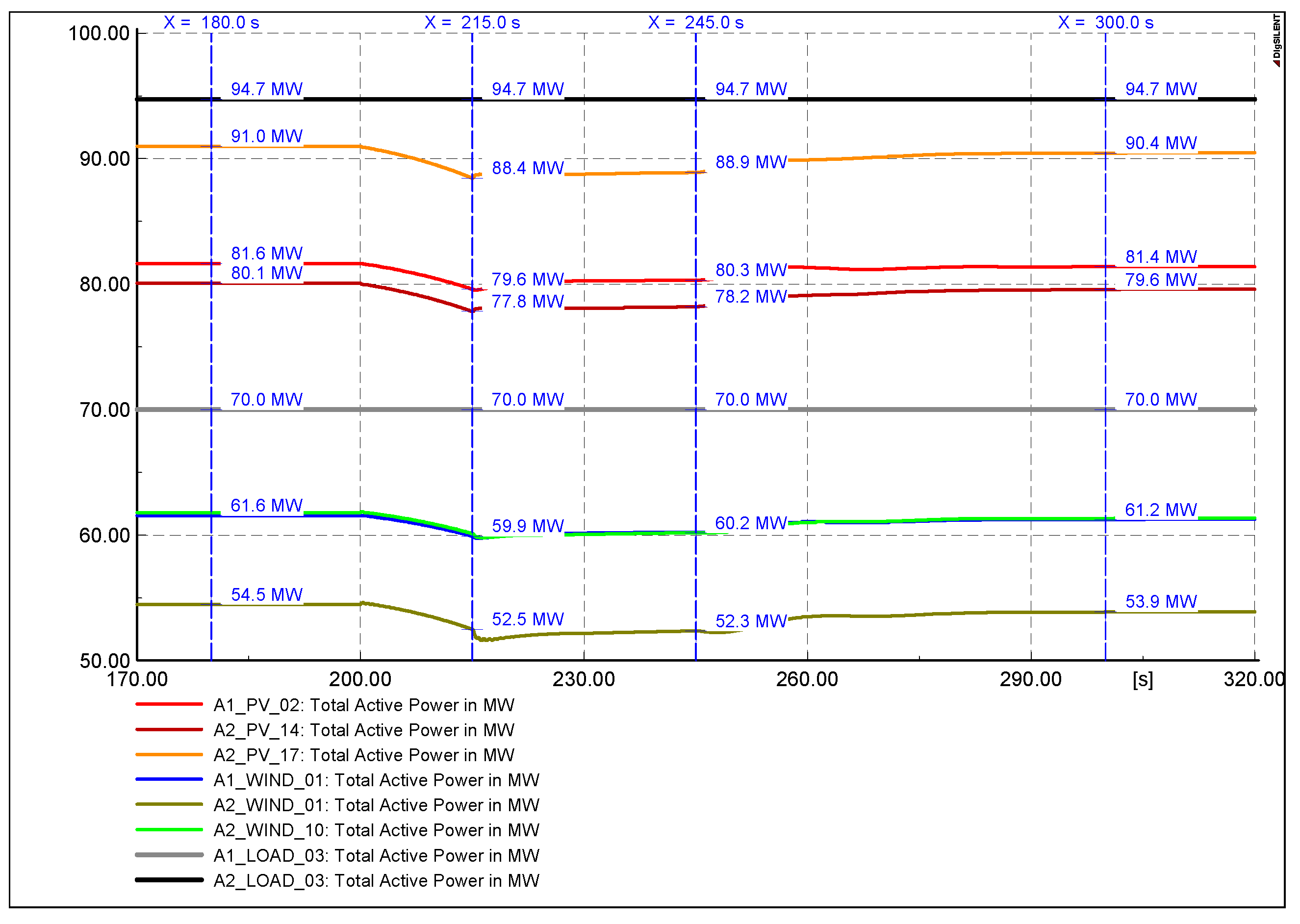
3.3.1. Scenario 1: Reduction in Generating Capacity of Solar Power Plants in Area 1

Scenario 1 assumes that some solar power plants in Area 1 have reduced generating capacity due to cloud cover. The amount of capacity decreased is about 90 MW (about 5% of the total generating capacity of solar power plants in Area 1). This event is simulated to occur at t = 200 s. Figure 8 presents the oscillation process of the system frequency in Scenario 1. Here, the frequency gradually decreases from 50 Hz to 48.8 Hz due to the inertia of the power system and the instantaneous impact from the entire governor system of all the generators. After a period of 15 s following the system frequency change (t = 215 s), the generators responsible for adjusting the primary frequency will bring the frequency from 48.8 to 49.5 Hz within 15 s and maintain that frequency for 30 s to prepare the secondary control. After a period of 45 s following the system frequency change (t = 245 s), the AGC system sends $d{p}_i^g$ signals to these generators and begins to increase the power to bring the frequency from 49.5 Hz to 50 Hz. The frequency oscillates and stabilizes after t = 300 s.

Figure 9 shows the operations of the hydroelectric power units in Area 1 that are assigned to undertake the primary and secondary frequency controls. At t = 200 s, all generators in the system respond to the sudden change in frequency according to their 5% slope characteristic. The system frequency is suppressed and does not decrease rapidly. At t = 215 s, the generators shown in Figure 9 increase their power to perform the primary frequency control. The initial signals of the PI controller in the AGC system cause the power of the primary frequency generators to surge, then gradually decrease to the required amount of power for the primary control within 30 s. At t = 245 s, the AGC system operates to bring the frequency to the rated value. The generators shown in Figure 9 are required to increase their power to bring the frequency from 49.5 to 50 Hz. The $d{p}_i^g$ signals are sent to generators A1_hydro_01(04,05,06,07), causing their power to increase. The frequency recovers, surpasses 50 Hz, and oscillates between t = 250 s and t = 300 s. After t = 300 s, these generators establish a new power output to compensate for the 90 MW of solar power decrease in the system. The generating capacity increases compared to the original to compensate for the reduced power of the RES. The total increased generating capacity is 90 MW (reduced capacity of RES) and divided according to the ${\lambda }_i^g$ of each generator in Figure 9.

Figure 10 shows the operation of the generators equipped with a governor in Area 1 and these are not required to participate in the frequency control. They only support the primary frequency control process in the first 15 s. At t = 200 s, when a decrease in solar power capacity occurs on the system, all generators equipped with governors will react immediately according to their slope characteristics. In Figure 10, from t = 200 s to t = 215 s, we see that the generators increase their power to limit the decrease in frequency on the system. At t = 215 s, they reduce the corresponding amount of power to give the primary frequency power to generator A1_Hydro_01(04,05,06,07). Then, their governor operates according to the measured frequency signal $f_{meas}$ and returns the output power to its original value within 30 s. At t = 245 s, the governor reacts according to the slope characteristic. When the frequency increases, the output power decreases and vice versa. Their oscillation synchronizes with the power system frequency and returns to its original capacity after t = 300 s. In short, after the frequency control loops, these generators maintain the same amount of power as they had originally.

There is a difference between the total power of the generators shown in Figure 9 at t = 245 s and that at t = 300 s. The total output power of the generators in the primary control stage is greater than that at the secondary control stage. The reason is that, when the power system frequency decreases, the converter system of solar and wind power plants reacts according to its droop characteristic. This is presented in Figure 11. When the frequency decreases, starting from t = 200 s, the output power of the renewable energy power plant decreases and then increases back to near the original value when the frequency has returned to 50 Hz (after t = 300 s). Therefore, the total output power of the primary control stage is larger than the secondary control stage by an amount that is the reduced capacity of the remaining RESs on the grid. In Figure 9, the total increased generator capacity at t = 300 s is greater than 90 MW (specifically 112.7 MW) because the RESs have not fully recovered to their original generating capacity. In addition, the study also assumes that the load in the simulation is constant. Two typical loads, A1_Load_01 and A2_Load_02, are shown in Figure 11.

The operation of generators in Area 2 and power exchange on tie-lines are shown in Figure 12. In particular, generator A2_Thermal_01 only contributes to the first stage of the frequency control process using the slope characteristic. Generators A2_Hydro_01 and A2_Hydro_02 play a key role in controlling the primary and secondary frequencies when an event occurs in Area 2. In this scenario, their primary stage is to prevent the frequency from dropping too rapidly. From t = 200 s to t = 215 s, their governors respond by swiftly increasing their output power. The system’s power decrease occurs in Area 1, so the two hydroelectric generators in Area 2 do not participate in increasing the capacity to return the frequency to the rated value. The generators in Area 2 all maintain their original capacity at the end of the control process. In addition, Figure 12 also shows the transmission power on two tie-lines. The negative value here only shows the direction of the power flow. The power flow is transferred from Area 1 to Area 2, with a total capacity of about 129 MW. After the event of solar power decrease mentioned above, the transmission capacity remained almost unchanged. There is no requirement for assistance from Area 2 because Area 1 has a significant amount of reserve capacity. This complies with the principle of ensuring $\Delta P_{ij}=0$, giving priority to frequency adjustment by generators in the area where the event occurs.

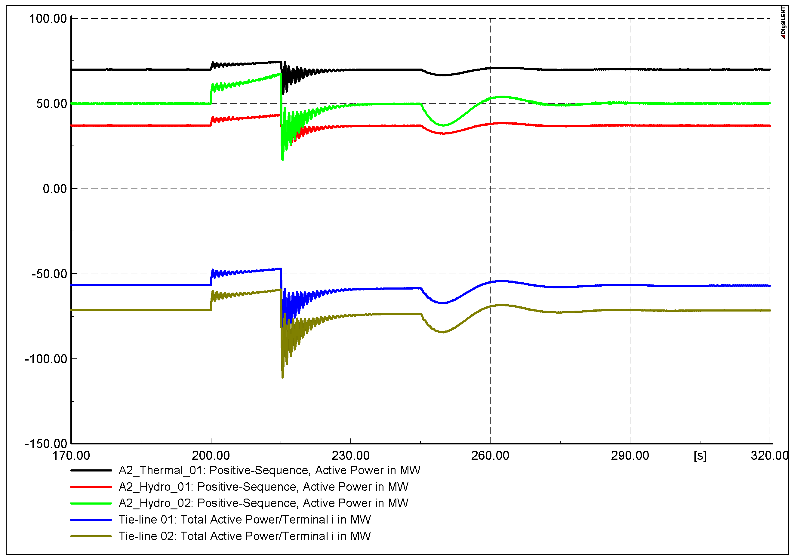
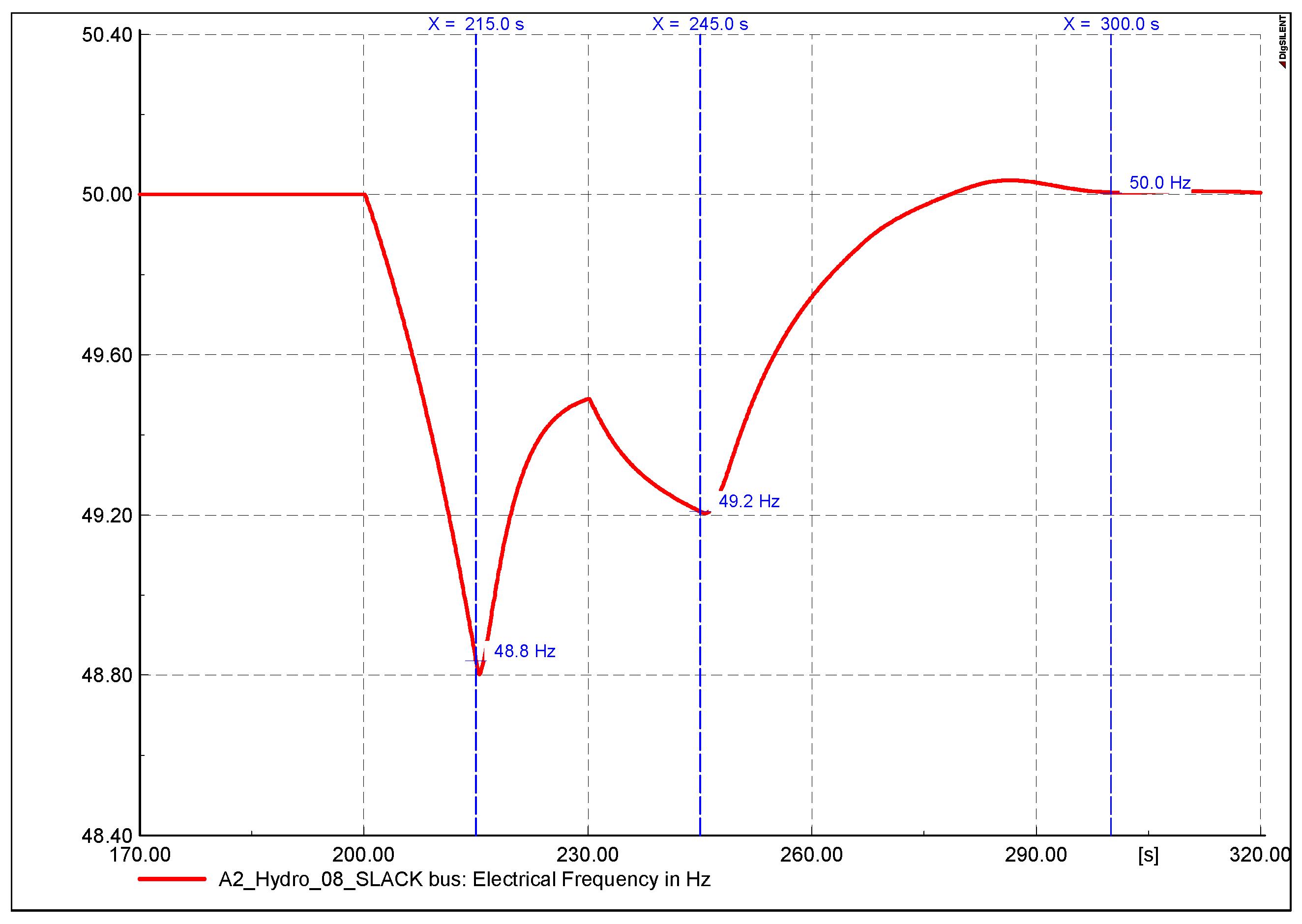
3.3.2. Scenario 2: Reduced Power-Generation Capacity of Solar Power Plants and Frequency-Controlled Generator in Area 1—Forcing Shutdown due to Problems

Similar to Scenario 1, Scenario 2 assumes that some solar power plants in Area 1 reduce their generating capacity due to cloud cover at t = 200 s. The amount of capacity decreased is about 90 MW (about 5% of the total generating capacity of solar power plants in Area 1). Then, during the frequency adjustment process, generator A1_Hydro_07 encountered a problem at t = 230 s and had to shut down. This is the time when the system is in the primary frequency control loop. Figure 13 presents the oscillation process of the power system frequency in Scenario 2. The processes are similar to those analyzed in Scenario 1. At t = 230 s, the system frequency begins to decline from 49.5 Hz down to 49.3 Hz. At t = 245 s, the secondary frequency control loop starts working and the system frequency is increased. Unlike Scenario 1, due to the loss of a frequency-controlled generator in Area 1, the power system frequency in Scenario 2 increases more slowly and stably. In Scenario 1, the frequency exceeds the nominal value and oscillates, starting at t = 250 s and stabilizing at t = 300 s. In Scenario 2, the frequency gradually increases to the nominal value at t = 275 s, then fluctuates slightly and stabilizes at t = 300 s.

Figure 14 illustrates the working process of generators participating in the AGC system in Area 1, while Figure 15 shows the process for non-participating generators in the same area. During the period from t = 200 s to t = 230 s, their operation process is similar to the analysis in Scenario 1. At t = 230 s, generator A1_Hydro_07 has a problem; thus, it is forced to shut down. Immediately, the governors equipped with the generators responded to the decrease in frequency due to the loss of generator A1_Hydro_07. In Figure 15, the generators that do not participate in the AGC increase their power instantaneously according to the droop characteristic, so there is a sharp peak in the power of these generators at t = 230 s. The power increase does not continue as it did during the reaction from t = 200 s to t = 215 s because of the impact of the generators participating in the AGC. In Figure 14, at t = 230 s, generator A1_Hydro_01(04,05,06) does not have a power spike like the generators shown in Figure 15. They increase power gradually from t = 230 s to t = 245 s because they are in the primary frequency control loop. Therefore, there is a difference in response between the generators shown in Figure 14 and Figure 15 after the A1_Hydro_07 generator loss event. At t = 245 s, the secondary frequency control process begins; generator A1_Hydro_01(04,05,06) receives signals from the AGC system to increase output power, bringing the system frequency to the nominal value. Generators A1_Hydro_04(05,06) increase their power, then gradually decrease; this is similar to what happens in Scenario 1. More specifically, because the participation coefficient is the largest among generators participating in the AGC, A1_Hydro_01 increases to maximum power and maintains that power for about 20 s. The idea of maintaining this maximum power is to maintain the increase in the system frequency and compensate for the decline in power of the remaining RESs (shown in Figure 16). The generators participating in the AGC establish new output power after the events, after t = 320 s.

Figure 16 shows the power characteristics of the load and the remaining RESs on the system in Scenario 2. It can be seen that the RES output powers respond to the system frequency. From t = 200 s to t = 245 s, the RESs’ capacities decrease due to a drop in frequency. Starting from t = 245 s, their output power steadily rises as the system frequency begins to recover. The load capacity on the system is assumed to be constant similar to Scenario 1.In addition, Figure 17 presents the response of the generators in Area 2 and the power exchanged between the two areas on the tie-lines. The generators in Area 2 do not participate in the frequency-regulation process in Area 1, so they only respond according to frequency through their governor controller. After the events, the output power of these generators remains unchanged, and the power on the 2 tie-lines is also kept constant.

4. Conclusions

In this paper, a model of a two-area AGC control approach is developed and tested on a power system with high RES penetration. As a result, this model worked correctly when there was a sudden drop in the large output of solar power plants. The frequency control loops of the AGC model operate correctly according to the algorithm that brings the $ACE$ signal to zero value. This AGC model also ensures that the mobilization of generators to participate in secondary frequency regulation is only performed in the area where events occur. This ensures that the flow of power exchanged between areas via tie-lines is maintained, avoiding exceeding the transmission limit and causing instability in the system. The power system also ensures stable operation even with continuous capacity changes occurring at the renewable energy plants. In the future, the AGC model in this study needs to be upgraded; some advanced problems in the power system must be solved:

• Control of the power flow on the transmission lines in a given area to ensure that it is not overloaded.
• Experiment with a larger system model that is divided into more areas. In addition to the principle of geographical division, it is necessary to study the scenario of dividing a large area into many small areas according to internal lines that are often overloaded.
• Apply advanced control strategies such as adaptive control, machine-learning-based approaches, and artificial intelligence to the AGC system to make monitoring and control capabilities more flexible.
• Combine the AGC model with models of the electricity market (economic dispatch) and auxiliary services in the power system.

References

1. International Energy Agency (IEA). Renewables 2023; IEA: Paris, France, 2024; p. 141. [Google Scholar]
2. Imperial College Business School; International Energy Agency. ASEAN Renewables: Opportunities and Challenges; International Energy Agency: Paris, France, 2023. [Google Scholar]
3. Deputy Prime Minister of Vietnam. Decision 500/QD-TTg—The Power Development Plan VIII; Prime Minister of Vietnam: Hanoi, Vietnam, 2023. [Google Scholar]
4. Le, L.H.; Le, N.K. A thorough comparison of optimization-based and stochastic methods for determining hosting capacity of low voltage distribution network. Electr. Eng. 2023, 106, 385–406. [Google Scholar]
5. Hieu, N.H.; Lam, L.H. Using double fed induction generator to enhance voltage stability and solving economic issue. In Proceedings of the 2016 IEEE International Conference on Sustainable Energy Technologies (ICSET), Hanoi, Vietnam, 14–16 November 2016; IEEE: Piscataway, NJ, USA, 2016; pp. 374–378. [Google Scholar]
6. Liang, X.; Andalib-Bin-Karim, C. Harmonics and mitigation techniques through advanced control in grid-connected renewable energy sources: A review. IEEE Trans. Ind. Appl. 2018, 54, 3100–3111. [Google Scholar] [CrossRef]
7. Soleimanisardoo, A.; Kazemi-Karegar, H. A Protection Strategy for MV Distribution Networks with Embedded Inverter-based DGs. Adv. Electr. Comput. Eng. 2022, 22. [Google Scholar] [CrossRef]
8. Du, P.; Matevosyan, J. Forecast system inertia condition and its impact to integrate more renewables. IEEE Trans. Smart Grid 2017, 9, 1531–1533. [Google Scholar] [CrossRef]
9. Kundur, P.S.; Malik, O.P. Power System Stability and Control; McGraw-Hill Education: New York, NY, USA, 2022. [Google Scholar]
10. Peddakapu, K.; Mohamed, M.R.; Srinivasarao, P.; Arya, Y.; Leung, P.K.; Kishore, D.J.K. A state-of-the-art review on modern and future developments of AGC/LFC of conventional and renewable energy-based power systems. Renew. Energy Focus 2022, 43, 146–171. [Google Scholar] [CrossRef]
11. Gulzar, M.M.; Iqbal, M.; Shahzad, S.; Muqeet, H.A.; Shahzad, M.; Hussain, M.M. Load frequency control (LFC) strategies in renewable energy-based hybrid power systems: A review. Energies 2022, 15, 3488. [Google Scholar] [CrossRef]
12. Çelik, E.; Öztürk, N.; Arya, Y.; Ocak, C. (1 + PD)-PID cascade controller design for performance betterment of load frequency control in diverse electric power systems. Neural Comput. Appl. 2021, 33, 15433–15456. [Google Scholar] [CrossRef]
13. Ali, G.; Aly, H.; Little, T. Automatic Generation Control of a Multi-Area Hybrid Renewable Energy System Using a Proposed Novel GA-Fuzzy Logic Self-Tuning PID Controller. Energies 2024, 17, 2000. [Google Scholar] [CrossRef]
14. Mansour, S.; Badr, A.O.; Attia, M.A.; Sameh, M.A.; Kotb, H.; Elgamli, E.; Shouran, M. Fuzzy logic controller equilibrium base to enhance AGC system performance with renewable energy disturbances. Energies 2022, 15, 6709. [Google Scholar] [CrossRef]
15. Debnath, M.K.; Agrawal, R.; Tripathy, S.R.; Choudhury, S. Artificial neural network tuned PID controller for LFC investigation including distributed generation. Int. J. Numer. Model. Electron. Netw. Devices Fields 2020, 33, e2740. [Google Scholar] [CrossRef]
16. Abo-Elyousr, F.K.; Abdelaziz, A.Y. A novel modified robust load frequency control for mass-less inertia photovoltaics penetrations via hybrid PSO-Woa Approach. Electr. Power Components Syst. 2019, 47, 1744–1758. [Google Scholar] [CrossRef]
17. Wang, J.; Sun, Y. Load Frequency Active Disturbance Rejection Control Based on Improved Particle Swarm Optimization. Electronics 2024, 13, 1268. [Google Scholar] [CrossRef]
18. Rasolomampionona, D.D.; Połecki, M.; Zagrajek, K.; Wróblewski, W.; Januszewski, M. A Comprehensive Review of Load Frequency Control Technologies. Energies 2024, 17, 2915. [Google Scholar] [CrossRef]
19. Alam, M.S.; Chowdhury, T.A.; Dhar, A.; Al-Ismail, F.S.; Choudhury, M.; Shafiullah, M.; Hossain, M.I.; Hossain, M.A.; Ullah, A.; Rahman, S.M. Solar and wind energy integrated system frequency control: A critical review on recent developments. Energies 2023, 16, 812. [Google Scholar] [CrossRef]
20. Chang-Chien, L.R.; Lin, W.T.; Yin, Y.C. Enhancing frequency response control by DFIGs in the high wind penetrated power systems. IEEE Trans. Power Syst. 2010, 26, 710–718. [Google Scholar]
21. Irfan, M.; Iqbal, J.; Iqbal, A.; Iqbal, Z.; Riaz, R.A.; Mehmood, A. Opportunities and challenges in control of smart grids–Pakistani perspective. Renew. Sustain. Energy Rev. 2017, 71, 652–674. [Google Scholar] [CrossRef]
22. Ray, P.K.; Mohanty, A. A robust firefly–swarm hybrid optimization for frequency control in wind/PV/FC based microgrid. Appl. Soft Comput. 2019, 85, 105823. [Google Scholar] [CrossRef]
23. Alqahtani, S.; Shaher, A.; Garada, A.; Cipcigan, L. Impact of the high penetration of renewable energy sources on the frequency stability of the Saudi grid. Electronics 2023, 12, 1470. [Google Scholar] [CrossRef]
24. Gonzalez-Longatt, F.M.; Rueda, J.L. PowerFactory Applications for Power System Analysis; Springer: Berlin/Heidelberg, Germany, 2014. [Google Scholar]
25. Machowski, J.; Lubosny, Z.; Bialek, J.W.; Bumby, J.R. Power System Dynamics: Stability and Control; John Wiley & Sons: Hoboken, NJ, USA, 2008. [Google Scholar]
26. The Ministry of Industry and Trade. Circular No. 25/2016/TT-BCT Regulation on Electricity Transmission System; Petrovietnam Power Corporation: Hanoi, Vietnam, 2016. [Google Scholar]
27. Neplan AG. Turbine–Governor Models, Standard Dynamic Turbine–Governor Systems in NEPLAN Power System Analysis Tool; Technical Report; Neplan AG: Küsnacht, Switzerland, 2013. [Google Scholar]
Figure 1. The droop characteristics of governor.
Electronics 13 02907 g001
Figure 2. The transfer function of the turbine–governor controller.
Electronics 13 02907 g002
Figure 3. The transfer function of the AGC system.
Electronics 13 02907 g003
Figure 4. The composite model of the AGC system.
Electronics 13 02907 g004
Figure 5. The here-presented 106-bus system with a high concentration of RESs.
Electronics 13 02907 g005
Figure 6. The governor controller model is configured in DIgSILENT PowerFactory.
Electronics 13 02907 g006
Figure 7. The governor controller model is configured in DIgSILENT PowerFactory.
Electronics 13 02907 g007
Figure 8. The system frequency oscillation.
Electronics 13 02907 g008
Figure 9. Output power of generators that are responsible for the primary and secondary frequency control in Area 1.
Electronics 13 02907 g009
Figure 10. Output power of generators that do not participate in frequency control in Area 1.
Electronics 13 02907 g010
Figure 11. Output power of renewable energy power plant and typical load in Areas 1 and 2.
Electronics 13 02907 g011
Figure 12. Output power of generators in Area 2 and power exchange on the tie-lines.
Electronics 13 02907 g012
Figure 13. The system frequency oscillation.
Electronics 13 02907 g013
Figure 14. Output power of generators that is responsible for the primary and secondary frequency control in Area 1.
Electronics 13 02907 g014
Figure 15. Output power of generators do not participate in frequency control in Area 1.
Electronics 13 02907 g015
Figure 16. Output power of renewable energy power plant and typical load in Areas 1 and 2.
Electronics 13 02907 g016
Figure 17. Output power of generators in Area 2 and power exchange on the tie-lines.
Electronics 13 02907 g017