LBCNIN: Local Binary Convolution Network with Intra-Class Normalization for Texture Recognition with Applications in Tactile Internet

Abstract

Texture recognition is a pivotal task in computer vision, crucial for applications in material sciences, medicine, and agriculture. Leveraging advancements in Deep Neural Networks (DNNs), researchers seek robust methods to discern intricate patterns in images. In the context of the burgeoning Tactile Internet (TI), efficient texture recognition algorithms are essential for real-time applications. This paper introduces a method named Local Binary Convolution Network with Intra-class Normalization (LBCNIN) for texture recognition. Incorporating features from the last layer of the backbone, LBCNIN employs a non-trainable Local Binary Convolution (LBC) layer, inspired by Local Binary Patterns (LBP), without fine-tuning the backbone. The encoded feature vector is fed into a linear Support Vector Machine (SVM) for classification, serving as the only trainable component. In the context of TI, the availability of images from multiple views, such as in 3D object semantic segmentation, allows for more data per object. Consequently, LBCNIN processes batches where each batch contains images from the same material class, with batch normalization employed as an intra-class normalization method, aiming to produce better results than single images. Comprehensive evaluations across texture benchmarks demonstrate LBCNIN’s ability to achieve very good results under different resource constraints, attributed to the variability in backbone architectures.

1. Introduction

Recognizing and understanding textures is essential in image analysis. This process involves identifying and making sense of detailed patterns that are key to distinguishing different items in pictures. Effective texture recognition is crucial because it enhances a computer’s ability to notice fine details and deeply understand images, leading to more accurate results when recognizing and classifying various materials or objects based on their textures. The ability to accurately capture these textural nuances is what enables more sophisticated image processing techniques, which are increasingly important in a world where visual data is abundant and varied. Additionally, for decades, texture has been essential in image recognition across various domains such as medicine [1], face analysis [2], material sciences [3], object recognition [4], agriculture [5], and terrain recognition [6]. This importance extends to computer vision, particularly in the emerging field of TI, where texture recognition plays a crucial role in enhancing real-time interactive systems. Although there is no universally accepted definition, texture in digital images can be described by local pixel intensity variations, forming spatial patterns that are somewhat independent across different scales [7]. Traditional Convolutional Neural Networks (CNNs) perform well on general images but struggle with the intricate details of texture due to their sensitivity to rigid transformations. Additionally, CNNs with Fully Connected (FC) layers are not well-suited for texture analysis [8]. The spatial correlation in convolutional feature maps, even after passing through FC layers, poses a challenge for standard CNNs in maintaining texture invariance to transformations like translation, rotation, and scaling. To overcome these issues, recent advancements in DNNs have significantly improved texture analysis by utilizing pre-trained models on extensive datasets through transfer learning [9,10,11,12,13]. These methods offer computational efficiency during inference, but retraining the backbone remains computationally demanding. To aggregate features, some methods have employed Global Average Pooling (GAP), which creates robust descriptions resistant to spatial transformations [11,14,15]. Other techniques focus on mid-level features from earlier layers, capturing general image characteristics not specific to particular applications [16]. However, these methods require extensive texture datasets for end-to-end training with deep CNN architectures. A promising new approach involves Local Binary Convolutional Networks (LBCNNs) [17], inspired by traditional LBP [18] intended for texture classification. As demonstrated in [17], LBCNNs offer a substantial reduction in training complexity, presenting a promising and efficient alternative to Local Binary Patterns (LBP) for texture recognition in neural networks. This suitability arises because LBCNNs, leveraging the principles of LBP, are adept at capturing and encoding the local textural patterns within an image, which are crucial for distinguishing between different textures in recognition tasks.

The motivation behind this work stems from the evolving field of Tactile Internet (TI), which aims to enable real-time transmission of touch and haptic information over the internet. One critical component of TI can be texture recognition, which allows systems to understand and interpret the surface quality of objects, encompassing attributes like roughness, smoothness, and patterns. Accurate texture recognition enhances the ability of TI systems to simulate tactile sensations and provide realistic haptic feedback, thereby improving user experience in applications such as virtual reality, robotics, and assistive technologies. In addition to enhancing user experience, texture recognition plays a pivotal role in determining the material type of objects. Different materials often exhibit distinct textural properties, and identifying the texture of a surface can help distinguish whether it is made of wood, metal, or plastic. By leveraging deep neural networks like LBCNIN for texture recognition, systems can achieve both the identification of textures and the inference of material types based on textural features. This dual capability is essential for various scene understanding applications within TI, where accurate tactile perception is crucial. In robotics, for instance, texture recognition enhances object manipulation and handling by providing detailed information about the object’s surface and material properties. Moreover, integrating texture recognition with 3D point cloud semantic segmentation enhances the system’s ability to create detailed reconstructions of physical objects, which is beneficial for tasks requiring precise physical interactions. Semantic segmentation is responsible for identifying and classifying objects, whereas texture recognition may provide more detailed insights into the material composition of these objects, assuming that the surface features and material composition are consistent. It should be noted that in 3D semantic segmentation, the availability of multiview data for objects is beneficial, as it leads to more accurate texture recognition. Instead of direct analysis of a 3D point cloud, multiple 2D images are utilized, each captured from different views. Consequently, the proposed LBCNIN architecture is designed to process batches of data, where each batch is composed of images that belong to the same texture class, depicting the same object. This approach enhances the model’s ability to learn and distinguish between different textures, leading to improved performance in recognizing material types. By using texture information, the system can estimate the volume and mass of objects, providing critical data for applications requiring precise physical interactions. Furthermore, the combination of visual and tactile data enables a more comprehensive understanding of the environment, allowing for advanced material texture simulation and more realistic haptic feedback in VR applications. Employing the LBCNIN architecture, therefore, allows systems to achieve higher accuracy and efficiency in texture recognition, ultimately enhancing performance across a wide range of TI applications.

The main contributions of the presented work are as follows:

• Introducing a novel architecture (LBCNIN) specifically tailored for texture recognition tasks in TI for multi-view images of the same object. This architecture encodes features from the backbone without requiring fine-tuning, utilizing a non-trainable local binary convolution layer inspired by LBP.
• Demonstrating the performance of LBCNIN across various texture benchmarks in comparison with state-of-the-art methods. The evaluation assumes the use of intra-class normalization technique. Additionally, an ablation study on different components of the architecture (BatchNorm2d, Activation functions, LBC layer, and GAP) highlights their respective impacts on accuracy, providing insights into the architecture’s effectiveness.
• Conducting an extensive evaluation of different backbone architectures within the context of texture recognition tasks, the study assessed the performance of various backbones such as MobileNet V2 1.4, ResNet18, ResNet50, and ConvNeXt-XL, across diverse texture datasets. The evaluation encompassed an ablation study on different components of the proposed architecture and exploring the effectiveness of different activation functions in the proposed feature encoding scheme. Moreover, 2D t-SNE and GradCAM visualizations provided insights into the model’s behavior, while confusion cases highlighted its limitations. CPU and GPU computation times for different backbone architectures were also compared.

With the assumption that intra-class normalization is performed within a batch of samples from the same class, the proposed architecture achieved the best results in the presented comparison on datasets such as DTD and KTH-2b. Using the lightweight MobileNet V2 1.4 backbone, it surpassed all methods utilizing more computationally intensive backbones like ResNet18 and ResNet50 for these datasets. However, for the other two tested datasets, GTOS and GTOS-Mobile, the achieved accuracy with ResNet18 and ResNet50 was lower compared to other methods. Notably, the proposed architecture achieved the best results with the ConvNeXt-XL backbone pre-trained on the ImageNet-21K dataset, which demands more computational resources. The ability of the proposed algorithm to attain high accuracy with small datasets and using a backbone with low computational demands makes it particularly suitable for applications in texture recognition, where available training data may be limited and devices may have constrained computational capabilities.

The rest of this paper is structured as follows: Section 2 provides an overview of related works in the field of texture recognition. Section 3 details the proposed architecture and its implementation. In Section 4, the datasets used, the experimental protocols, comparisons with state-of-the-art methods, an ablation study on different architectural components, and investigations into specific activation functions used in the LBCNIN encoding phase are presented. This section also includes an evaluation of the stability of LBCNIN accuracy with various random masks of LBC, as well as representations of confusion matrices, 2D t-SNE features, GradCAM visualizations, and some incorrectly classified samples. At the end of this section, timing performance and limitations of the presented work are provided. Finally, Section 5 concludes the paper, summarizing key findings and contributions.

2. Related Work

Traditional methods for texture analysis and recognition usually involved a systematic approach highly dependent on the selected model for image representation. These methods relied on hand-crafted features intended to be invariant to scale, illumination, and translation. For instance, Lowe et al. [19] introduced the Scale Invariant Feature Transform (SIFT), which operates by identifying local minimums and maximums within a scale pyramid. Lazebnik et al. [20] present the Rotation Invariant Feature Transform (RIFT), which achieves rotation invariance by utilizing histograms of relative gradient orientation within rings. Two other methods, namely Histogram of textons (e.g., [21]) and Bag-of-Visual-Words (BoVW) of texture (e.g., [20]), involve crucial steps of local patch encoding and global feature aggregation. The Fisher Vector (FV) [20] introduces second-order statistics for encoding, providing an alternative approach. Another method known as Vector of Locally Aggregated Descriptor (VLAD) [22] aggregates first-order statistics by accumulating differences between a local descriptor and its corresponding matches. Another simple yet powerful handcrafted descriptor is LBP [18]. It achieves grayscale invariance by sequentially thresholding the intensity of neighboring elements to that of the central element within the patch. Maximal circular bit-shift codes are utilized to achieve rotational invariance.

More recently, there’s been a growing use of CNNs as powerful tools for extracting texture features, following their success in computer vision. This mirrors the overall trend towards deep learning in texture analysis. One of the earliest breakthroughs in this field can be credited to Bruna et al. [23]. The authors utilized convolutional layers to implement scattering transformation for texture classification. Despite the benefits of the scattering transform’s invariance to specific deformations, their CNN utilizes predetermined weights (basic wavelet filters), limiting its ability to harness the full potential of Deep Learning (DL). Introducing a learnable approach, Cimpoi et al. [24] compared two models for feature extraction. The first utilized a CNN architecture with FC layers, while the second applied a FV as a pooling method on a pre-trained CNN. They found that the CNN with FC layers was ineffective for texture classification, as its output was highly correlated with the spatial order of pixels. In other research, Fujieda [15] and Andrearczyk et al. [14] enhanced robustness by using a GAP layer. However, GAP can discard important details as it simply averages the feature map of each channel. To overcome this limitation, Lin and Maji [25] proposed bilinear pooling to better capture the relationships between channels. Several studies have proposed end-to-end models that allow for fine-tuning the backbone specifically for texture classification. Zhang et al. [26] introduced a Deep Texture Encoding Network (DeepTEN), which integrates dictionary learning and feature pooling within a CNN architecture. This approach learns an unordered representation, yielding strong performance in material classification. However, since textures and materials do not always lack order, incorporating local spatial information remains crucial. Xue et al. [27] presented a Deep Encoding Pooling Network (DEPNet), which merges features from the texture encoding layer of DeepTEN with GAP to capture both local spatial information and global context in images. Bu et al. [28] proposed a locality-aware coding layer for texture classification within an end-to-end framework (LSCNet). This method uses convolutional layer activations and complex optimization to enforce locality and sparsity, capturing class-specific information and generating robust features. Zhai et al. [11] introduced a method for learning visual attributes in texture recognition. Their model, MAPNet, utilizes a multi-branch architecture to iteratively learn texture attributes. Feature aggregation is performed using spatially-adaptive GAP on each branch. In their subsequent work [10], they proposed DSRNet, which incorporates a dependency learning module to capture spatial relationships among texture primitives and extract structural information. Peeples et al. [29] proposed HistRes, a texture classification network integrating traditional histogram features into deep learning. Replacing the GAP layer, HistRes enhances accuracy by directly extracting histogram information from the final feature map. Chen et al. [12] proposed Cross-Layer Aggregation of a Statistical Self-similarity Network (CLASSNet). This CNN module integrates a distinctive feature aggregation method using a differential box-counting pooling layer to describe the statistical self-similarity present in texture images. Xu et al. [30] introduced FENet, which utilizes hierarchical fractal analysis to capture the fractal properties of spatial arrangements present in CNN feature maps. Mao et al. [31] employed deep Residual Pooling Network (RPNet) for texture recognition. It merges a residual encoding module, which retains spatial details, with an aggregation module that produces orderless features. Song et al. [32] presented a Multi-Scale Boosting Feature Encoding Network (MSBFEN) for texture recognition. MSBFEN uses a prior-guided feature extraction method to extract multi-scale features with texture priors, followed by a multiscale texture encoding technique. A multi-scale boosting learning method is then applied to recognize the texture. Recently, Chen et al. [33] introduced a Deep Tracing Pattern encoding Network (DTPNet), which processes feature maps from multiple backbone layers. It encodes local patches with binary codes and aggregates them into a histogram-based global feature. Zhai et al. [34] proposed Multiple Primitives and Attributes Perception (MPAP) network. MPAP extracts features by integrating bottom-up structure and top-down attribute relations within a unified multi-branch framework. Scabini et al. [35] proposed a new method for texture recognition named Random encoding of Aggregated Deep Activation Maps (RADAM). The method involves encoding the output at various depths of a pre-trained backbone with a Randomized Autoencoder (RAE). The RAE is locally trained for each image and its decoder weights form a feature representation fed into a linear SVM, eliminating the need for backbone fine-tuning.

Despite incorporating certain elements and ideas from the previously mentioned approaches, such as the utilization of a pre-trained backbone without fine-tuning, the proposed LBCNIN method significantly diverges in its approach to encode the final texture representation. While some of the aforementioned methods employ end-to-end training, LBCNIN shares similarities with the RADAM method. However, unlike RADAM, LBCNIN does not utilize an autoencoder. Instead, it employs a simple LBC layer to encode the feature maps from the backbone’s final layer and intra-class normalization technique true batch normalization. The inspiration for the LBC layer originates from the research outlined in [17]. This approach provides an alternative to the convolutional layers commonly found in standard CNN architectures.

3. Proposed Method

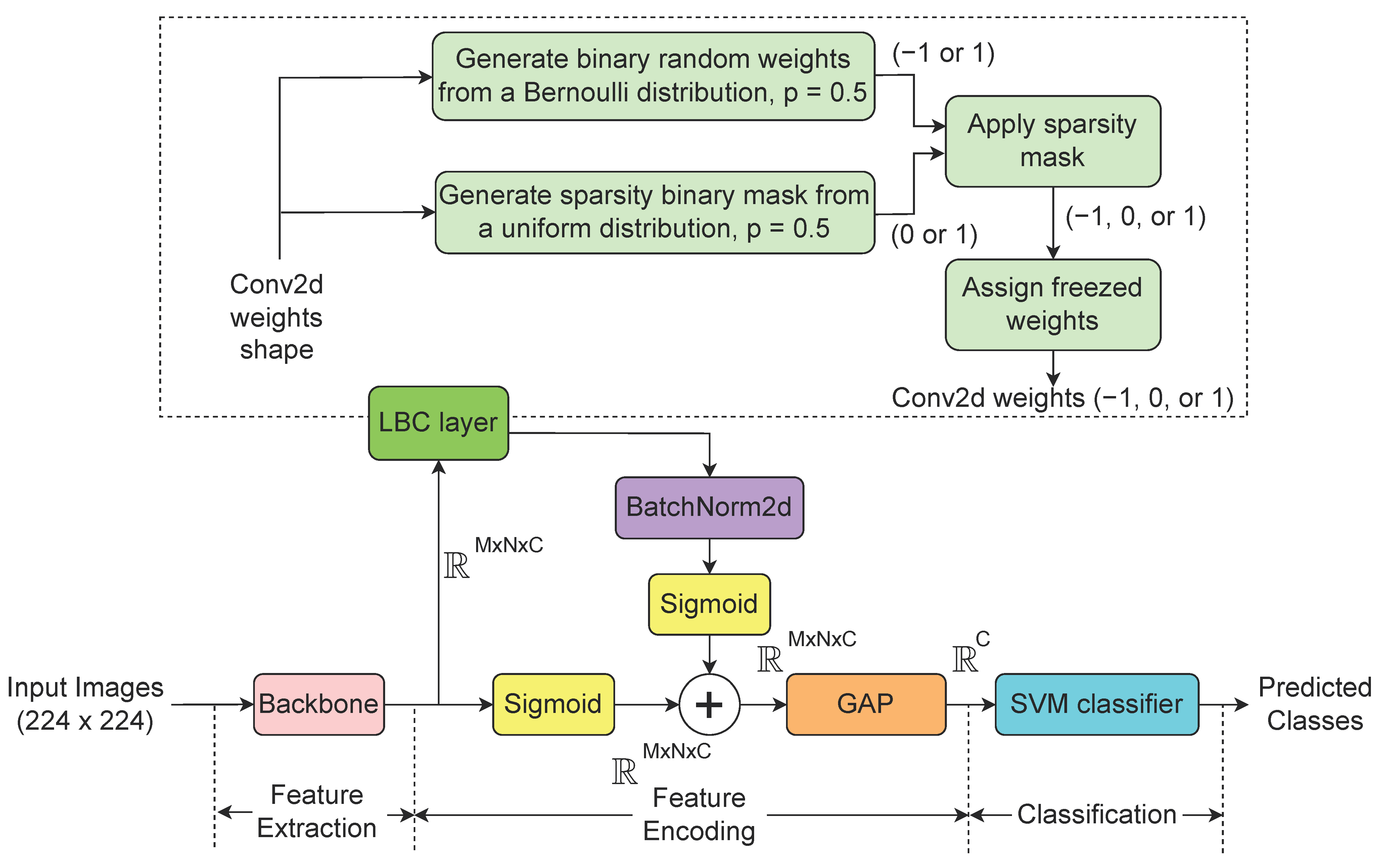
3.1. LBCNIN Architecture

The proposed LBCNIN architecture for classifying texture images is illustrated in Figure 1. It operates in three distinct phases: Feature Extraction, Feature Encoding, and Classification.

This standard structured approach ensures a systematic handling of texture recognition tasks, starting with the extraction of essential image features using a pre-trained backbone. Fine-tuning the backbone is avoided due to the limited dataset, which could lead to overfitting and requires significant computational resources. Feature Encoding is essential to enhance the representation of texture features, leveraging techniques like LBC to refine and extract discriminative information. Finally, the classifier employs SVM rather than FC layers due to the effectiveness of SVM in handling high-dimensional data. Here are detailed descriptions of each step:

Feature Extraction: This phase involves extracting high-level features from the input image. Motivated by the need for varying trade-offs between computational efficiency and effectiveness, the LBCNIN architecture has been investigated with different backbones: MobileNet V2 1.4 [36] (1.4 channel multiplier), ResNets [37] (18 or 50), and ConvNeXt-XL [38] pre-trained on ImageNet-21K. These pre-trained networks have been shown effective in capturing essential patterns and representations from images.

Let $\mathbf{x}\in {\mathbb{R}}^{M\times N\times C}$ denote the feature tensor outputted by the backbone, where $M\times N$ is the spatial resolution, and C is the number of tensor’s channels. To ensure higher spatial resolution, which is critical for capturing detailed texture information, the spatial downsampling rate of the backbone network was adjusted, resulting in a consistent resolution $(M\times N)$ of $28\times 28$ for all backbones. However, the number of channels C of each backbone’s feature tensor differs, reflecting their varying capacities to capture and represent features. Specifically:

• MobileNet V2 1.4: $\mathbf{x}\in {\mathbb{R}}^{28\times 28\times 448}$,
• ResNet18: $\mathbf{x}\in {\mathbb{R}}^{28\times 28\times 512}$,
• ResNet50 and ConvNeXt-XL on ImageNet-21K: $\mathbf{x}\in {\mathbb{R}}^{28\times 28\times 2048}$.

Feature Encoding: In this phase of the LBCNIN architecture, the incorporation of a LBC layer stands out as a key innovation. Drawing inspiration from the effectiveness of LBP in texture classification, this phase leverages the distinct characteristics of the LBC layer outlined in [17]. The LBC layer in [17] consists of fixed sparse pre-defined binary convolutional filters that are not updated during the training process, a non-linear activation function, and a set of learnable linear weights 1 × 1. However, in LBCNIN encoding, the last 1 × 1 convolutional layer is avoided to exclude the trainable part, simplify the model and further reduce the number of parameters.

The intuition behind using the LBC layer is rooted in its design principles, which are motivated by LBP. LBP is a robust hand-crafted descriptor that extracts local texture information by comparing the intensity of neighboring pixels to a central pixel within an image patch, generating a binary string that encodes these texture patterns. Similarly, the LBC layer employs binary convolutional filters to effectively capture local texture features. This method provides substantial parameter savings compared to standard convolutional layers, leading to smaller model sizes and lower computational costs. By capitalizing on the sparse and binary characteristics of these filters, the LBC layer closely approximates the performance of standard convolutional layers while maintaining computational efficiency. This innovation significantly enhances the LBCNIN architecture’s ability to achieve high accuracy in texture classification tasks, as evidenced by empirical results.

The process can be detailed as follows:

• Sigmoid Activation: The feature tensor $\mathbf{x}$ undergo normalization and introduction of non-linearity through a Sigmoid function, ensuring all features are scaled between 0 and 1, which stabilizes the feature values for subsequent processing:

  $$\sigma \left(\mathbf{x}\right)={\displaystyle \frac{1}{1+exp(-\mathbf{x})}}.$$

  (1)
• LBC Layer [17]: The LBC layer introduces sparsity by generating binary random weights ${\mathbf{W}}_b$ ($-1$ or 1) through a Bernoulli distribution with a probability of 0.5. Additionally, a binary mask $\mathbf{M}$ (0 or 1) is created from a uniform distribution. The binary mask is applied element-wise to the weights, resulting in final weight values of $-1$, 0, or 1:

  $${\mathbf{W}}_L={\mathbf{W}}_b\circ \mathbf{M},$$

  (2)

  where ∘ denotes element-wise multiplication (the efficacy of the LBC layer is further demonstrated through the ablation study presented in Section 4.3). The sparse weights are then used in a 2D convolution operation on the features extracted by the backbone network:

  $$\mathbf{y}=\mathbf{x}\ast {\mathbf{W}}_L,$$

  (3)

  where ∗ denotes the convolution operation. This step mimics the effect of learnable parameters while keeping the layer non-trainable, reducing computational complexity and retaining essential texture patterns. In the convolution operation a kernel size of 3 × 3 is selected for its computational efficiency. Further testing indicates that an increase in kernel size does not yield an improvement in performance.
• Batch Normalization: The convolved feature tensor is normalized using BatchNorm2d, which standardizes the data and ensures consistent feature distribution among the samples within the same class:

  $${\mathbf{y}}_{\mathrm{norm}}=\mathrm{BatchNorm}2\mathrm{d}\left(\mathbf{y}\right).$$

  (4)
  The use of the BatchNorm2d layer serves also as an intra-class normalization technique, which can significantly improves performance by ensuring that the input to activation functions in neural networks is normalized, thus reducing internal covariate shift [39]. This normalization process is beneficial within batches of images from the same class, as it helps the architecture learn more efficiently. By conducting additional testing, it has been determined that the optimal batch size for the process is 32. This size is also chosen to ensure the stability and consistency of the normalization process during inference.
• Second Sigmoid Activation: A Sigmoid activation is applied to the convolved normalized feature tensor to further refine the features and intensify non-linear transformations:

  $$\sigma \left({\mathbf{y}}_{\mathrm{norm}}\right)={\displaystyle \frac{1}{1+exp(-{\mathbf{y}}_{\mathrm{norm}})}}.$$

  (5)
  The effectiveness of using these activation functions is further emphasized in Section 4.3 and Section 4.4.
• Feature Summation: The initial Sigmoid-transformed features and the processed features are summed, retaining both the original and enhanced information:

  $$\mathbf{z}=\sigma \left(\mathbf{x}\right)+\sigma \left({\mathbf{y}}_{\mathrm{norm}}\right).$$

  (6)
  This combination leads to a more comprehensive feature representation.
• GAP: Finally, a GAP layer is employed to reduce the dimensionality of the combined features. GAP summarizes each encoded feature tensor into a single value by averaging, effectively capturing the most important texture features while reducing the computational load:

  $${\mathbf{z}}_{\mathrm{GAP}}={\displaystyle \frac{1}{M\times N}}\sum _{i=1}^M\sum _{j=1}^N{\mathbf{z}}_{i,j}.$$

  (7)

This process ensures that the features undergo a distinct encoding procedure, capturing intricate patterns crucial for texture classification tasks.

Classification: This phase is the only learnable part of the LBCNIN architecture. In the classification phase, the encoded features, now represented as a single vector from the GAP layer, are fed into a SVM classifier with linear kernel. SVMs are effective in handling high-dimensional data and finding optimal decision boundaries by maximizing the margin between classes. SVM is also computationally efficient, contrasting with K-Nearest Neighbors (KNN), which can be slower due to its reliance on distance calculations for each test instance. The convex nature of the SVM objective function guarantees a unique and globally optimal solution, providing consistency and reliability in classification results. The decision to use an SVM is further supported by the RADAM study [35], which highlights its superior performance on textured images compared to other classifiers like Linear Discriminant Analysis (LDA). This positions SVM as a robust and efficient choice for the proposed classification architecture.

3.2. Implementation Details

The extraction and encoding part of the algorithm is implemented in PyTorch-GPU (v1.12.1) [40] on a machine equipped with an Intel Xeon E5-2640 v3 CPU operating at 2.60 GHz (8 cores), 32 GB of RAM, and evaluated on an NVIDIA GeForce RTX 2080 Ti GPU. The backbone architectures utilized are sourced from the PyTorch Image Models library (timm) [41]. The batch size is configured to 32, with each input image being RGB and sized at 224 × 224 pixels. The classification part (i.e., SVM) is implemented using the scikit-learn library (v.0.6.7) [42]. It should be noted that the ResNet50 backbone used is sourced from [43] via the timm library due to its better achieved results.

4. Experiments

4.1. Datasets and Experimental Protocols

To evaluate the proposed LBCNIN architecture, four datasets were selected for their diverse representation of textures and materials. The same evaluation protocols are used as in [35] and several other methods. The average accuracy along with standard deviations across the splits (as explained further) are provided as a performance result. Here is a brief description of each dataset along with its evaluation protocol:

• Describable Texture Dataset (DTD) [13]: This dataset consists of 5640 images categorized into 47 distinct texture classes. It is evaluated using the 10 provided splits for training-testing along with the dataset, ensuring robust performance metrics across different subsets. The same evaluation protocol is used in [30,31].
• KTH-TIPS2-b [8] (KTH-2-b): Featuring 4752 images from 11 different material categories, this dataset employs a fixed set of 4 splits for 4-fold cross-validation. This setup allows the model to be trained and tested on diverse subsets, promoting generalized learning. The same splitting scheme is also used in [34].
• Ground Terrain in Outdoor Scenes (GTOS) [44]: This extensive dataset includes 34,105 images representing 40 outdoor ground material classes. It utilizes a fixed set of 5 train/test splits, offering a robust evaluation framework for models designed to classify ground terrain textures. The same evaluation splits are used in [10,11,12,26,30,32,33].
• GTOS-Mobile [27]: Comprising 100,011 images captured via a mobile phone, this dataset features 31 different outdoor ground material categories. It is divided into a single train/test split, reflecting real-world mobile data collection scenarios. The same evaluation protocols are utilized in [10,11,12,32,33].

Before going into comparisons with state-of-the-art methods, in the next subsection, a notable difference is that LBCNIN’s results are achieved by employing batch normalization on batches of images from the same class, unlike all state-of-the-art methods which require a single image for inference. Therefore, the presented comparison may not be entirely equitable. However, the proposed LBCNIN architecture proves to be particularly advantageous for handling the multiview data from 3D semantic segmentation.

4.2. Comparison with State-of-the-Art Methods

The following section discusses the performance of the proposed LBCNIN architecture in comparison with state-of-the-art methods across the four datasets described in Section 4.1. The comparison, as shown in

Table 1. Performance comparison of the proposed architecture LBCNIN in terms of accuracy (%) and standard deviations (±) with state-of-the-art methods. The backbones (along with their number of parameters and GFLOPs) are grouped into row blocks based on their processing capacity. The top results for each dataset in each block are highlighted in bold. The best results, regardless of the used backbones, are underlined. The reference source in square brackets next to each method indicates that the results are taken from the original paper referred to by that source. If a second reference is listed, it signifies that the results are sourced from the subsequent reference.

Method	Backbone	Backbone Params * (Millions)	Backbone GFLOPs *	DTD	KTH-2-b	GTOS	GTOS-Mobile
RADAM light [35]	MobileNet V2 1.4	6	0.77	73.1 ± 0.9	86.8 ± 3.1	81.7 ± 1.7	78.2
LBCNIN (proposed) **				87.2 ± 0.8	90.4 ± 5.0	83.5 ± 1.6	80.6
DeepTEN [26,33]	ResNet18	12	2	-	-	-	76.1
HistRes [29]				-	-	-	79.8 ± 0.8
DEPNet [27]				-	-	-	82.2
FENet [30]				69.6	86.6 ± 0.1	83.1 ± 0.2	85.1 ± 0.4
RPNet [31,33]				71.6 ± 0.7	86.7 ± 2.7	83.3 ± 2.2	76.6 ± 1.5
MAPNet [11]				69.5 ± 0.8	80.9 ± 1.8	80.3 ± 2.6	83.0 ± 1.6
DSRNet [10]				71.2 ± 0.7	81.8 ± 1.6	81.0 ± 2.1	83.7 ± 1.5
RADAM [35]				68.1 ± 1.0	84.7 ± 3.6	80.6 ± 1.7	79.5
CLASSNet [12]				71.5 ± 0.4	85.4 ± 1.1	84.3 ± 2.2	85.3 ± 1.3
DTPNet [33]				71.8 ± 0.7	86.7 ± 1.3	84.8 ± 2.4	87± 1.2
MPAP [34]				72.4 ± 0.7	87.9 ± 1.5	85.5 ± 1.7	85.5 ± 1.6
LBCNIN (proposed) **				89.3 ± 0.6	89.8 ± 3.7	81.4 ± 1.7	74.7
DeepTEN [26,33]	ResNet50	26	5	69.6	82.0 ± 3.3	84.5 ± 2.9	-
HistRes [29]				72.0 ± 1.2	-	-	-
DEPNet [27]				73.2	-	-	-
FENet [30]				74.2 ± 0.1	88.2 ± 0.2	85.7 ± 0.1	85.2 ± 0.4
RPNet [31,33]				73.0 ± 0.6	87.2 ± 1.8	83.6 ± 2.3	77.9 ± 0.3
MAPNet [11]				76.1 ± 0.6	84.5 ± 1.3	84.7 ± 2.2	86.6 ± 1.5
DSRNet [10]				77.6 ± 0.6	85.9 ± 1.3	85.3 ± 2.0	87.0 ± 1.5
RADAM [35]				75.6 ± 1.1	88.5 ± 3.2	81.8 ± 1.1	81
CLASSNet [12]				74.0 ± 0.5	87.7 ± 1.3	85.6 ± 2.2	85.7 ± 1.4
MSBFEN [32]				77.8 ± 0.5	86.2 ± 1.1	86.4± 1.8	87.6 ± 1.6
DTPNet [33]				73.5 ± 0.4	88.5 ± 1.6	86.1 ± 2.5	88.0 ± 1.2
MPAP [34]				78.0 ± 0.5	89.0 ± 1.0	86.1 ± 1.8	88.1 ± 1.3
LBCNIN (proposed) **				93.5 ± 0.8	91.3 ± 4.7	81.5 ± 2.1	80.8
RADAM [35]	ConvNeXt-XL in ImageNet-21K	350	60.9	83.7 ± 0.9	94.4 ± 3.8	87.2 ± 1.9	90.2
LBCNIN (proposed) **				89.4 ± 0.9	96.1 ± 3.3	87.3 ± 1.6	91.8

* The number of parameters and GFLOPs for the MobileNet V2 1.4 backbone are referenced from [45], for the ResNet (18 and 50) backbones from [46], and for the ConvNeXt-XL in ImageNet-21K from [38]. ** The LBCNIN’s results are achieved by implementing batch normalization within batches of images from the same classes. This approach differs from all state-of-the-art methods and is particularly suited for the multiview data encountered in TI 3D semantic segmentation.

, uses the four backbones described in Section 3.1, with respective number of parameters and GFLOPs noted for each.

For the MobileNet V2 1.4 backbone, which has a relatively low computational demand, the LBCNIN architecture outperforms the RADAM light [35] method, which uses the same pre-trained backbone.

Specifically, LBCNIN achieves a notable improvement in accuracy across all four datasets. For instance, it records 87.2% on the DTD dataset and 90.4% on the KTH-2-b dataset, significantly higher than RADAM light’s 73.1% and 82.6%, respectively. It is noteworthy that the proposed architecture, using this backbone, achieves higher accuracy on the DTD and KTH-2-b datasets compared to all state-of-the-art methods that utilize the significantly more complex and resource-intensive ResNet18 and ResNet50 backbones. Despite achieving the highest average accuracy for the KTH-2-b dataset, a notable deviation across the tested folds of ±5% is observed. This higher deviation is also evident for the other backbones. This deviation may be attributed to various factors, including the complexity of the datasets, the variability in the texture patterns within the images, and the sensitivity of the model to different input variations.

When using the ResNet18 backbone, the proposed LBCNIN achieves higher accuracy on DTD (89.3%), and KTH-2-b (89.8%) datasets compared to other state-of-the-art methods like DeepTEN, HistRes, DEPNet, FENet, RPNet, and others. Notably, LBCNIN shows a substantial improvement on the DTD dataset, surpassing other methods by a significant margin. However, for the GTOS dataset, it achieves an accuracy of 81.4%, and for the GTOS-Mobile dataset, it achieves 74.7%, which are among the lowest compared to some methods.

For the ResNet50 backbone, known for its higher computational demands, the LBCNIN architecture maintains its lead in performance on the DTD and KTH-2-b datasets, achieving an impressive 93.5% accuracy on the DTD dataset (the highest among all tested benchmarks) and 91.3% on the KTH-2-b dataset. These results signify a consistent performance improvement over other methods such as DeepTEN, HistRes, DEPNet, and several others. However, it falls short on the GTOS dataset, scoring 81.5%, and the GTOS-Mobile dataset, with a score of 80.8%, compared to other methods.

It is also evident that for both ResNet18 and ResNet50, the performance of the LBCNIN architecture on the GTOS and GTOS-Mobile datasets is notably lower compared to that of DTD and KTH-2-b. This variability may be attributed to the larger size and diversity of these datasets compared to DTD and KTH-2-b. Unlike training a backbone with an optimized loss function, which aims to minimize errors, training SVMs on a pretrained backbone focuses on maximizing classification accuracy. Therefore, the discrepancy in performance could reflect the complexity and diversity of the larger datasets. Larger datasets like GTOS and GTOS-Mobile pose challenges such as increased risk of overfitting, complexity of the decision boundary due to diverse textures, and higher variability in data distribution. These factors can influence the SVM model’s ability to generalize effectively across all texture classes, leading to variations in performance observed in the results of the LBCNIN architecture. Addressing these challenges remains a key focus for future work, aiming to enhance the stability and generalizability of the LBCNIN architecture on diverse datasets.

Using the ConvNeXt-XL backbone with the highest computational capacity among those tested, the LBCNIN architecture achieves the best results across the board, except for the DTD dataset. On the DTD dataset, the best accuracy is reached by LBCNIN but with the ResNet18 backbone, as mentioned earlier. For other datasets, it attains an accuracy of 96.1% on the KTH-2-b dataset, 87.3% on the GTOS dataset, and 91.8% on the GTOS-Mobile dataset. These results underline the robustness and efficiency of the LBCNIN architecture, as it consistently outperforms the RADAM method and other state-of-the-art approaches.

It should be noted that the LBCNIN method shows worse performance using the ResNet18 backbone (and comparable performance utilizing ResNet50) compared to MobileNet V2 1.4 for the KTH-2-b, GTOS, and GTOS-Mobile datasets, probably because MobileNet V2’s efficient architecture with depthwise separable convolutions better complements the LBC layer used in LBCNIN to encode features. The LBC layer introduces sparsity by using binary weights, which might align more effectively with MobileNet V2’s lightweight design, leading to better feature extraction and handling of fine-grained textures. This synergy results in higher accuracy for texture-specific datasets, even without training the backbone.

4.3. Ablation Study on Different Architecture Components

Ablation studies are conducted to systematically remove different components of the proposed architecture, demonstrating the significance of each. In this study, the focus is on the DTD, and KTH-2-b datasets, utilizing both MobileNet V2 1.4 and ConvNeXt-XL in ImageNet-21K backbones. These particular backbones are chosen because they represent the smallest and largest models in terms of number of parameters and GFLOPs among the four examined backbones (Table 1).

Table 2. Examining the impact of individual components on accuracy (%) within the proposed LBCNIN architecture (best results are highlighted in bold).

Backbone	Batch Norm2d	Activation Functions Sigmoid	LBC Layer	GAP	DTD	KTH-2-b
MobileNet V2 1.4				✓	71.4 ± 0.7	86.4 ± 2.5
			✓	✓	69.3 ± 1.0	84.8 ± 3.0
		✓	✓	✓	70.7 ± 1.2	85.6 ± 1.8
	✓			✓	68.6 ± 0.8	83.5 ± 2.5
	✓		✓	✓	83.4 ± 0.7	89.6 ± 3.8
	✓	✓	✓	✓	87.2 ± 0.8	90.4 ± 5.0
ConvNeXt-XL in ImageNet-21K				✓	81.3 ± 0.9	93.4 ± 4.1
			✓	✓	80.9 ± 0.9	93.8 ± 4.2
		✓	✓	✓	82.0 ± 0.9	93.7 ± 4.0
	✓			✓	79.8 ± 1.0	91.7 ± 4.6
	✓		✓	✓	83.4 ± 1.0	94.4 ± 4.0
	✓	✓	✓	✓	89.4 ± 0.9	96.1 ± 3.3

provides a comparison of the accuracy achieved by LBCNIN architecture with various components included or excluded. Each row in the table corresponds to a different configuration, where specific components are either present (marked with a checkmark) or absent. The table indicates several notable findings.

Firstly, employing only GAP and BatchNorm2d yielded the lowest accuracy across all datasets and backbones. Secondly, employing only the GAP layer and LBC layer yielded slightly higher accuracy. However, by adding the Sigmoid activation function to GAP and LBC, the accuracy increases. It is worth noting that using only GAP achieves better performance compared to the previous two configurations mentioned (except ConvNeXt-XL on the KTH-2-b dataset). However, the focus lies on the configurations of the last two rows where BatchNorm2d is applied (with and without the activation functions). It’s noteworthy that when all proposed components are used together, the accuracy is optimized. Comparing the case where all components are added with only GAP, a notable improvement in accuracy of almost 16% is observed for DTD with MobileNet V2 1.4 and over 8% for the ConvNeXt-XL backbone. The average accuracy is also enhanced for the KTH-2-b dataset, by 4% for MobileNet V2 1.4 and 5.7% for the ConvNeXt-XL backbone. These findings underscore the effectiveness of the proposed LBCNIN architecture when all components work in tandem.

4.4. Evaluation of Different Activation Functions

In this section, the impact of different activation functions on the proposed LBCNIN architecture utilizing MobileNet V2 1.4 and ConvNeXt-XL in ImageNet-21K backbones on the DTD and KTH-2-b datasets is evaluated. The activation functions considered in this evaluation include ReLU, Leaky ReLU, ELU, Swish, and Sigmoid.

Rectified Linear Unit (ReLU): ReLU introduces non-linearity by outputting zero for negative inputs and the input value itself for positive inputs. In a non-trainable network, ReLU helps preserve the salient features of the input images. However, its inability to handle negative values effectively may lead to the loss of important information.

Leaky ReLU: Leaky ReLU addresses the limitations of ReLU by allowing a small, non-zero gradient for negative inputs. This ensures that all features, including negative values, contribute to the final representation. In a non-trainable network, Leaky ReLU can enhance robustness by preventing the complete suppression of negative activations.

Exponential Linear Unit (ELU): ELU outputs the input value for positive inputs and an exponential function for negative inputs, maintaining a non-zero mean in the extracted features. While ELU helps in smoothing the feature space and improving interpretability, its effectiveness in non-trainable networks lies in its ability to capture both positive and negative activations without excessive suppression.

Swish: Swish function is defined as:

$$\mathrm{Swish}\left(x\right)=x·\sigma \left(x\right),$$

(8)

where $\sigma \left(x\right)$ represents the sigmoid function (see Equation (1)).

Swish is smooth and non-monotonic and allows both positive and negative values to propagate, scaled by a sigmoid function, enhancing the quality of the extracted features. In non-trainable networks, Swish can provide a balanced activation function that captures a wide range of input values without overly saturating or suppressing them.

Sigmoid: Sigmoid function, as defined in Equation (1), maps input values to a range between 0 and 1 using the sigmoid curve. Moreover, Sigmoid exhibits a normalization effect by squashing the input values into a probabilistic range. This property can help stabilize the output and facilitate clearer decision boundaries between classes.

Table 3. Accuracy (%) comparison utilizing different activation functions (best results are highlighted in bold).

Backbone	Activation Function	DTD	KTH-2-b
MobileNet V2 1.4	ReLU	80.8 ± 0.9	88.8 ± 3.6
	LeakyReLU	80.8 ± 0.8	88.9 ± 3.6
	ELU	84.1 ± 0.8	89.2 ± 4.2
	Swish	80.5 ± 0.9	88.7 ± 3.6
	Sigmoid	87.2 ± 0.8	90.4 ± 5.0
ConvNeXt-XL in ImageNet-21K	ReLU	82.7 ± 1.0	93.8 ± 4.0
	LeakyReLU	82.8 ± 1.0	93.8 ± 4.0
	ELU	84.57 ± 1.0	94.2 ± 4.0
	Swish	82.7 ± 1.0	93.7 ± 4.0
	Sigmoid	89.4 ± 0.9	96.1 ± 3.3

provides a comparison of the accuracy between the aforementioned activation functions. The Sigmoid activation function outperforms other activation functions like ReLU, LeakyReLU, ELU, and Swish in accuracy for both the DTD and KTH-2-b datasets across different backbones, even without training the backbone. This superior performance can be attributed to the Sigmoid function’s ability to stabilize the learning process by keeping feature values within a bounded range of 0 to 1, which prevents disruptions in the pre-trained backbone’s performance. The smooth, continuous non-linearity of Sigmoid helps capture subtle patterns and textures, which is crucial for texture-rich datasets. Additionally, the Sigmoid function complements the LBC layer’s sparse binary weights, enhancing feature encoding. To approximate Local Binary Patterns (LBP), the authors of LBCNNs presented in [17] utilize a non-linear activation function (Sigmoid or ReLU) in their LBC layer, further validating the choice of Sigmoid in this context. Moreover, when combined with BatchNorm2d, the Sigmoid ensures effective feature normalization, contributing to improved accuracy.

4.5. Assessing the Stability of LBCNIN Accuracy with Different Random Masks of LBC

An additional 10 runs were conducted with different random seeds for each run, utilizing the second fold on the DTD and KTH-2-b datasets using the MobileNet V2 1.4 backbone. To assess the stability of LBCNIN based on the masks, the mean accuracy and standard deviation were calculated across these runs. For the DTD dataset, the mean accuracy was 88.1% (±0.4), and for the KTH-TIPS2-b dataset, it was 83.8% (±0.9). This analysis indicates minimal change in accuracy, less than ±1%, demonstrating that the proposed architecture is relatively stable with respect to the randomly generated masks of LBC.

4.6. Detailed Results

Confusion matrices: The proposed LBCNIN architecture with ConvNeXt-XL in ImageNet-21K backbone is tested for its effectiveness on all datasets by examining confusion matrices and corresponding accuracies generated for the worst-case folds for DTD, KTH-2-b, and GTOS datasets, except GTOS-Mobile that has a single fixed fold (Figure 2). Overall, the confusion matrices exhibit a strong diagonal concentration, indicating good classification performance by the proposed LBCNIN architecture.

Regarding the DTD dataset, some of the confused cases include ’smeared’, ’sprinkled’, ’flecked’, ’cracked’, and ’stained’ being predicted as ’blotchy’, ’dotted’ being predicted as ’polka-dotted’, ’porous’ classified as ’pitted’, ’swirly’ predicted as ’spiralled’, ’braided’ classified as ’woven’, etc. Most of these misclassifications occur among classes with visually similar samples.

For the KTH-2-b dataset, the most misclassified case is ’linen’ predicted as ’cotton’. In the GTOS dataset, notable confusions include ’rust_cover’ predicted as ’aluminum’, ’stone_asphalt’ as ’asphalt_stone’, ’stone_cement’ as ’cement’, and ’soil’ as ’mud’. These examples often have similar visual appearances and semantics, which can potentially lead the model to make mistakes.

For the GTOS-Mobile dataset, the most misclassified samples are ’large_limestone’ mistakenly predicted as ’small_limestone’, ’stone_asphalt’ predicted as ’asphalt’, and ’paint_cover’ classified as ’metal_cover’. Like the GTOS dataset, the errors here often involve classes with similar characteristics.

2D t-SNE features visualization: Figure 3 illustrates 2D t-SNE distribution of features, each represented by distinct colors or markers corresponding to 31 different classes, within the GTOS-Mobile dataset. These features are extracted by the LBCNIN architecture utilizing ConvNeXt-XL in ImageNet-21K backbone. The distinct clustering of points highlights the effectiveness of the proposed LBCNIN architecture, in capturing relevant features for classification. However, the presence of scattered points or overlapping clusters suggests areas where the feature representation may be less conclusive or where outliers exist. Exploring these regions further could yield insights into the dataset’s structure and inform adjustments to the feature extraction process, potentially improving classification performance and model robustness.

GradCAM [48] visualizations: Figure 4 illustrates GradCAM visualizations utilizing the encoded data from the proposed LBCNIN architecture across different texture classes from the DTD dataset using ConvNeXt-XL in ImageNet-21K backbone.

These visualizations highlight the regions within the images that the LBCNIN architecture focuses on when making its predictions. The model effectively identifies and emphasizes key texture patterns and features relevant to each class, demonstrating its proficiency in extracting meaningful and discriminative information. This capability confirms the model’s potential in effectively handling texture recognition tasks.

Confusion cases: Some confusing cases for the proposed LBCNIN architecture with the GTOS-Mobile dataset utilizing ConvNeXt-XL in ImageNet-21K backbone are shown in Figure 5.

These image pairs often exhibit very similar visual characteristics, making it difficult for the model to distinguish between them accurately. The slight variations in texture and pattern between these pairs present a significant challenge for classification. Such similar pairs can also be seen in other state-of-the-art methods, such as CLASSNet and DTPNet. Addressing these confusing cases may require enhancing the model’s ability to detect subtle differences in texture, which is an avenue for future research to improve the robustness and accuracy of the model.

4.7. Timing Performance

In

Table 4. Comparison of average runtime for 200 iterations across MobileNet V2 1.4 and ConvNeXt-XL in ImageNet-21K backbones in the proposed LBCNIN architecture, conducted on a workstation equipped with an Intel Xeon E5-2640 v3 CPU operating at 2.60 GHz (8 cores) and an NVIDIA GeForce RTX 2080 Ti GPU.

Backbone	Component	CPU Time (ms)	GPU Time (ms)
MobileNet V2 1.4	backbone (forward pass)	35.5 ± 9.1	16.3 ± 10.2
	LBCNIN (inference)	43.3 ± 9.4	17.2 ± 10.2
ConvNeXt-XL in ImageNet-21K	backbone (forward pass)	394.6 ± 43.6	26.2 ± 6.7
	LBCNIN (inference)	523.2 ± 44.2	185.8 ± 8.8

, the comparison of average runtime for 200 iterations across the MobileNet V2 1.4 and ConvNeXt-XL in ImageNet-21K backbones is presented. These two backbones are chosen due to their contrasting computational demands, measured in number of parameters and GFLOPs (see Table 1). In this investigation, the batch size is configured to be 1, which corresponds to a single RGB image with dimensions 224 × 224 pixels.

The table provides insights into the computational efficiency of each backbone, both in terms of CPU and GPU processing times. It’s important to note that the reported runtime for the LBCNIN inference phase includes the forward pass of the backbone along with the time required for the proposed feature encoding and SVM classifier inference. As expected, MobileNet V2 1.4 demonstrates significantly lower inference times, making it more suitable for real-time TI applications. Specifically, MobileNet V2 1.4 is approximately 12.1 times faster than ConvNeXt-XL on the CPU and 10.8 times faster on the GPU for LBCNIN inference. The forward pass of MobileNet V2 1.4 is around 11.1 times faster on the CPU and 1.6 times faster on the GPU compared to ConvNeXt-XL. Moreover, the overall LBCNIN inference time indicates that MobileNet V2 1.4 maintains efficiency, with a minimal increase due to the LBCNIN encoding and SVM classifier inference processes compared to the backbone forward pass alone. In contrast, for ConvNeXt-XL, the overall DNNLBC inference time indicates a significant increase, highlighting the substantial additional computational load.

Comparing CPU vs. GPU times, the GPU is significantly faster, as expected, for both backbones, particularly for ConvNeXt-XL, where the GPU is approximately 15 times faster for the backbone forward pass and 2.8 times faster for the LBCNIN inference. These findings underscore the importance of considering computational efficiency alongside model accuracy when selecting a backbone for real-time applications, with MobileNet V2 1.4 emerging as a highly promising option for low-latency processing.

However, it’s important to note that despite its faster inference times, MobileNet V2 1.4 exhibits lower accuracy compared to ConvNeXt-XL for all four examined datasets, as indicated in Table 1.

4.8. Limitations of the Presented Work

The following are considered limitations of the proposed work:

• Necessity of high computational resources for larger datasets: The method demonstrates very good results on two datasets: DTD, and KTH-2-b, using the MobileNet V2 1.4 backbone, which is efficient in terms of computational resources. However, achieving the best results on the GTOS and GTOS-Mobile datasets required the use of the ConvNeXt-XL backbone, which is computationally intensive. Additionally, the results on the GTOS and GTOS-Mobile datasets are less favorable even when using the ResNet18 and ResNet50 backbones compared to other methods. This reliance on high-resource backbones for certain datasets may limit the method’s applicability in environments where computational resources are constrained.
• Confusion in similar textures: As noted in Section 4.6, LBCNIN encounters difficulty distinguishing between visually similar textures, particularly in the GTOS-Mobile dataset. This indicates that the model might struggle with textures that have subtle differences, which could impact its performance in applications requiring fine-grained texture discrimination. To address these two limitations, optimizing the LBCNIN architecture without significantly increasing computational demands is crucial. This may involve refining the feature extraction process, introducing novel layers, or aggregating information from intermediate blocks of the backbone network. Leveraging these blocks can capture hierarchical features and nuances effectively. Additionally, integrating data augmentation techniques during training can enhance generalization and robustness, thereby improving the model’s performance across diverse datasets. Specifically, augmenting the training data with more diverse examples of similar textures or using data augmentation techniques to create variations in the existing dataset can be beneficial for tackling the challenge of confusion in similar textures.
• Impact of noise on image texture recognition: The study did not investigate the impact of different types of noise on the experimental results. Future research should explore how various noise types affect the performance of texture recognition models like LBCNIN. This includes considering methods for image denoising using CNNs [49] or Gaussian noise enhanced training as in [50].
• Dataset variability: While the LBCNIN method shows strong performance on two benchmark datasets, its effectiveness might not generalize to other texture datasets not included in the study. The chosen datasets (DTD, KTH-2-b, GTOS, and GTOS-Mobile) represent a variety of textures, but real-world TI applications may involve textures with different characteristics that were not tested.
• Imbalanced datasets: Many texture recognition datasets suffer from imbalanced class distributions, where some classes have significantly fewer samples than others. This imbalance can adversely affect the accuracy of models like LBCNIN, particularly for classes with fewer training samples. Future research should explore techniques to mitigate the impact of imbalanced datasets, such as class re-weighting during training, data augmentation strategies that focus on minority classes, or advanced sampling techniques like oversampling or undersampling. These approaches could potentially improve the robustness and generalization of texture recognition models across diverse datasets with varying class distributions. To address this limitation, it would be beneficial to conduct experiments on additional texture datasets to assess the generalization performance of the LBCNIN method across a wider range of textures. This would provide insights into the model’s robustness and effectiveness in handling textures with different characteristics that were not tested in the current study.
• Requirement for suitably trained backbones: The performance of LBCNIN heavily relies on the quality and diversity of features extracted by pre-trained backbones. If these backbones are not adequately previously trained or if they do not capture relevant texture features, the overall performance of LBCNIN might suffer. To mitigate this limitation, it would be beneficial to explore the performance of LBCNIN with a wider range of backbone architectures. Experimenting with different pre-trained backbones, including those trained on diverse datasets or specialized in texture recognition tasks, could provide insights into the robustness and adaptability of the LBCNIN method.
• Requirement for several samples from the same class during the inference phase: The proposed architecture incorporates intra-class normalization techniques, which operate under the assumption that multiple images of the same texture class are available for testing. This is crucial for the method to effectively normalize and learn the distinct features of each texture class. However, if the classification task involves only a single image, the DNNLBCBN method may not be able to apply the same normalization process as intended, potentially resulting in suboptimal performance.

5. Conclusions

This paper introduces a novel architecture LBCNIN, for texture recognition. By incorporating features from the backbone without fine-tuning and utilizing a non-trainable local binary convolution layer and batch normalization of images within the same class, LBCNIN achieves competitive performance across various texture benchmarks. The proposed method is still simple, but outperforms state-of-the-art approaches on two out of four investigated datasets, namely DTD and KTH-2-b, across all backbone architectures. Notably, even with the least computational resources, such as MobileNet V2 1.4, LBCNIN achieves superior results compared to methods using more resource-intensive backbones like ResNet18 and ResNet50 on these datasets. This makes LBCNIN well-suited for real-time applications such as the TI. Furthermore, LBCNIN demonstrates robust performance on the remaining two datasets, GTOS and GTOS-Mobile, using the ConvNeXt-XL backbone, which consumes more computational resources. Moreover, the non-fine-tuning of backbones accelerates the training process, solely requiring training of the classification linear SVM model. It’s important to consider that during testing, the proposed architecture requires a batch of samples from the same class. This is typically the case when multi-view object data is accessible via 3D semantic segmentation in scene understanding for TI applications. Therefore, the comparisons made may not be entirely correct, as all other state-of-the-art methods presented are designed to process a single texture image, unlike the proposed method which leverages batches for improved accuracy. Overall, LBCNIN presents a promising avenue for texture recognition, offering high performance across diverse datasets and resource constraints.

References

1. Agarwal, M.; Singhal, A.; Lall, B. 3D local ternary co-occurrence patterns for natural, texture, face and bio medical image retrieval. Neurocomputing 2018, 313, 333–345. [Google Scholar] [CrossRef]
2. Ding, C.; Choi, J.; Tao, D.; Davis, L.S. Multi-directional multi-level dual-cross patterns for robust face recognition. IEEE Trans. Pattern Anal. Mach. Intell. 2015, 38, 518–531. [Google Scholar] [CrossRef] [PubMed]
3. Akiva, P.; Purri, M.; Leotta, M. Self-supervised material and texture representation learning for remote sensing tasks. In Proceedings of the IEEE/CVF Conference on Computer Vision and Pattern Recognition, New Orleans, LA, USA, 18–24 June 2022; pp. 8203–8215. [Google Scholar]
4. Liu, L.; Chen, J.; Fieguth, P.; Zhao, G.; Chellappa, R.; Pietikäinen, M. From BoW to CNN: Two decades of texture representation for texture classification. Int. J. Comput. Vis. 2019, 127, 74–109. [Google Scholar] [CrossRef]
5. Swetha, R.; Bende, P.; Singh, K.; Gorthi, S.; Biswas, A.; Li, B.; Weindorf, D.C.; Chakraborty, S. Predicting soil texture from smartphone-captured digital images and an application. Geoderma 2020, 376, 114562. [Google Scholar] [CrossRef]
6. Bell, S.; Upchurch, P.; Snavely, N.; Bala, K. Material recognition in the wild with the materials in context database. In Proceedings of the IEEE Conference on Computer Vision and Pattern Recognition, Boston, MA, USA, 7–12 June 2015; pp. 3479–3487. [Google Scholar]
7. Scabini, L.F.; Ribas, L.C.; Bruno, O.M. Spatio-spectral networks for color-texture analysis. Inf. Sci. 2020, 515, 64–79. [Google Scholar] [CrossRef]
8. Caputo, B.; Hayman, E.; Mallikarjuna, P. Class-specific material categorisation. In Proceedings of the Tenth IEEE International Conference on Computer Vision (ICCV’05) Volume 1, Beijing, China, 17–21 October 2005; IEEE: New York, NY, USA, 2005; Volume 2, pp. 1597–1604. [Google Scholar]
9. Yang, Z.; Lai, S.; Hong, X.; Shi, Y.; Cheng, Y.; Qing, C. DFAEN: Double-order knowledge fusion and attentional encoding network for texture recognition. Expert Syst. Appl. 2022, 209, 118223. [Google Scholar] [CrossRef]
10. Zhai, W.; Cao, Y.; Zha, Z.J.; Xie, H.; Wu, F. Deep structure-revealed network for texture recognition. In Proceedings of the IEEE/CVF Conference on Computer Vision and Pattern Recognition, Seattle, WA, USA, 13–19 June 2020; pp. 11010–11019. [Google Scholar]
11. Zhai, W.; Cao, Y.; Zhang, J.; Zha, Z.J. Deep multiple-attribute-perceived network for real-world texture recognition. In Proceedings of the IEEE/CVF International Conference on Computer Vision, Seoul, Republic of Korea, 27 October–2 November 2019; pp. 3613–3622. [Google Scholar]
12. Chen, Z.; Li, F.; Quan, Y.; Xu, Y.; Ji, H. Deep texture recognition via exploiting cross-layer statistical self-similarity. In Proceedings of the IEEE/CVF Conference on Computer Vision and Pattern Recognition, Nashville, TN, USA, 20–25 June 2021; pp. 5231–5240. [Google Scholar]
13. Cimpoi, M.; Maji, S.; Kokkinos, I.; Mohamed, S.; Vedaldi, A. Describing textures in the wild. In Proceedings of the IEEE Conference on Computer Vision and Pattern Recognition, Columbus, OH, USA, 23–28 June 2014; pp. 3606–3613. [Google Scholar]
14. Andrearczyk, V.; Whelan, P.F. Using filter banks in convolutional neural networks for texture classification. Pattern Recognit. Lett. 2016, 84, 63–69. [Google Scholar] [CrossRef]
15. Fujieda, S.; Takayama, K.; Hachisuka, T. Wavelet convolutional neural networks for texture classification. arXiv 2017, arXiv:1707.07394. [Google Scholar]
16. Jogin, M.; Mohana; Madhulika, M.; Divya, G.; Meghana, R.; Apoorva, S. Feature extraction using convolution neural networks (CNN) and deep learning. In Proceedings of the 2018 3rd IEEE International Conference on Recent Trends in Electronics, Information & Communication Technology (RTEICT), Bangalore, India, 18–19 May 2018; IEEE: New York, NY, USA, 2018; pp. 2319–2323. [Google Scholar]
17. Juefei-Xu, F.; Naresh Boddeti, V.; Savvides, M. Local binary convolutional neural networks. In Proceedings of the IEEE Conference on Computer Vision and Pattern Recognition, Honolulu, HI, USA, 21–26 July 2017; pp. 19–28. [Google Scholar]
18. Ojala, T.; Pietikainen, M.; Maenpaa, T. Multiresolution gray-scale and rotation invariant texture classification with local binary patterns. IEEE Trans. Pattern Anal. Mach. Intell. 2002, 24, 971–987. [Google Scholar] [CrossRef]
19. Lowe, D.G. Distinctive image features from scale-invariant keypoints. Int. J. Comput. Vis. 2004, 60, 91–110. [Google Scholar] [CrossRef]
20. Lazebnik, S.; Schmid, C.; Ponce, J. A sparse texture representation using local affine regions. IEEE Trans. Pattern Anal. Mach. Intell. 2005, 27, 1265–1278. [Google Scholar] [CrossRef] [PubMed]
21. Guo, Z.; Zhang, L.; Zhang, D. A completed modeling of local binary pattern operator for texture classification. IEEE Trans. Image Process. 2010, 19, 1657–1663. [Google Scholar] [PubMed]
22. Jégou, H.; Douze, M.; Schmid, C.; Pérez, P. Aggregating local descriptors into a compact image representation. In Proceedings of the 2010 IEEE Computer Society Conference on Computer Vision and Pattern Recognition, San Francisco, CA, USA, 13–18 June 2010; IEEE: New York, NY, USA, 2010; pp. 3304–3311. [Google Scholar]
23. Bruna, J.; Mallat, S. Invariant scattering convolution networks. IEEE Trans. Pattern Anal. Mach. Intell. 2013, 35, 1872–1886. [Google Scholar] [CrossRef] [PubMed]
24. Cimpoi, M.; Maji, S.; Vedaldi, A. Deep filter banks for texture recognition and segmentation. In Proceedings of the IEEE Conference on Computer Vision and Pattern Recognition, Boston, MA, USA, 7–12 June 2015; pp. 3828–3836. [Google Scholar]
25. Lin, T.Y.; Maji, S. Visualizing and understanding deep texture representations. In Proceedings of the IEEE Conference on Computer Vision and Pattern Recognition, Las Vegas, NV, USA, 27–30 June 2016; pp. 2791–2799. [Google Scholar]
26. Zhang, H.; Xue, J.; Dana, K. Deep ten: Texture encoding network. In Proceedings of the IEEE Conference on Computer Vision and Pattern Recognition, Honolulu, HI, USA, 21–26 July 2017; pp. 708–717. [Google Scholar]
27. Xue, J.; Zhang, H.; Dana, K. Deep texture manifold for ground terrain recognition. In Proceedings of the IEEE Conference on Computer Vision and Pattern Recognition, Salt Lake City, UT, USA, 18–23 June 2018; pp. 558–567. [Google Scholar]
28. Bu, X.; Wu, Y.; Gao, Z.; Jia, Y. Deep convolutional network with locality and sparsity constraints for texture classification. Pattern Recognit. 2019, 91, 34–46. [Google Scholar] [CrossRef]
29. Peeples, J.; Xu, W.; Zare, A. Histogram layers for texture analysis. IEEE Trans. Artif. Intell. 2021, 3, 541–552. [Google Scholar] [CrossRef]
30. Xu, Y.; Li, F.; Chen, Z.; Liang, J.; Quan, Y. Encoding spatial distribution of convolutional features for texture representation. Adv. Neural Inf. Process. Syst. 2021, 34, 22732–22744. [Google Scholar]
31. Mao, S.; Rajan, D.; Chia, L.T. Deep residual pooling network for texture recognition. Pattern Recognit. 2021, 112, 107817. [Google Scholar] [CrossRef]
32. Song, K.; Yang, H.; Yin, Z. Multi-scale boosting feature encoding network for texture recognition. IEEE Trans. Circuits Syst. Video Technol. 2021, 31, 4269–4282. [Google Scholar] [CrossRef]
33. Chen, Z.; Quan, Y.; Xu, R.; Jin, L.; Xu, Y. Enhancing texture representation with deep tracing pattern encoding. Pattern Recognit. 2024, 146, 109959. [Google Scholar] [CrossRef]
34. Zhai, W.; Cao, Y.; Zhang, J.; Xie, H.; Tao, D.; Zha, Z.J. On exploring multiplicity of primitives and attributes for texture recognition in the wild. IEEE Trans. Pattern Anal. Mach. Intell. 2023, 46, 403–420. [Google Scholar] [CrossRef]
35. Scabini, L.; Zielinski, K.M.; Ribas, L.C.; Gonçalves, W.N.; De Baets, B.; Bruno, O.M. RADAM: Texture recognition through randomized aggregated encoding of deep activation maps. Pattern Recognit. 2023, 143, 109802. [Google Scholar] [CrossRef]
36. Sandler, M.; Howard, A.; Zhu, M.; Zhmoginov, A.; Chen, L.C. Mobilenetv2: Inverted residuals and linear bottlenecks. In Proceedings of the IEEE Conference on Computer Vision and Pattern Recognition, Salt Lake City, UT, USA, 18–23 June 2018; pp. 4510–4520. [Google Scholar]
37. He, K.; Zhang, X.; Ren, S.; Sun, J. Deep residual learning for image recognition. In Proceedings of the IEEE Conference on Computer Vision and Pattern Recognition, Las Vegas, NV, USA, 27–30 June 2016; pp. 770–778. [Google Scholar]
38. Liu, Z.; Mao, H.; Wu, C.Y.; Feichtenhofer, C.; Darrell, T.; Xie, S. A convnet for the 2020s. In Proceedings of the IEEE/CVF Conference on Computer Vision and Pattern Recognition, New Orleans, LA, USA, 18–24 June 2022; pp. 11976–11986. [Google Scholar]
39. Ioffe, S.; Szegedy, C. Batch normalization: Accelerating deep network training by reducing internal covariate shift. In Proceedings of the International Conference on Machine Learning, Lille, France, 6–11 July 2015; pp. 448–456. [Google Scholar]
40. pytorch.org, Instalation of Pytorch v1.12.1. Available online: https://pytorch.org/get-started/previous-versions/ (accessed on 1 June 2024).
41. Wightman, R. Pytorch Image Models (Timm). Available online: https://github.com/rwightman/pytorch-image-models (accessed on 1 June 2024).
42. Pedregosa, F.; Varoquaux, G.; Gramfort, A.; Michel, V.; Thirion, B.; Grisel, O.; Blondel, M.; Prettenhofer, P.; Weiss, R.; Dubourg, V.; et al. Scikit-learn: Machine learning in Python. J. Mach. Learn. Res. 2011, 12, 2825–2830. [Google Scholar]
43. Wightman, R. PyTorch Image Models (resnet50.ram_in1k). Available online: https://huggingface.co/timm/resnet50.ram_in1k (accessed on 1 June 2024).
44. Xue, J.; Zhang, H.; Nishino, K.; Dana, K.J. Differential viewpoints for ground terrain material recognition. IEEE Trans. Pattern Anal. Mach. Intell. 2020, 44, 1205–1218. [Google Scholar] [CrossRef] [PubMed]
45. Wightman, R. Pytorch Image Models (Timm)-MobileNet V2. Available online: https://paperswithcode.com/lib/timm/mobilenet-v2 (accessed on 1 June 2024).
46. Wightman, R. Pytorch Image Models (Timm)-ResNet. Available online: https://paperswithcode.com/lib/timm/resnet/ (accessed on 1 June 2024).
47. Van der Maaten, L.; Hinton, G. Visualizing data using t-SNE. J. Mach. Learn. Res. 2008, 9, 2579–2605. [Google Scholar]
48. Gildenblat, J.; Cid, J.; Hjermitslev, O.; Lu, M.; Draelos, R.; Butera, L.; Shah, K.; Fukasawa, Y.; Shekhar, A.; Misra, P.; et al. PyTorch Library for CAM Methods. 2021. Available online: https://github.com/jacobgil/pytorch-grad-cam (accessed on 2 June 2024).
49. Ilesanmi, A.E.; Ilesanmi, T.O. Methods for image denoising using convolutional neural network: A review. Complex Intell. Syst. 2021, 7, 2179–2198. [Google Scholar] [CrossRef]
50. Ye, H.; Li, W.; Lin, S.; Ge, Y.; Lv, Q. A framework for fault detection method selection of oceanographic multi-layer winch fibre rope arrangement. Measurement 2024, 226, 114168. [Google Scholar] [CrossRef]
Figure 1. The proposed architecture of LBCNIN for texture recognition. The feature tensor dimension is ( M × N × C ) , where M and N are fixed at 28 for all tested backbones, while the number of channels C varies depending on the investigated backbone (see step Feature Extraction).
Electronics 13 02942 g001
Figure 2. Confusion matrices and accuracies utilizing ConvNeXt-XL in ImageNet-21K backbone for each dataset. Results of the folds yielding the lowest accuracy for DTD, KTH-2-b, and GTOS datasets are presented, with GTOS-Mobile shown based on its single fold.
Electronics 13 02942 g002
Figure 3. 2D t-SNE visualization [47] of texture encoded features on samples from GTOS-Mobile dataset using ConvNeXt-XL in ImageNet-21K backbone.
Electronics 13 02942 g003
Figure 4. Sample images of different classes from DTD dataset (top) and their GradCAM [48] visualizations (bottom) using ConvNeXt-XL in ImageNet-21K backbone.
Electronics 13 02942 g004
Figure 5. Confusing cases on the GTOS-Mobile dataset using the ConvNeXt-XL in ImageNet-21K backbone. The top section showcases misclassified images with their true labels displayed above them. The bottom section displays the corresponding incorrectly predicted labels for these images, along with similar samples that really belong to the incorrectly predicted class. For example, the top most right image belongs to the class ’small_limestone,’ but it is mistakenly predicted as ’pebble’. The bottom most right image is very similar to the one on the top most right, but it actually belongs to the class ’pebble’.
Electronics 13 02942 g005