A Novel Repeat PI Decoupling Control Strategy with Linear Active Disturbance Rejection for a Three-Level Neutral-Point-Clamped Active Power Filter with an LCL Filter

Abstract

The three-level neutral-point-clamped (NPC) active power filter (APF) is suitable for harmonic compensation in high voltage and large capacity applications. And, the harmonic compensation effect of APF depends on its dynamic performance and control. This paper propose a repeat proportional integral (PI) decoupling control strategy with linear active disturbance rejection (LADRC) to address the issues of detection in complex harmonic current and power supply current distortion when the nonlinear load varies. To simplify the design of LADRC, this paper adopts inverter current feedback control. Firstly, repeat control is introduced to optimize the traditional PI controller, which improves the compensation accuracy while ensuring the dynamic response capability of the control system. Then, to address the serious coupling of the system model in the d-q coordinate system, a reduced order linear active disturbance rejection (LADRC) control is introduced. The PI and linear extended state observer (LESO) control method is adopted in the outer voltage loop to maintain stable DC voltage and improve the ability to suppress voltage overshoot during grid connection. The effectiveness of this control method has been verified through MATLAB/Simlink. The results show that, compared with the repeat PI method, the control method based on repeat PI–LADRC can achieve better decoupling control, improve robustness and anti-interference ability, enhance the performance of the original system, and can significantly improve the harmonic suppression capability of the APF.

1. Introduction

The rapid advancement of power electronic technology has led to an increasing application of nonlinear power electronic equipment in the power system, which results in severe harmonic pollution of the power grid and serious distortion of grid voltage and current. This will not only impact power quality, but also lead to additional losses in the distribution network. And excessive harmonic current may interfere with the operation of sensitive loads. Therefore, how to address the harmonic pollution and enhance the power quality has become a pressing concern [1,2,3]. Although various methods have been proposed for harmonic suppression, traditional passive filters are limited by their size, resonance issues and fixed compensation capability [4]. An active power filter can dynamically compensate for various harmonics and have become the most widely used harmonic suppression devices. The proposition of the three-level topology reduces the voltage stress of the switching devices, and it enables APF to be applied in occasions of high voltage, large current, and large capacity [5,6].

APF is a kind of dynamic and flexible harmonic suppression device, and its filtering effect largely depends on the control strategy of the current inner loop, as it determines the steady-state and dynamic performance of the APF [7,8]. At present, the control strategy of APF with LCL filter mainly relies on synchronous rotating coordinate systems to convert AC signals to DC signals for PI controller tracking. However, incomplete decoupling between d-axis and q-axis leads to the current interdependence during operation, which impacts the filter performance [9]. In [10], a composite control strategy combining repeat control and PI is proposed. This method improves the steady-state accuracy while maintaining the dynamic performance of the system. However, it still cannot achieve the complete decoupling of the system. Ref. [11] realizes decoupling control through fuzzy controller, but the parameter tuning of the controller relies on experience and has poor ability to cope with mutations. Ref. [12] uses the generalized inverse system method to achieve decoupling, which has a good decoupling effect, but there are system modeling errors. A feedback linearization theory is applied to the decoupling control of LCL inverters in [13]. But, the modeling accuracy directly influences the decoupling performance. Additionally, a feedforward decoupling strategy presented in [14], and the decoupling of the d and q axes, are considered.

Active disturbance rejection control (ADRC) is an effective method for controlling uncertain systems. It inherits the advantages of PID, and has a strong disturbance rejection ability when facing parameter changes in the controlled object or unknown disturbances [15]. Ref. [16] applies a combination of the backstepping method and ADRC to APF, which improves the system control accuracy and dynamic response speed. But ADRC has too many parameters and no rules to follow. Therefore, in [17], ADRC is linearized into the LADRC form, which solves the problem of too many and irregular parameters. By parallel connection of the repeat control and LADRC, an RLADRC control is proposed, which effectively improves the accuracy of current tracking [18]. A deadbeat and RLADRC controller is proposed in [19], which considers current coupling as an internal disturbance rather than state feedback, effectively suppressing each odd harmonic and shortening the repeat control period. In [20], a high-performance decoupling control strategy based on PI and LESO is proposed. The tracking differentiator (TD) is eliminated, and linear state error feedback (LSEF) control is replaced by a PI controller to enhance response speed while achieving high-performance system decoupling. But the fourth-order LESO parameter tuning is complex. Now, the key aspects of the above control methods is summarized in

Table 1. The key aspects of the above control methods.

Control Solution	Key Aspect
PI control based on d-q coordinate system	The reference signal is changed from AC to DC
Repeat and PI compound control	Parallel connection of repeat control and PI to increase the steady-state accuracy
Fuzzy control	The decoupling control is realized
Generalized inverse system strategy	The dynamic decoupling of APF is realized
Feedback linearization theory	The decoupling control of the nonlinear system is realized
Feedforword decoupling strategy	The instability caused by the approximate decoupling has been solved
Backstepping method and ADRC	Connection of Backstepping method and ADRC to improve the control accuracy and dynamic response of the system
RLADRC	Parallel connection of repeat control and LADRC to improve the accuracy of current tracking
Deadbeat and RLADRC	Deadbeat control and RLADRC are connected by series, and the current coupling is treated as an internal disturbance, which is compensated by LADRC
PI and LESO	High-performance current decoupling is achieved with the fourth-order LESO

.

Combining the advantages of LADRC and precedent controls, this paper primarily proposes a double closed-loop control of voltage and current for three-level APF with LCL filter. The current inner loop incorporates LADRC control and repeat PI parallel control to compensate for the feedback current error and current coupling part of the inverter side, and it enables the APF to rapidly track the harmonic current command signal. LADRC demonstrates strong anti-jamming capability, and enhances system robustness against interference. Compared with feedforward decoupling, the adoption of LADRC can reduce the number of sensors used. The outer voltage loop adopts the PI and LESO control method to maintain stable DC voltage and improve anti-interference performance under varying loads. The effectiveness of the proposed control strategy is validated through MATLAB/Simulink simulation analysis.

The first part of this paper introduces some common decoupling control methods. In the second part, the mathematical model of APF is introduced. In the third part, the repeat PI–LADRC control strategy is used to design the inner current loop. In the fourth part, the PI and LESO control strategy is used to design the outer voltage loop. In the fifth part, the feasibility and practicability of the proposed control strategy are verified by simulation. Finally, the conclusion is given.

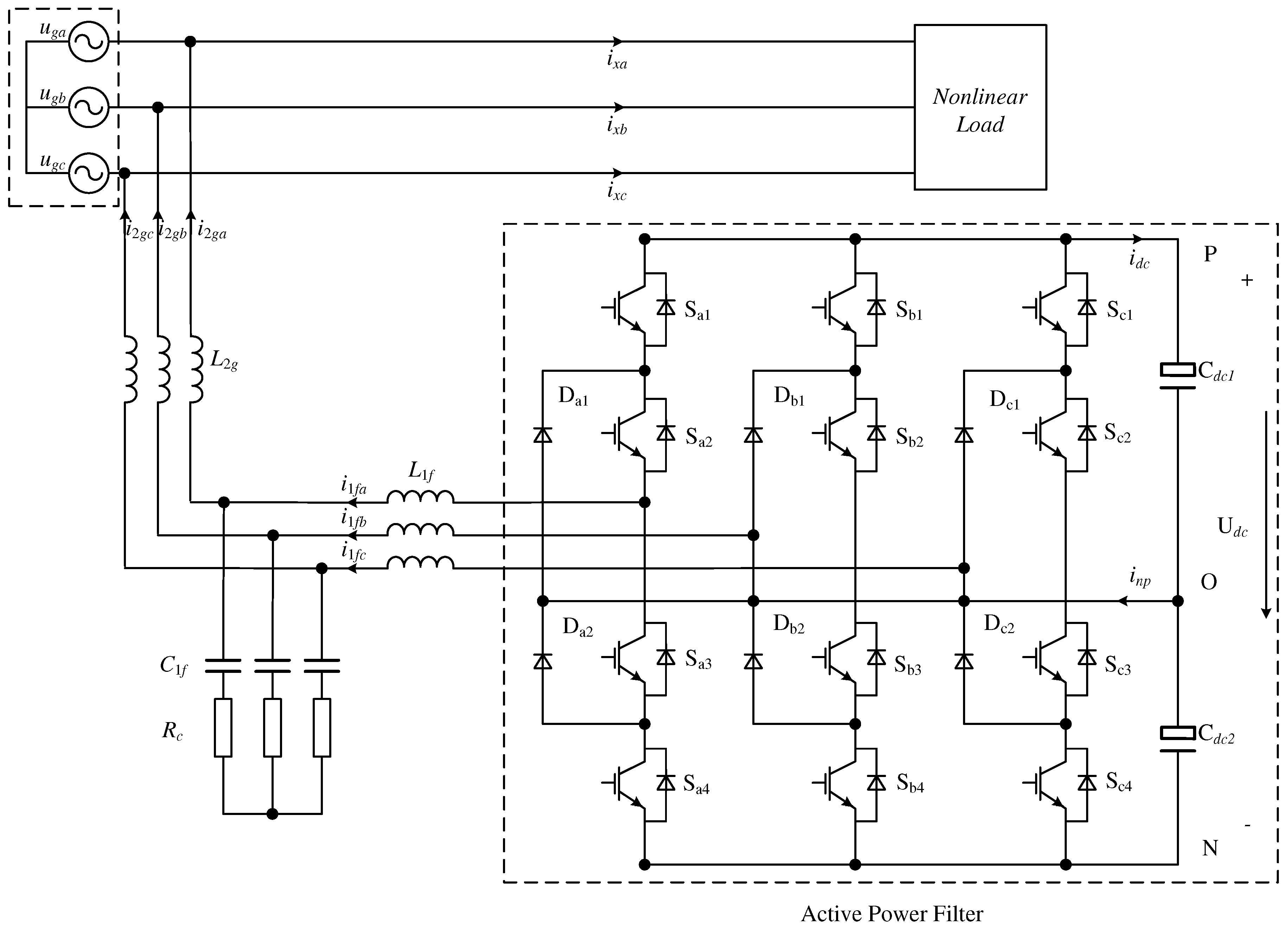
2. Mathematical Model of APF with an LCL Filter

The block diagram of the LCL APF system structure is depicted in Figure 1. The primary circuit consists of a three-level inverter and LCL filter. Within the diagram, $L_{1f}$ represents the filter inductance on the inverter side; $C_{1f}$ denotes the filter capacitance; $L_{2g}$ signifies the filter inductance on the power grid side; while $C_{dc1}$ and $C_{dc2}$ are DC side divider capacitors. Additionally, $u_{ga}$, $u_{gb}$, and $u_{gc}$ represent the three-phase grid voltage; $i_{2ga}$, $i_{2gb}$, and $i_{2gc}$ denote the current output by the inverter to the network side. Furthermore, $i_{1fa}$, $i_{1fb}$, and $i_{1fc}$ signify the APF inverter output currents; whereas $i_{xa}$, $i_{xb}$, and $i_{xc}$ represent harmonic currents.

Considering that the LCL filter may cause resonance problems, additional damping $R_c$ control is adopted to ensure system stability. Now assume: (1) three-phase power grid voltage balance; (2) filter inductance no magnetic saturation; (3) inverter switch no loss; and (4) neglecting the resistance of the filtering inductors on both sides.

Without considering $R_c$, the mathematical model of the LCL filter in the $d-q$ coordinate system can be obtained according to Kirchhoff’s laws [13]:

$$\left\{\begin{array}{c}{L}_{1f}{\displaystyle \frac{d{i}_{1fd}}{dt}}=w{L}_{1f}{i}_{1fq}-u_{cd}+u_{1fd}\hfill \\ L_{1f}{\displaystyle \frac{d{i}_{1fq}}{dt}}=w{L}_{1f}{i}_{1fd}-u_{cq}+u_{1fq}\hfill \\ L_{2g}{\displaystyle \frac{d{i}_{2gd}}{dt}}=w{L}_{2g}{i}_{2gq}+u_{cd}-u_{gd}\hfill \\ L_{2g}{\displaystyle \frac{d{i}_{2gq}}{dt}}=w{L}_{2g}{i}_{2gd}+u_{cq}-u_{gq}\hfill \\ C_{1f}{\displaystyle \frac{d{u}_{cd}}{dt}}=i_{1fd}-i_{2gd}+w{C}_{1f}{u}_{cd}\hfill \\ C_{1f}{\displaystyle \frac{d{u}_{cq}}{dt}}=i_{1fq}-i_{2gq}+w{C}_{1f}{u}_{cq}\hfill \end{array}\right.$$

(1)

where $u_{cd}$ and $u_{cq}$ represent the voltage of the filter capacitance in the d-q coordinate system. $u_{gd}$ and $u_{gq}$ stand for grid voltage.

Analysis of the LCL Filter

Considering that the three-phase parameters of the LCL filter are equal, we take one of them for analysis. Then, Figure 1 can be simplified to Figure 2.

$u_{1f}$ represents the voltage output of any phase in the three-phase inverter.

According to Kirchhoff’s laws, the relationship between the output voltage $u_{1f}$ and the inductance current $i_{2g}$ on the grid side can be obtained [21]:

$$G_{LCL}\left(s\right)={\displaystyle \frac{i_{2g}}{u_{1f}}}={\displaystyle \frac{R_{c}s+1}{L_{1f}{L}_{2g}{C}_{1f}{s}^3+(L_{1f}+L_{2g})R_c{s}^2+(L_{1f}+L_{2g})s}}$$

(2)

The third-order nature of the APF with LCL filter is evident from (2). Designing a controller for a three-level system presents significant complexity [22,23]. In fact, a lower-order model is often beneficial for the analysis and design of controllers. Therefore, this article adopts inverter side current feedback control, which helps to achieve a balance between control performance and computational complexity [24]. The transfer function of the APF output voltage $u_{1f}$ and output currents $i_{1f}$ on the inverter side is as follows [25]:

$$G_{u_{if}}\left(s\right)={\displaystyle \frac{L_{2g}{C}_{1f}{s}^2+R_c{C}_{1f}s+1}{L_{1f}{L}_{2g}{C}_{1f}{s}^3+(L_{1f}+L_{2g})R_c{C}_{1f}{s}^2+(L_{1f}+L_{2g})s}}$$

(3)

Without considering $R_c$, (3) can be simplified to (4) [26].

$$G_L\left(s\right)={\displaystyle \frac{i_{1f}}{u_{1f}}}={\displaystyle \frac{L_{2g}{C}_{1f}{s}^2+1}{L_{1f}{L}_{2g}{C}_{1f}{s}^3+(L_{1f}+L_{2g})s}}={\displaystyle \frac{1}{L_{1f}s}}\ast {\displaystyle \frac{s^2+w_r^2}{s^2+w_{res}^2}}$$

(4)

where $w_{res}$ represents the LCL resonant frequency, and $w_r$ represents the anti-resonant frequency of the LCL filter.

According to (4), the relative order of the controlled system can be reduced to first-order [27]. The simplified mathematical model is presented as follows [28]:

$$\left\{\begin{array}{c}{L}_{1f}{\displaystyle \frac{d{i}_{1fd}}{dt}}=u_{1fd}-u_{cd}+w{L}_{1f}{i}_{1fq}\hfill \\ L_{1f}{\displaystyle \frac{d{i}_{1fq}}{dt}}=u_{1fq}-u_{cq}+w{L}_{1f}{i}_{1fd}\hfill \end{array}\right.$$

(5)

As illustrated in (5), the system exhibits significant coupling in the $d-q$ coordinate system, and it is difficult to achieve satisfactory results by directly adopting PI control.

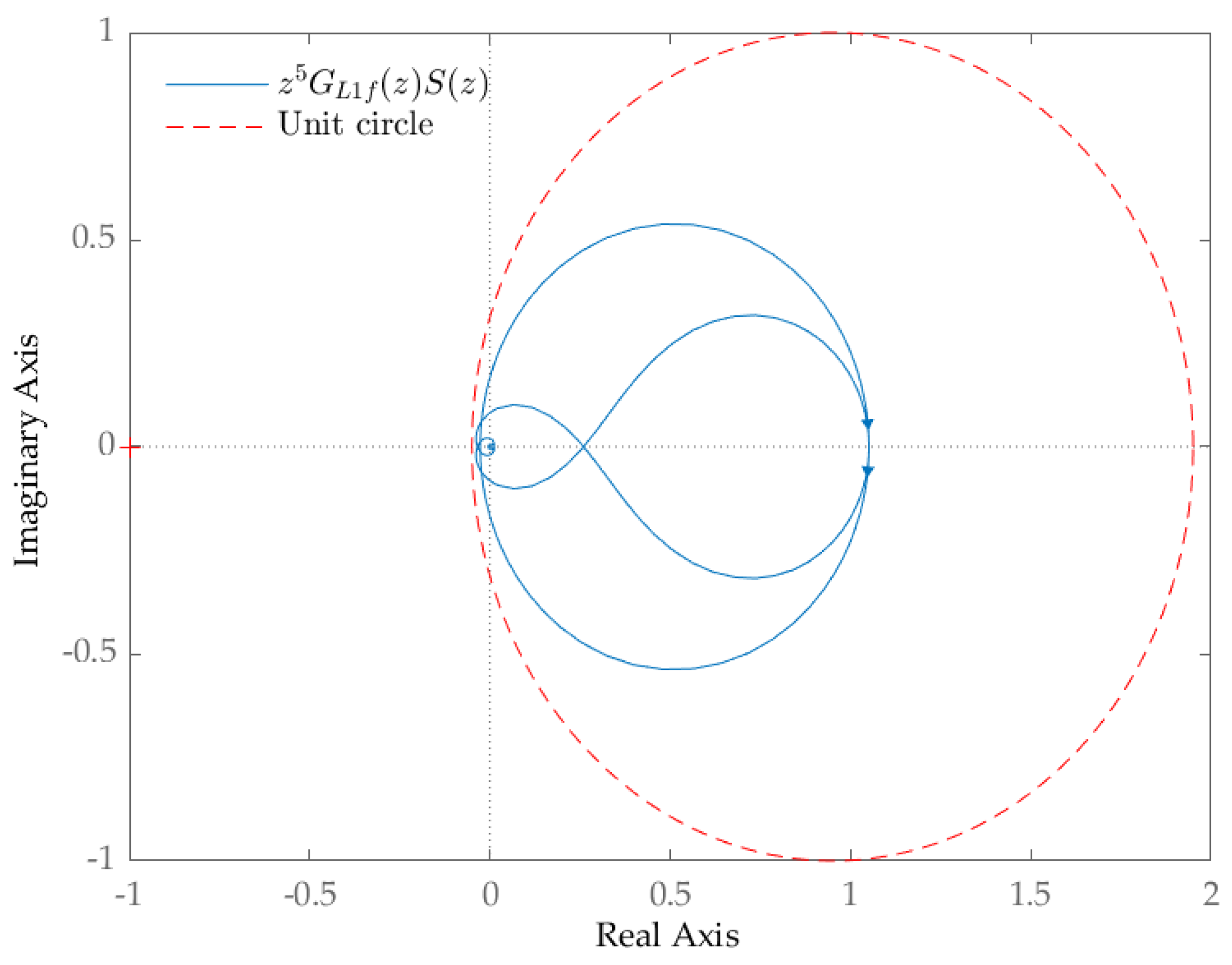
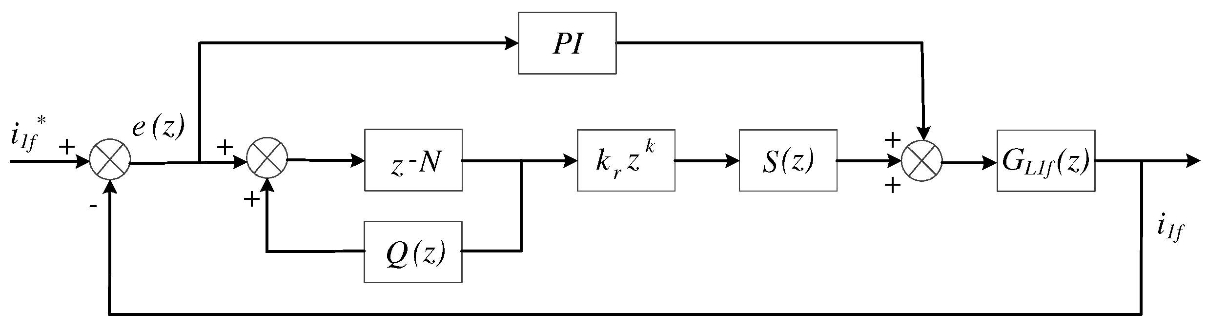
3. Current Inner-Loop Controller Design and Analysis

3.1. Design of the Repeat PI Controller

The fundamental concept of repeat control is based on the principle of internal model. This means that if the stable closed loop includes an inner model of the reference signal or disturbance signal, the system can accurately track the reference signal without steady-state error and suppress the disturbance signal. The poles of the ideal internal model are distributed on the unit circle in the z domain, but this may lead to poor system stability and potential oscillations when there are changes in the controlled object. In order to ensure system stability, a specific form of internal models is commonly utilized [29].

$$G_n\left(z\right)={\displaystyle \frac{1}{1-z^{-N}}}$$

(6)

where N represents the number of sampling points within a fundamental period.

The repeat control block diagram is shown in Figure 3, and it consists of three parts: the internal model of system, the delay link, and the compensation link.

$Q\left(z\right)z^{-N}$ is the internal model of the system, which affects the steady-state accuracy of the system. Increasing $Q\left(z\right)$ can lead to an increase in controller gain, but it may also result in decreased system stability. Typically, a constant less than 1 is used. In this paper, it uses $Q\left(z\right)=0.95$; $K_r{z}^{k}S\left(z\right)$ represents the compensator; $K_r$ denotes the repeat control gain with $K_r=1$; $z^k$ is the lead link, and it is utilized for phase lag compensation; and $S\left(z\right)$ is a second-order low-pass filter, which is employed to correct the middle and low frequency band of the control object to achieve 0dB and ensure system stability. Its continuum takes on the following form:

$$S\left(s\right)={\displaystyle \frac{w_n^2}{s^2+2\zeta w_{n}s+w_n^2}}$$

(7)

In practical engineering, it is necessary to filter out harmonics with a power frequency of less than 50 times the fundamental frequency. Therefore, the break angle frequency and damping ratio of the second-order filter in this system are $w_n$ = 3 kHz and $\zeta$ = 0.707. The transfer function of the second-order low-pass filter after discrete transformation is:

$$S\left(z\right)={\displaystyle \frac{0.2789z+0.1775}{z^2-0.8073z+0.2638}}$$

(8)

After considering the damping resistance $R_c$, the transfer function of the controlled object in the system is:

$$\begin{array}{c}\hfill G_{L1f}\left(s\right)=G_{u_{if}}\left(s\right)\ast {\displaystyle \frac{K_{pwm}s}{\tau s+1}}={\displaystyle \frac{2.31\times {10}^{-12}{s}^3+2.31\times {10}^{-8}{s}^2+0.0021s}{1.1\times {10}^{-15}{s}^4+1.375\times {10}^{-11}{s}^3+1.073\times {10}^{-6}{s}^2+0.0021s}}\end{array}$$

(9)

The Bode diagram of $G_{L1f}\left(s\right)$ is shown in Figure 4. It can be seen that in the low-frequency band below 500 Hz, the amplitude is close to 0 dB. And, in the middle-frequency band from 500 Hz to 2500 Hz, the amplitudes are not zero. The phase is not zero in the middle-frequency band and low-frequency band, and there is an offset, which seriously affects the dynamic performance of harmonic compensation. To address this issue, a repeat control compensator is used to cancel out low-frequency band effects and attenuate high-frequency band effects. The phase delay of $G_{L1f}\left(z\right)$ and $S\left(z\right)$ is synthesized and corrected by the lead link $z^k$ with $k=5$.

As shown in Figure 3, the characteristic equation of the repeat control system is:

$$1-Q\left(z\right)z^{-N}+G_{L1f}\left(z\right)S\left(z\right)z^5{z}^{-N}=0$$

(10)

According to the principle of the small gain [30], it can be deduced that the stability of the system requires all eigenroots of the eigenequation to be within the unit circle on the z plane (i.e., $\left|zi\right|<1$). Then, (10) is simplified.

$$\left|Q\left(z\right)-G_{L1f}\left(z\right)S\left(z\right)z^5\right|<1$$

(11)

To further verify the stability of the control system, the Nyquist curve of $z^5{G}_{L1f}\left(z\right)S\left(z\right)$ is plotted, as shown in Figure 5.

The value of $Q\left(z\right)$ is 0.95. It can be observed from Figure 5 that the plot of $z^5{G}_{L1f}\left(z\right)S\left(z\right)$ is enclosed within a circle with a radius of 1 and a center at (0.95, 0). So, it satisfies the stability condition and indicates that the system is stable.

When repeat control is incorporated into a PI system, the corresponding block diagram for the repeat PI controller is depicted in Figure 6.

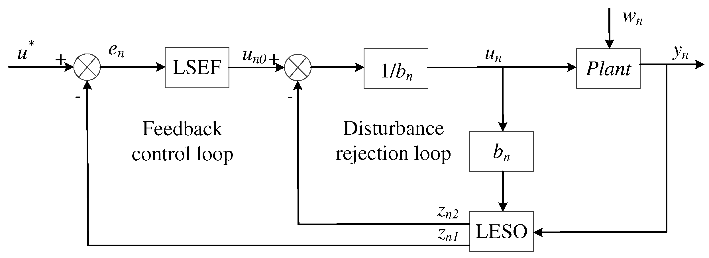
3.2. Design of the LADRC

The LADRC control system is mainly composed of two parts: an internal disturbance rejection loop and an external feedback control loop. The disturbance rejection loop is responsible for compensating the total disturbance, and its compensatory effect depends on the accurate estimation of the total disturbance by LESO [31]. The feedback control loop generates the required signal from the load, and it incorporates LSEF.

A third-order LADRC structure is relatively complex, and requires time-consuming and laborious parameter adjustments. Additionally, an accurate control object model is essential to achieve optimal control performance.

According to (4), it can be inferred that the controlled object under inverter side current feedback has a relative order of one. Therefore, this paper adopts a first-order LADRC for design, treats modeling error as internal disturbance, simplifies the control structure, and reduces tuning parameters. It is more suitable for engineering applications. The control system of the first-order LADRC is illustrated in Figure 7.

Where $u^{\ast }$ is reference signal, $y_n$ is the output current of APF, Plant represents the controlled object of the system, and $w_n$ is the unknown external disturbance.

Considering internal and external disturbances, (5) can be rewritten under LADRC framework as:

$$\left\{\begin{array}{c}{\displaystyle \frac{d{i}_{1fd}}{dt}}=b_n{u}_{1fd}+f_{nd}(i_{1fd},i_{1fq},u_{cd},w_n)\hfill \\ {\displaystyle \frac{d{i}_{1fq}}{dt}}=b_n{u}_{1fq}+f_{nq}(i_{1fd},i_{1fq},u_{cq},w_n)\hfill \end{array}\right.$$

(12)

where $b_n=1/L_{1f}$, $f_{nd}$ and $f_{nq}$ represent the total disturbance of the model, including the coupling component of the $d-q$ axis current, model-building errors and the unknown external disturbance $w_n$. Due to the analogous structure of the $d-q$ axis, for ease of description, only the d-axis is used for illustration.

Now, $y_n$ is defined as the first state variable $x_{n1}$, and the total disturbance $f_n$ is defined as the second state variable $x_{n2}$. Assuming that $f_n$ is differentiable, (12) can be rewritten in the form of a state-space equation.

$$\left\{\begin{array}{c}\dot{x_n}=A{x}_n+B{u}_i+E\dot{f_{nd}}\hfill \\ y_n=C{x}_n\hfill \end{array}\right.$$

(13)

where

$$x_n=\left[\begin{array}{c}{x}_{n1}\\ x_{n2}\end{array}\right],A=\left[\begin{array}{cc}0& 1\\ 0& 0\end{array}\right],B=\left[\begin{array}{c}{b}_n\\ 0\end{array}\right],C=\left[\begin{array}{cc}1& 0\end{array}\right],E=\left[\begin{array}{c}0\\ 1\end{array}\right],u_i=u_{1fd}$$

3.2.1. Design of LESO

In accordance with (13), the corresponding second-order LESO can be formulated:

$$\dot{z_n}=(A_n-L{C}_n)z_n+B_n{u}_n+LC{x}_n$$

(14)

where

$$z_n=\left[\begin{array}{c}{z}_{n1}\\ z_{n2}\end{array}\right],A_n=A,B_n=B,C_n=C,L=\left[\begin{array}{c}{\beta }_1\\ {\beta }_2\end{array}\right],u_n=u_{1fd}$$

and $z_{n}1$ and $z_{n}2$ represent the observed current and total disturbance on the d-axis inverter side, it utilizes for tracking $y_{nd}$ and $f_{nd}$, respectively. ${\beta }_1$ and ${\beta }_2$ denote observer gains.

The convergence rate of the observer is determined by the eigenvalue of $A_n-L{C}_n$. All observer eigenvalues are arranged at $-w_0$ [32], and then the system observation error will converge to zero.

$$\left|\lambda I-(A_n-L{C}_n)\right|={(\lambda +w_0)}^2$$

(15)

where $w_0$ is the observer bandwidth.

Substituting (14) into (15) gives

$$\left\{\begin{array}{c}{\beta }_1=2w_0\hfill \\ {\beta }_2=w_0^2\hfill \end{array}\right.$$

(16)

3.2.2. Design of LSEF

LSEF can be expressed as

$$u_n={\displaystyle \frac{u_{n0}-f_{nd}}{b_n}}$$

(17)

where $u_{n0}$ is the control quantity before disturbance compensation. When the estimation error of the total disturbance $f_n$ is ignored, the system can be simplified to an integral series structure:

$$\dot{y_n}=u_{n0}+f_{nd}-z_{n2}\approx u_{n0}$$

(18)

The integral series structure can be effectively regulated by using the linear proportional controller in the following form. This can ensure steady-state performance while avoiding the introduction of integration steps.

$$u_{n0}=k_p(v_n-z_{n1})$$

(19)

where $v_n$ is the input reference signal and $k_p$ is the controller gain.

By substituting (19) into (18), we can obtain the closed-loop transfer function from reference input to closed-loop output as

$$G_{vy}\left(s\right)={\displaystyle \frac{k_p}{s+k_p}}$$

(20)

From (20), upon compensating for the total disturbance, the system can be considered equivalent to a first-order low-pass filter. Let the controller bandwidth $w_c=k_p$, $w_c=({\displaystyle \frac{1}{10}}-{\displaystyle \frac{1}{3}})w_0$.

3.3. Design of the Repeat PI–LADRC

The block diagram of the repeat PI–LADRC decoupling control is depicted in Figure 8. The repeat PI controller offers feedback control to stabilize the system and rectify periodic errors in the stable closed loop; thereby, it can enhance the tracking accuracy of the system. The LADRC controller is employed to attenuate disturbances, including inverter-side current feedback errors, model simplification errors, d-q axis coupling effects and external unknown disturbances. Thus, it can improve the robustness and performance of the system and enhance the harmonic compensation effect of APF.

4. Voltage Outer-Loop Design and Analysis

A well-designed voltage outer loop can effectively mitigate voltage fluctuation and enhance the harmonic compensation effect of APF. The conventional DC-side voltage regulation method typically employs PI control, which is straightforward to implement and capable of effectively managing DC-side voltage. However, its dynamic adjustment ability is limited when APF is connected to the grid. To further enhance the control performance of the voltage outer loop, a composite control incorporating LADRC is introduced. Considering that the microcomponent of LSEF is generated by LESO observation and entails certain delay, a PI and LESO control structure is adopted to replace LSEF with PI. The block diagram for the PI and LESO control is depicted in Figure 9.

The DC-side voltage state equation is established as follows [33]:

$$\left\{\begin{array}{c}\dot{x_{d1}}=x_{d2}+b_d{u}_d\hfill \\ x_{d2}=h\hfill \\ y_d=x_{d1}\hfill \end{array}\right.$$

(21)

Let $x_{d1}=U_{dc}$ and $x_{d2}=f_d$, where $x_{d1}$ and $x_{d2}$ represent the state variables, and $f_d$ denotes the system disturbance. Consequently, the second-order LESO is established based on the DC voltage control model is as follows.

$$\left\{\begin{array}{c}\dot{z_{d1}}=z_{d2}-{\beta }_3(z_{d1}-y_d)+b_d{u}_d\hfill \\ \dot{z_{d2}}=-{\beta }_4(z_{d1}-y_d)\hfill \\ u_d={\displaystyle \frac{u_{d0}-z_{d2}}{b_d}}\hfill \end{array}\right.$$

(22)

where reference value $U_{d0}$ represents the output of PI controller. The observers $z_{d1}$ and $z_{d2}$ represent $x_{d1}$ and $x_{d2}$. Additionally, ${\beta }_3=2w_0^{\prime }$ and ${\beta }_3={w_0^{\prime }}^2$ are observer feedback gain matrices.

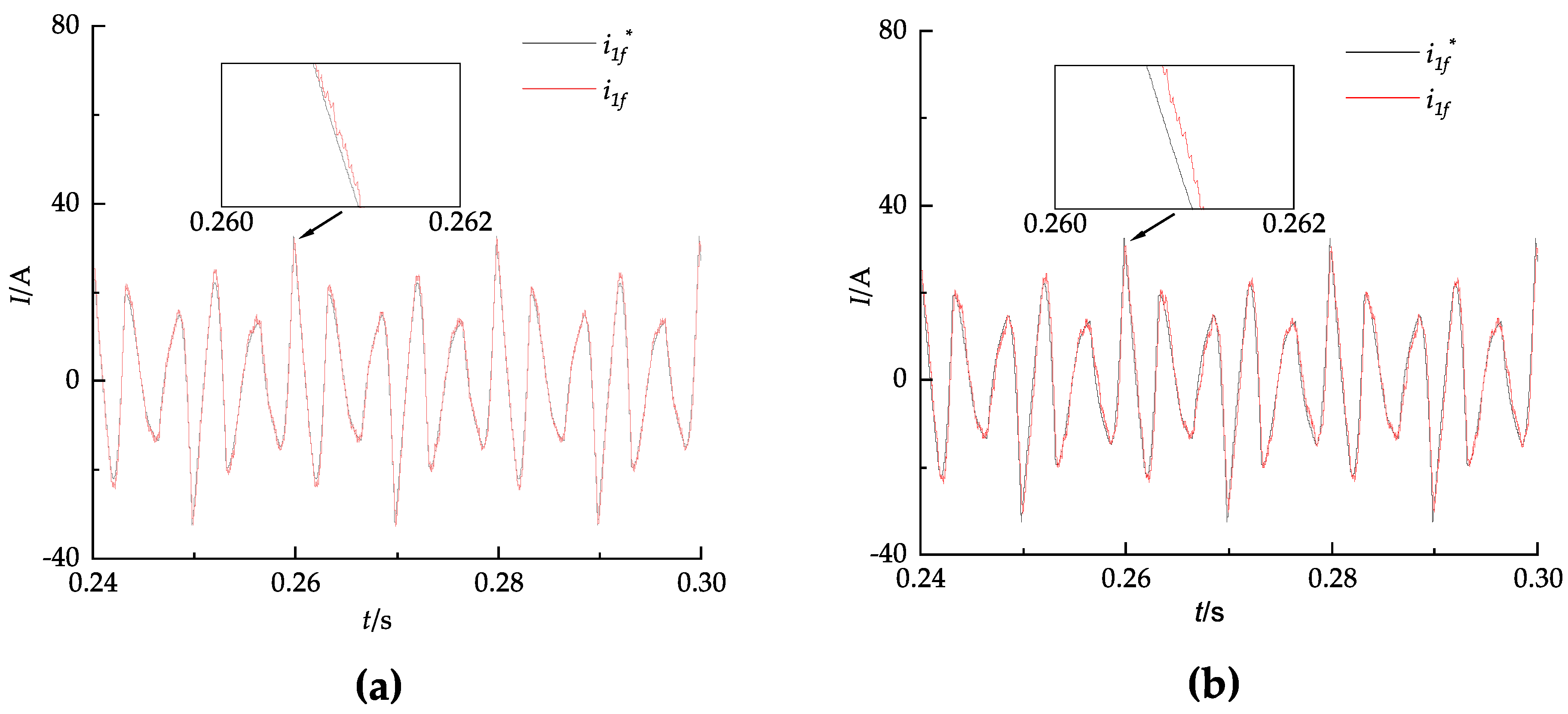
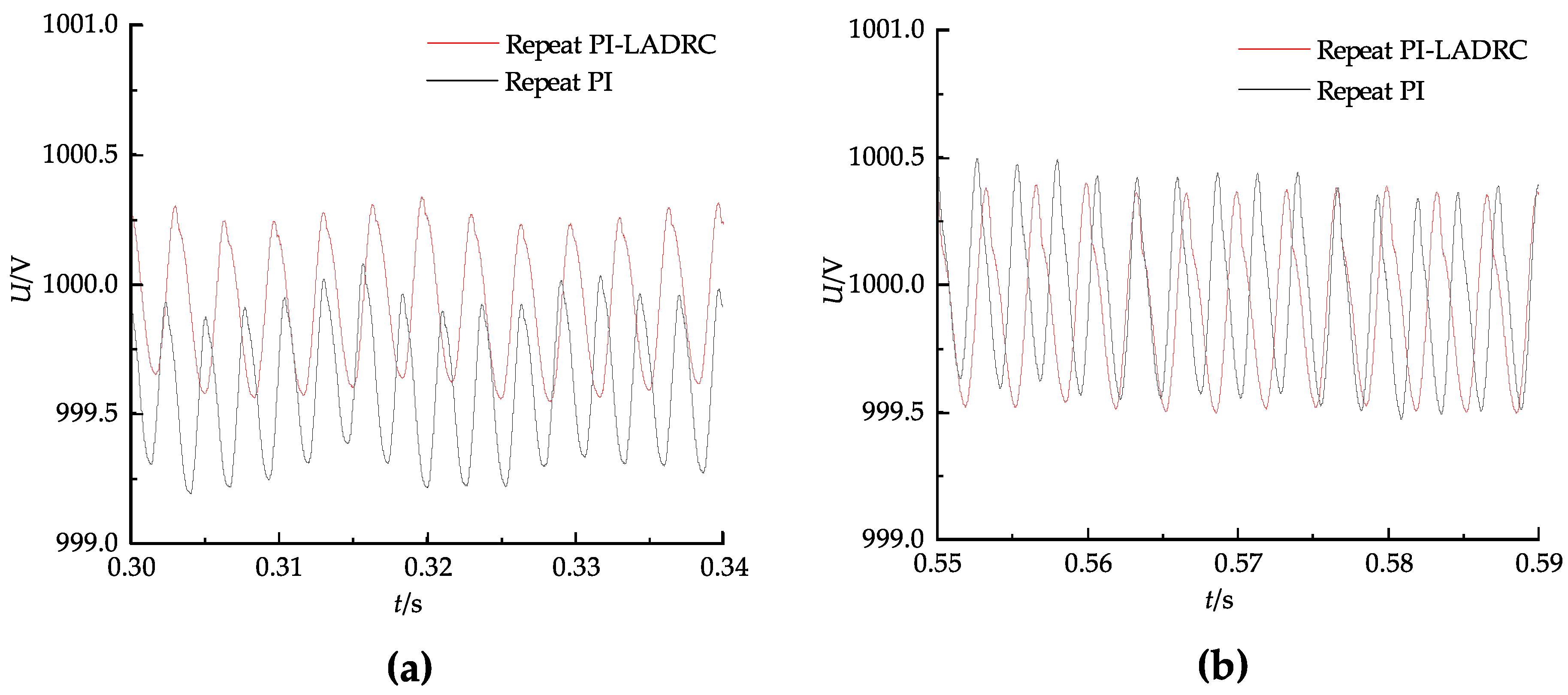
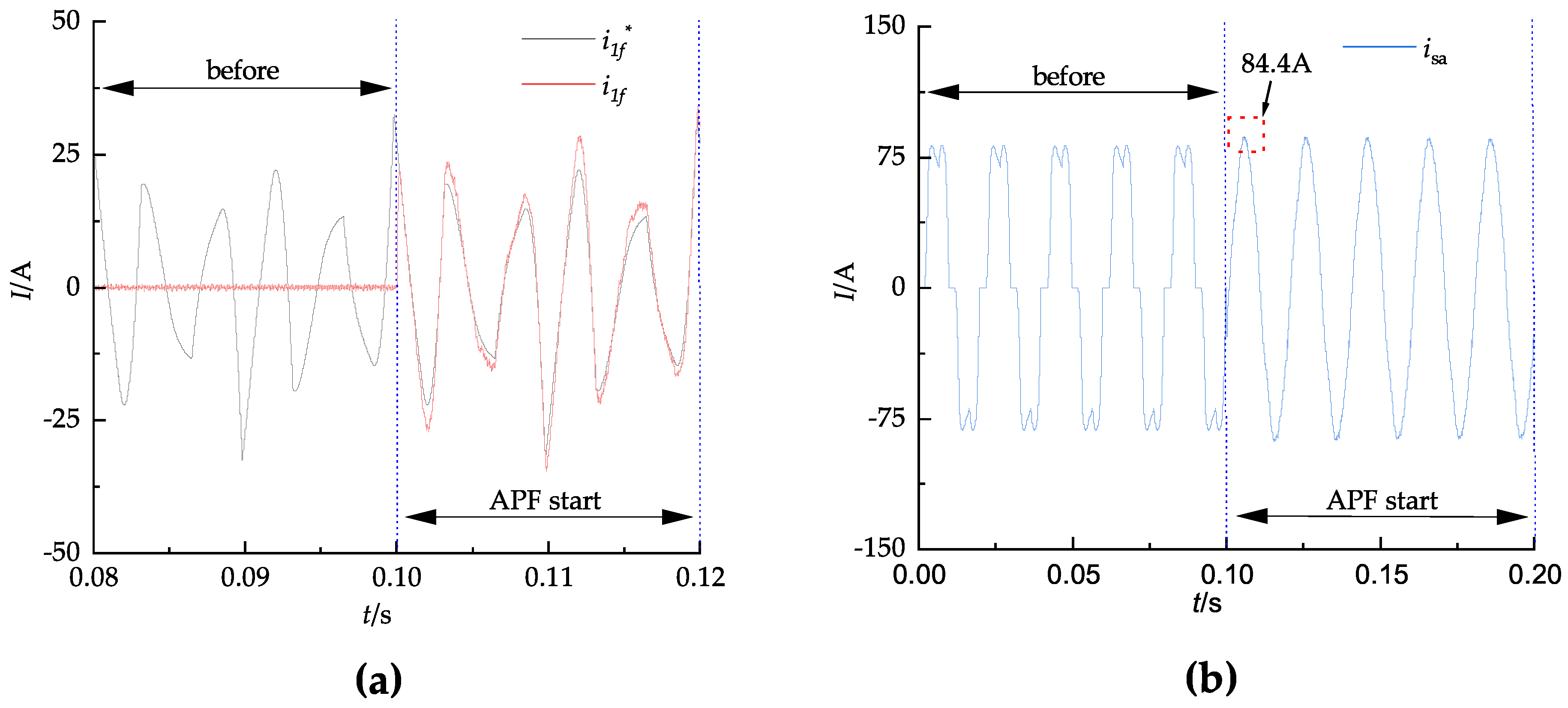
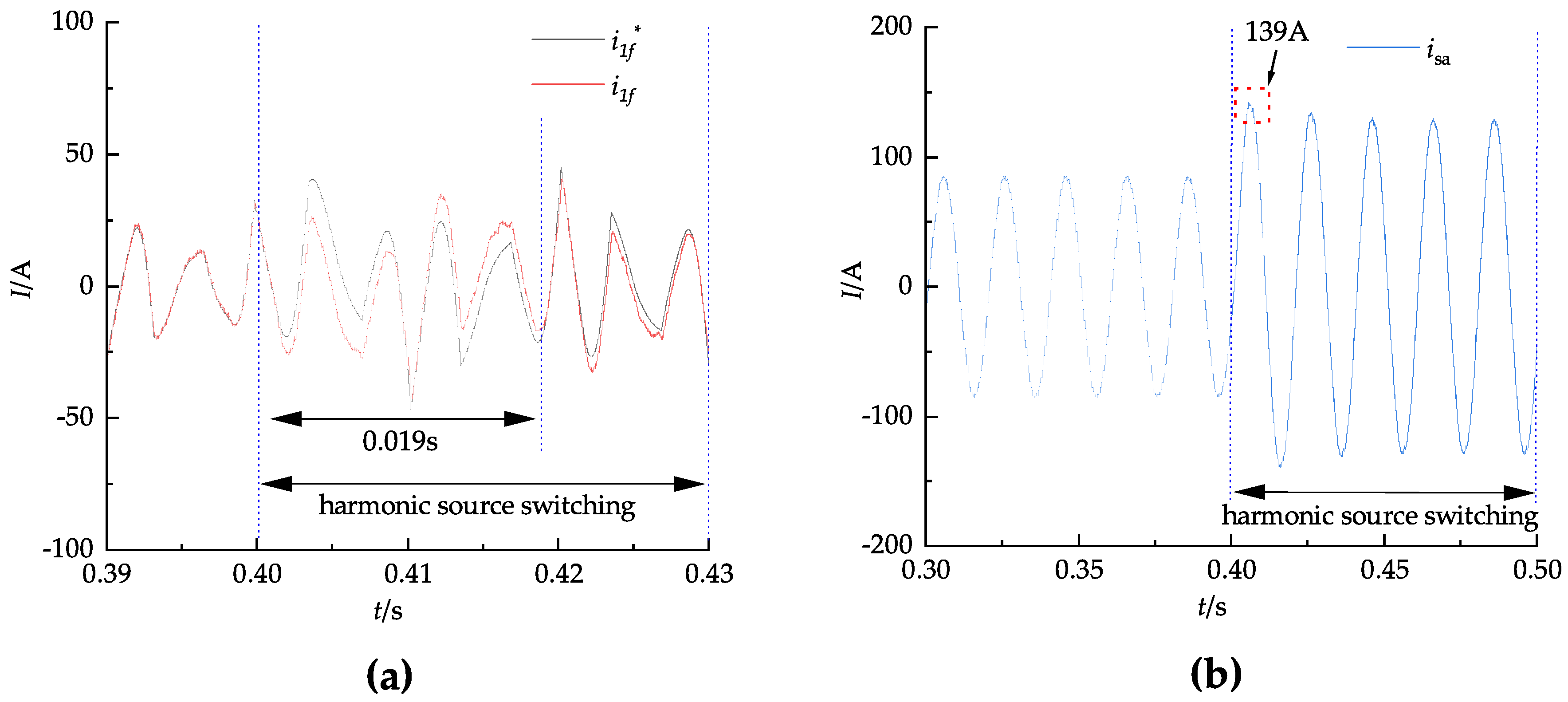
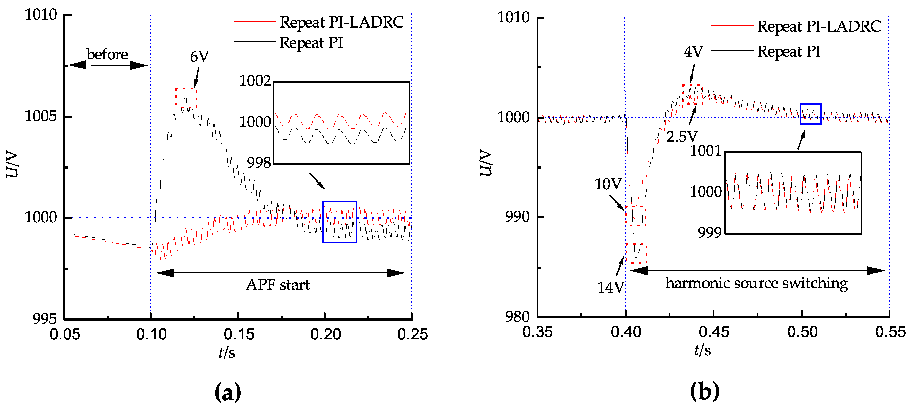
5. Simulation Verification

To validate the accuracy and feasibility of the control strategy proposed in this study, a simulation model of NPC APF is established by using MATLAB/Simlink 2022b, and the specific parameters are shown in

Table 2. Simulation parameters of the APF system.

Parameters	Numerical Value	Parameters	Numerical Value
Grid voltage	480 V	DC-side capacitance	23.5 mF
Inverter side inductance	2 mH	Switching frequency	20 kHz
Grid-side inductance	0.1 mH	Maximum compensation current	150 A
Filter capacitance	11 uF	$b_n$	400
DC-side bus voltage	1000 V	$w_c$	1000
Grid frequency	50 Hz	$w_0$	3000
$b_d$	40	$w_0^{\prime }$	1

.

In the same simulation environment, and with identical simulation parameters, a double closed-loop control system with a feedforward decoupling control for decoupling, a repeat PI control for the current inner loop, and a PI control for the outer voltage loop is chosen as the reference for comparison. To simultaneously evaluate the steady-state and dynamic control performance of these two strategies, APF is initiated at 0.1 s for harmonic suppression, and switches the harmonic load at 0.4 s (resulting in a sudden increase in load current). Taking phase a as an example, the simulation graphs are depicted in Figure 10, Figure 11, Figure 12, Figure 13, Figure 14, Figure 15 and Figure 16.

Firstly, a steady-state analysis is conducted. As shown in Figure 10, in the steady-state phase, both control strategies effectively track the harmonic current, and there are no significant differences in tracking performance. Furthermore, it can be known from Figure 11a that when the compensation current of the APF system is stable at 84 A, the DC-side potential using the repeat PI–LADRC decoupling control strategy fluctuates within the range of ±0.5 V, while the traditional repeat PI control fluctuates within the range of −1 V to +0.5 V. And, from Figure 11b, it can be known that when the compensation current is stable at 129 A, the steady-state fluctuations of the DC voltage of the two control strategies are almost the same, both within the range of ±0.5 V. Consequently, there is minimal percentage variation observed. The above analysis indicates that during steady-state control processes, the performance difference between traditional repeat PI control and repeat PI–LADRC decoupling control in harmonic current tracking and DC voltage regulation is very small; however, repeat PI–LADRC decoupling control holds certain advantages.

Secondly, it is analyzed from the perspective of dynamic control. It can be observed from Figure 12a and Figure 13a that, after starting APF, repeat PI control requires 0.008 s to track the command signal, whereas repeat PI–LADRC decoupling control achieves instantaneous tracking during implementation. As depicted in Figure 12b and Figure 13b, adoption of repeat PI control results in excessive power grid current, and the compensation current overshoot reaches 91 A. Leveraging the anti-interference capability of LADRC, repeat PI–LADRC decoupling control effectively mitigates overshoot and reduces compensated current overshoot to 84.4 A, achieving non-overshoot tracking. In Figure 16a, the difference of voltage modulation on the DC-side under different control strategies can be more clearly observed. Under repeat PI control, there is evident overshoot, while repeat PI–LADRC decoupling control can effectively mitigate overshoot and ensure smooth tracking.

Similarly, it can be observed from Figure 14 and Figure 15 that, after switching harmonic load for 0.4 s, both of them can consistently achieve harmonic current tracking within one cycle. However, the repeat PI control exhibits significant overshooting, with the compensation current overshoot reaching 153 A, whereas the repeat PI–LADRC decoupling control effectively mitigates overshoot and reduces the compensating current overshoot to 139 A. As shown in Figure 16b, it is evident that the repeated PI control results in a DC voltage drop and voltage overshoot of 14 V and 4 V, respectively; on the other hand, the repeat PI–LADRC decoupling control yields a lower DC voltage drop of 10 V and reduces voltage overshoot of 2.5 V, indicating its superior anti-interference capability.

Subsequently, the FFT analysis is used to compare and analyze the decoupling control of repeat PI–LADRC and repeat PI control in

Table 3. Comparison of harmonic current THD before and after filtering.

Load Current	84 A	129 A
Pre-compensation	22.36%	19.25%
PI control	5.15%	4.68%
repeat PI control	2.74%	2.6%
LADRC control	3.7%	3.17%
repeat PI–LADRC control	2.09%	1.69%

. At a load current of 84 A, prior to compensation, total harmonic distortion (THD) of network current stood at 22.36%. Following compensation through a repeat PI–LADRC decoupling strategy, this figure decreased significantly to just 2.09%, and makes a reduction of approximately 0.65% compared to repeat PI controller method. At a load current level of 129 A, the THD of the network current is reduced to 1.69% after repeat PI–LADRC decoupling control strategy compensation, which is 0.91% lower than repeat PI control. Table 3 also lists filtering effect of other common control strategies in two cases, and it can be observed that repeated PI–LADRC control strategy has advantages.

6. Conclusions

By establishing the LCL three-level neutral-point-clamped APF mathematical model based on inverter side current feedback control, a double closed-loop voltage-current control system is designed. The current inner loop adopts repeat PI–LADRC decoupling control to track the output current of the filter, while the voltage outer loop adopts PI and LESO control. The steady-state and dynamic characteristics are analyzed through simulation results. Compared with the traditional repeat PI control with feedforward decoupling, this strategy can effectively address the poor system tracking performance caused by sudden load changes while suppressing the distortion of grid current. It improves the current tracking effect of APF and enhances the filtering performance.

References

1. Alasali, F.; Nusair, K.; Foudeh, H.; Holderbaum, W.; Vinayagam, A.; Aziz, A. Modern optimal controllers for hybrid active power filter to minimize harmonic distortion. Electronics 2022, 11, 1453. [Google Scholar] [CrossRef]
2. Zhou, X.; Cui, Y.; Ma, Y. Fuzzy linear active disturbance rejection control of injection hybrid active power filter for medium and high voltage distribution network. IEEE Access 2021, 9, 8421–8432. [Google Scholar] [CrossRef]
3. Li, H.; Qu, Y.; Lu, J.; Li, S. A composite strategy for harmonic compensation in standalone inverter based on linear active disturbance rejection control. Energies 2019, 12, 2618. [Google Scholar] [CrossRef]
4. Das, S.R.; Ray, P.K.; Sahoo, A.K.; Ramasubbareddy, S.; Babu, T.K.; Kumar, N.M.; Elavarasan, R.M.; Mihet-Popa, L. A comprehensive survey on different control strategies and applications of active power filters for power quality improvement. Energies 2021, 14, 4589. [Google Scholar] [CrossRef]
5. Ghoudelbourk, S.; Azar, A.T.; Dib, D. Three-level (NPC) shunt active power filter based on fuzzy logic and fractional-order PI controller. Int. J. Autom. Control 2021, 15, 149–169. [Google Scholar] [CrossRef]
6. Kashif, M.; Hossain, M.J.; Zhuo, F.; Gautam, S. Design and implementation of a three-level active power filter for harmonic and reactive power compensation. Electr. Power Syst. Res. 2018, 165, 144–156. [Google Scholar] [CrossRef]
7. Hoon, Y.; Mohd Radzi, M.A.; Hassan, M.K.; Mailah, N.F. Control algorithms of shunt active power filter for harmonics mitigation: A review. Energies 2017, 10, 2038. [Google Scholar] [CrossRef]
8. Mhawi, E.; Daniyal, H.; Sulaiman, M.H. Advanced techniques in harmonic suppression via active power filter: A review. Int. J. Power Electron. Drive Syst 2015, 6, 185–195. [Google Scholar] [CrossRef]
9. Zhang, M.; Wen, J.M.; Wu, S.Y.; Guan, Y.C.; Feng, C.S.; Lu, J.H. Dual-loop control of hybrid active power filter. Electr. Mach. Control 2023, 27, 119–126. [Google Scholar]
10. Zeng, Z.; Yang, J.; Yu, N. Research on PI and repetitive control strategy for Shunt Active Power Filter with LCL-filter. In Proceedings of the 7th International Power Electronics and Motion Control Conference, Harbin, China, 2–5 June 2012; Volume 4, pp. 2833–2837. [Google Scholar]
11. Abouloifa, A.; Giri, F.; Lachkar, I.; Chaoui, F.Z.; Kissaoui, M.; Abouelmahjoub, Y. Cascade nonlinear control of shunt active power filters with average performance analysis. Control Eng. Pract. 2014, 26, 211–221. [Google Scholar] [CrossRef]
12. Li, X.; Li, B. A decoupling control method for shunt hybrid active power filter based on generalized inverse system. J. Electr. Comput. Eng. 2017, 2017, 5232507. [Google Scholar] [CrossRef]
13. Khajehoddin, S.A.; Karimi-Ghartemani, M.; Jain, P.K.; Bakhshai, A. A Control Design Approach for Three-Phase Grid-Connected Renewable Energy Resources. IEEE Trans. Sustain. Energy 2011, 2, 423–432. [Google Scholar] [CrossRef]
14. Zhou, S.; Liu, J.; Zhou, L.; Zhang, Y. DQ current control of voltage source converters with a decoupling method based on preprocessed reference current feed-forward. IEEE Trans. Power Electron. 2017, 32, 8904–8921. [Google Scholar] [CrossRef]
15. Han, J. From PID to Active Disturbance Rejection Control. IEEE Trans. Ind. Electron. 2009, 56, 900–906. [Google Scholar] [CrossRef]
16. Liu, Y.; Zeng, L.; Pan, H.; Yang, T. Research of Active Power Filter Using Improved Backstepping Active disturbance rejection control strategy. In Proceedings of the China Automation Congress, Beijing, China, 22–24 October 2021; pp. 8001–8006. [Google Scholar]
17. Gao, Z. Scaling and bandwidth-parameterization based controller tuning. In Proceedings of the American Control Conference, Denver, CO, USA, 4–6 June 2003; Volume 6, pp. 4989–4996. [Google Scholar]
18. Qin, D.; Zeng, G. Research on Parallel Shunt Hybrid Active Power Filter with repetitive LADRC algorithm. In Proceedings of the International Future Energy Electronics Conference, Taipei, Taiwan, 1–4 November 2015; Volume 6, pp. 1–6. [Google Scholar]
19. Wu, H.; Wang, Y.; Liu, B.; Chen, L.; Pei, G. Research and improvement of current control strategy of active power filter. In Proceedings of the IOP Conference Series: Earth and Environmental Science, Changchun, China, 21–23 August 2020; Volume 619, p. 012069. [Google Scholar]
20. Zhang, H.; Xian, J.; Shi, J.; Wu, S.; Ma, Z. High performance decoupling current control by linear extended state observer for three-phase grid-connected inverter with an LCL filter. IEEE Access. 2020, 8, 13119–13127. [Google Scholar] [CrossRef]
21. Feng, Z.; Zhou, X.; Wang, C.; Huang, W.; Chen, Z. LADRC-based grid-connected control strategy for single-phase LCL-type inverters. PLoS ONE 2024, 19, e0303591. [Google Scholar] [CrossRef]
22. Benrabah, A.; Xu, D.; Gao, Z. Active disturbance rejection control of LCL-filtered grid-connected inverter using Padé approximation. IEEE Trans. Ind. Appl. 2018, 54, 6179–6189. [Google Scholar] [CrossRef]
23. Zhou, X.; Xu, H.; Ma, Y.; Hu, Y. Research on Control Strategy Based on Second-order Linear Active Disturbance Rejection Control for LCL-type Grid-connected Inverter. In Proceedings of the 2022 IEEE International Conference on Mechatronics and Automation, Guangxi, China, 7–10 August 2022; pp. 864–869. [Google Scholar]
24. Xu, A.J.; Xie, B.S.; Kan, C.J.; Ji, D.L. An improved inverter-side current feedback control for grid-connected inverters with LCL filters. In Proceedings of the 2015 9th International Conference on Power Electronics and ECCE Asia, Seoul, Republic of Korea, 1–5 June 2015; pp. 984–989. [Google Scholar]
25. Pal, B.; Sahu, P.K.; Mohapatra, S. A review on feedback current control techniques of grid-connected PV inverter system with LCL filter. In Proceedings of the 2018 Technologies for Smart-City Energy Security and Power, Bhubaneswar, India, 28–30 March 2018; pp. 1–6. [Google Scholar]
26. Ming, L.; Xin, Z.; Kong, X.; Yin, C.; Loh, P.C. Power factor correction and harmonic elimination for LCL-filtered three-level photovoltaic inverter with inverter-side current control. In Proceedings of the IECON 2019—45th Annual Conference of the IEEE Industrial Electronics Society, Lisbon, Portugal, 14–17 October 2019; Volume 1, pp. 3405–3410. [Google Scholar]
27. Cai, Y.; He, Y.; Zhou, H.; Liu, Y. Active-damping disturbance-rejection control strategy of LCL grid-connected inverter based on inverter-side-current feedback. IEEE J. Emerg. Sel. Top. Power Electron. 2020, 9, 7183–7198. [Google Scholar] [CrossRef]
28. Wang, X.; Wu, C.; Pan, Z.; Tian, L. Inverter-side current control of grid-connected inverter with LCL filter based on fractional-order extended state observation. In Proceedings of the 2021 9th International Conference on Control, Mechatronics and Automation, Belval, Luxembourg, 11–14 November 2021; pp. 55–60. [Google Scholar]
29. Tang, Y.; Loh, P.C.; Wang, P.; Choo, F.H.; Gao, F.; Blaabjerg, F. Generalized design of high performance shunt active power filter with output LCL filter. IEEE Tran. Ind. Electron. 2011, 59, 1443–1452. [Google Scholar] [CrossRef]
30. Rueffer, B.S. Small-gain conditions and the comparison principle. IEEE Tran. Autom. Control 2010, 55, 1732–1736. [Google Scholar] [CrossRef]
31. Zhou, X.; Wang, J.; Ma, Y. Linear active disturbance rejection control of grid-connected photovoltaic inverter based on deviation control principle. Energies 2020, 13, 3790. [Google Scholar] [CrossRef]
32. He, G.; Chen, G.; Dong, Y.; Li, G.; Zhang, W. Research on LADRC of grid-connected inverter based on LCCL. Energies 2022, 15, 4686. [Google Scholar] [CrossRef]
33. He, Y.; Liu, J.; Tang, J.; Wang, Z.; Zou, Y. Research on control system of DC voltage for active power filters with three-level NPC inverter. In Proceedings of the 2008 Twenty-Third Annual IEEE Applied Power Electronics Conference and Exposition, Austin, TX, USA, 24–28 February 2008; pp. 1048–2334. [Google Scholar]
Figure 1. Topology of the neutral-point-clamped three-level active power filter.
Electronics 13 02973 g001
Figure 2. The principle structure diagram of the LCL filter.
Electronics 13 02973 g002
Figure 3. Block diagram of repeat control system structure.
Electronics 13 02973 g003
Figure 4. Bode diagram of the controlled object.
Electronics 13 02973 g004
Figure 5. Nyquist curve of z 5 G L 1 f ( z ) S ( z ) .
Electronics 13 02973 g005
Figure 6. The structure diagram of repeat PI.
Electronics 13 02973 g006
Figure 7. The structure diagram of LADRC.
Electronics 13 02973 g007
Figure 8. The structure diagram of repeat PI–LADRC.
Electronics 13 02973 g008
Figure 9. The structure diagram of PI and LESO.
Electronics 13 02973 g009
Figure 10. Tracking current diagram during steady-state. (a) Repeat PI–LADRC decoupling control. (b) Repeat PI control.
Electronics 13 02973 g010
Figure 11. DC-side voltage during steady-state. (a) When the load current is 84 A. (b) When the load current is 129 A.
Electronics 13 02973 g011
Figure 12. Simulation of APF startup using repeat PI control. (a) Filter tracking current. (b) Phase a grid current.
Electronics 13 02973 g012
Figure 13. Simulation of APF startup using repeat PI–LADRC decoupling control. (a) Filter tracking current. (b) Phase a grid current.
Electronics 13 02973 g013
Figure 14. Simulation of harmonic load switching for repeat PI control. (a) Filter tracking current. (b) Phase a grid current.
Electronics 13 02973 g014
Figure 15. Simulation of harmonic load switching for repeat PI–LADRC decoupling control. (a) Filter tracking current. (b) Phase a grid current.
Electronics 13 02973 g015
Figure 16. DC-side voltage. (a) Simulation at the time of APF startup. (b) Simulation at the time of harmonic load switching.
Electronics 13 02973 g016