Noncontact Rotational Speed Measurement with Near-Field Microwave of Open-Ended Waveguide

 ,
,
Abstract
:1. Introduction
2. Principle and Simulations
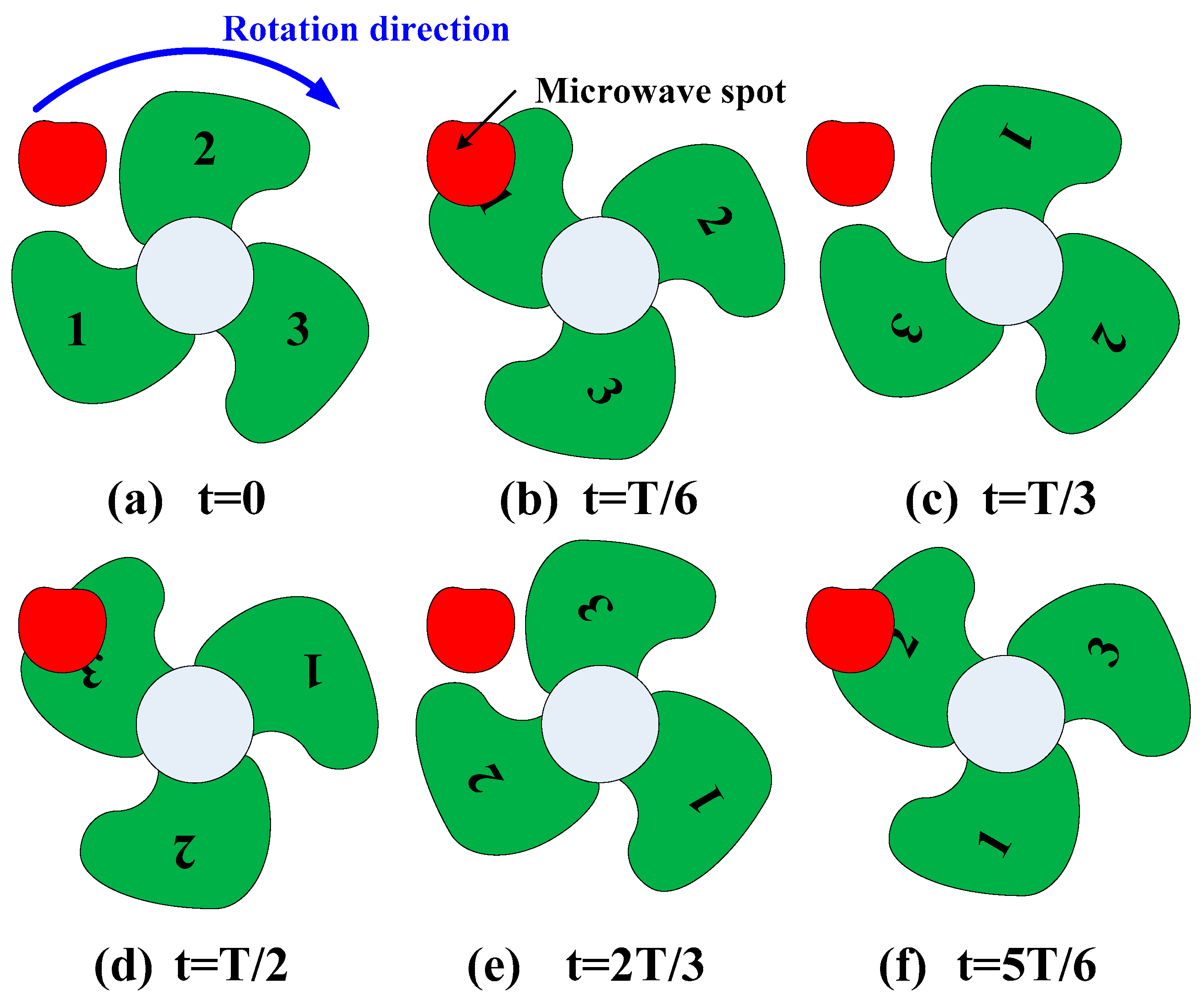
2.1. Principle of the Proposed Measurement Method
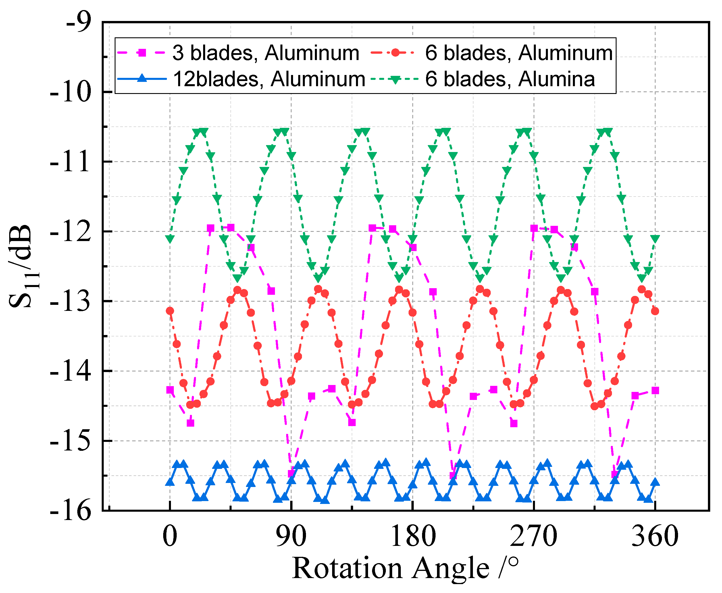
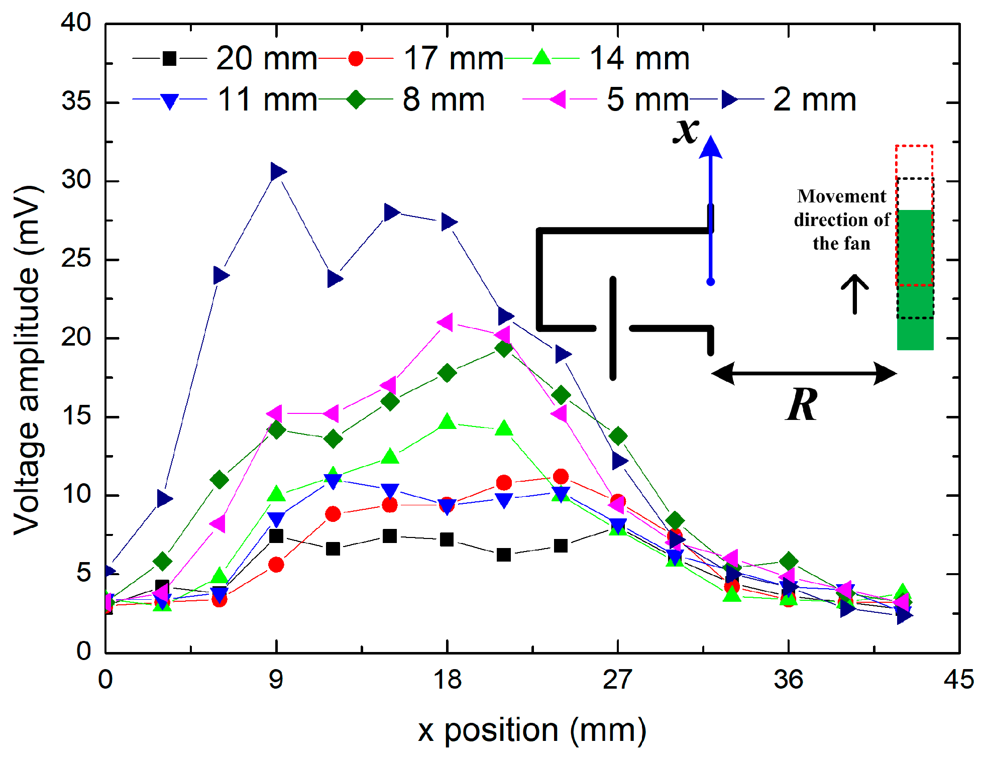
2.2. Simulations
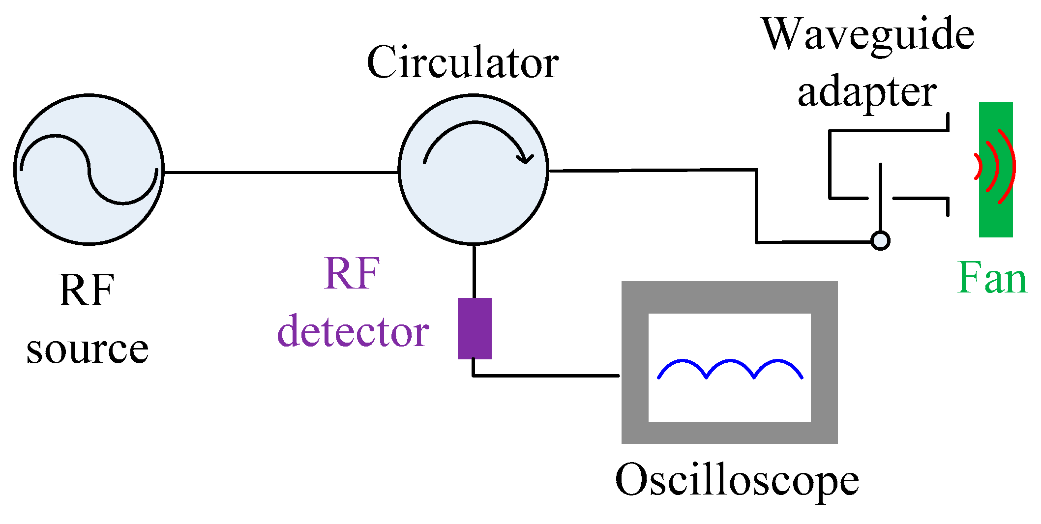
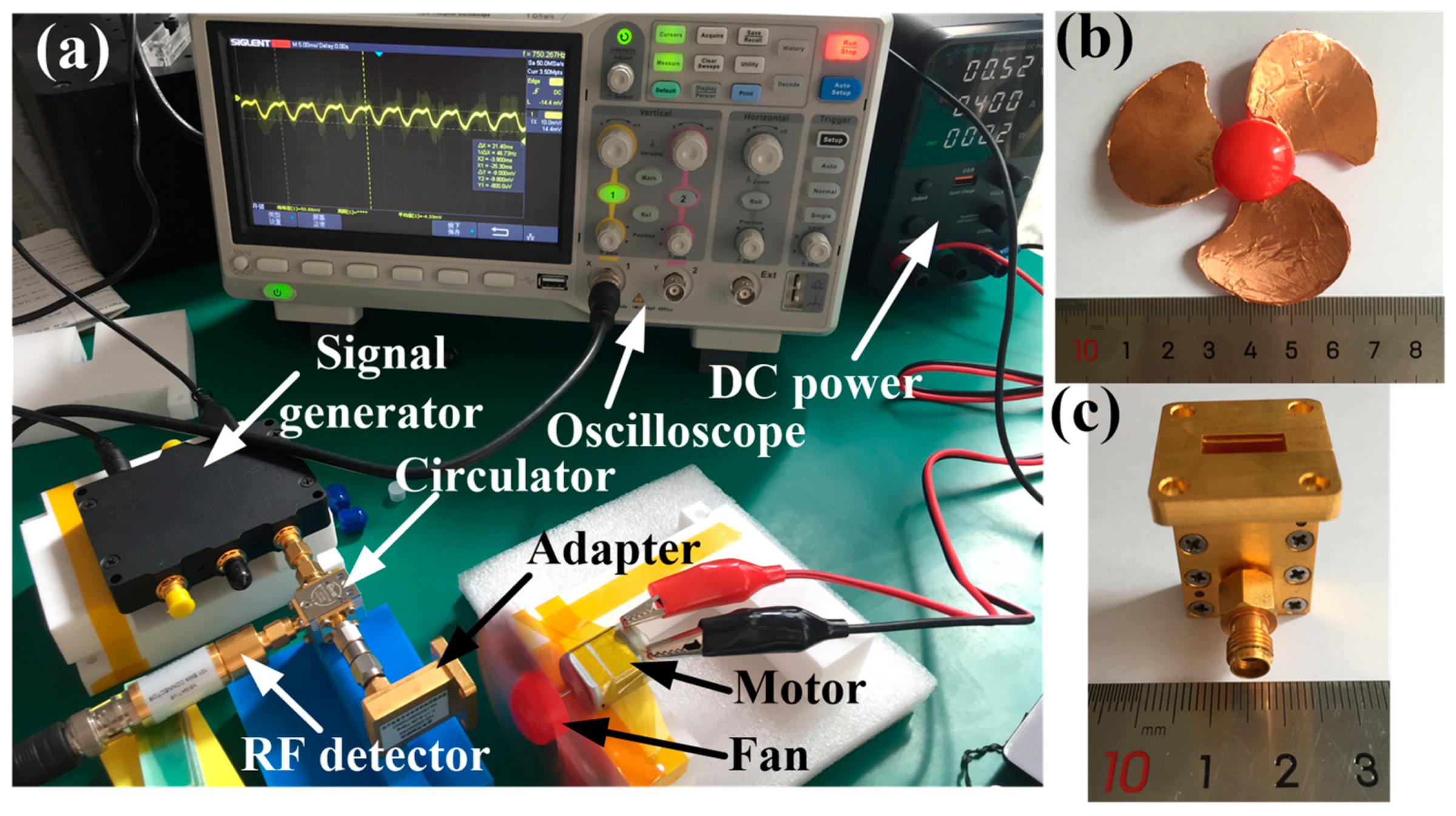
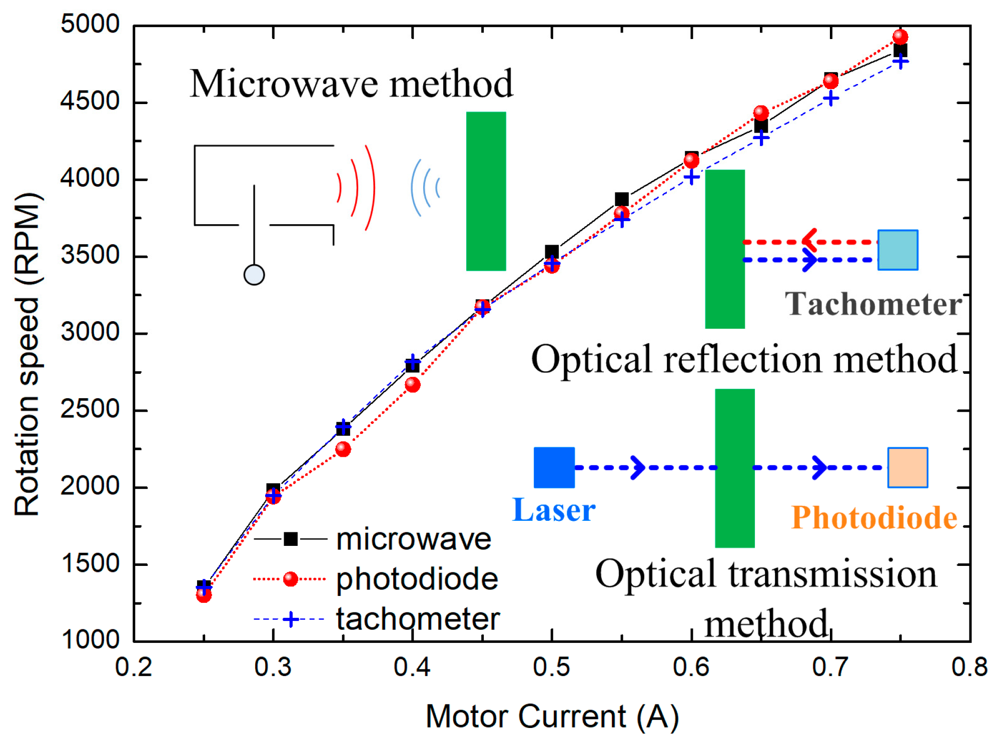
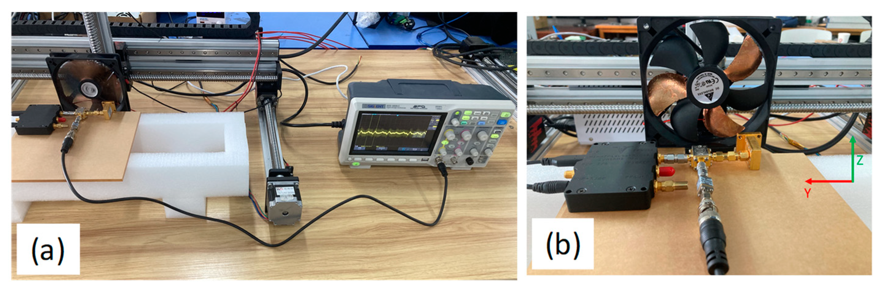
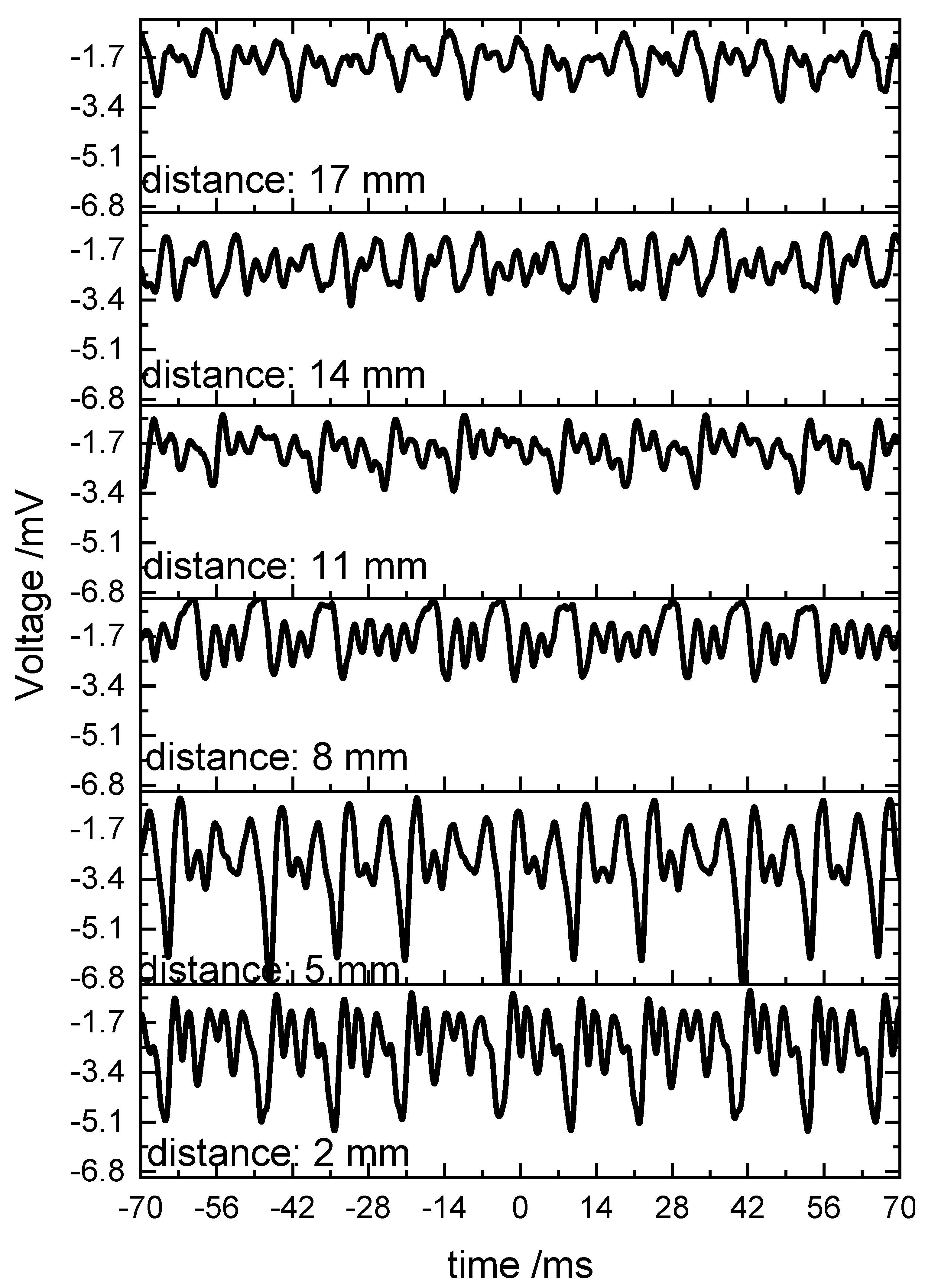
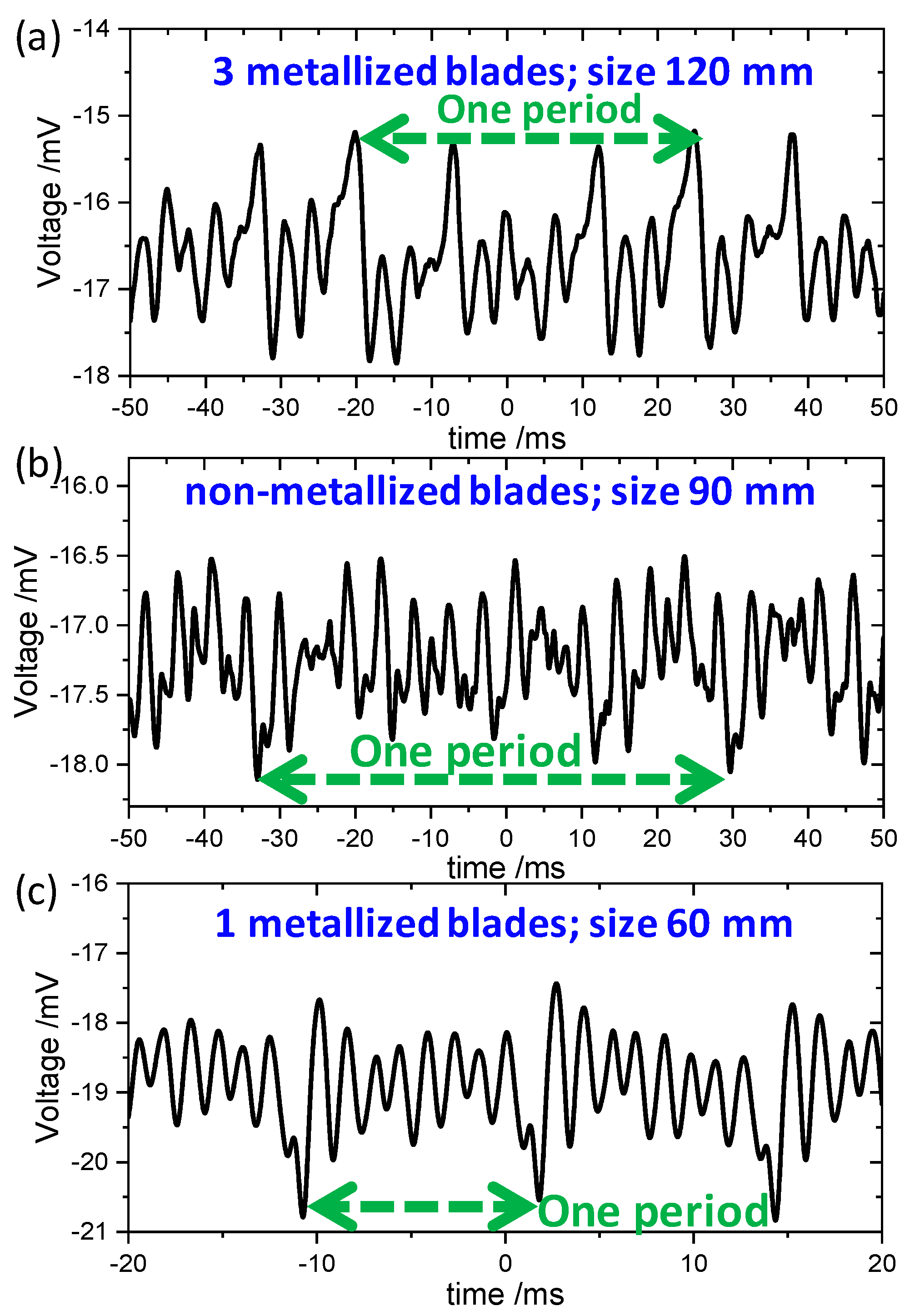
3. Experiments
4. Conclusions
Author Contributions
Funding
Data Availability Statement
Conflicts of Interest
References
- Zhou, Y.; Dong, L.; Zhang, C.; Wang, L.; Huang, Q. Rotational speed measurement based on LC wireless sensors. Sensors 2021, 21, 8055. [Google Scholar] [CrossRef] [PubMed]
- Hong, Y.; Jia, P.; Guan, X.; Xiong, J.; Liu, W.; Zhang, H.; Li, C. Wireless passive high-temperature sensor readout system for rotational-speed measurement. J. Sens. 2021, 2021, 6656527. [Google Scholar] [CrossRef]
- Hancke, G.P.; Viljoen, C.F.T. The microprocessor measurement of low values of rotational speed and acceleration. IEEE Trans. Instrum. Meas. 1990, 39, 1014–1017. [Google Scholar] [CrossRef]
- Silva, W.L.; Lima, A.M.N.; Oliveira, A. Speed estimation of an induction motor operating in the nonstationary mode by using rotor slot harmonics. IEEE Trans. Instrum. Meas. 2015, 64, 984–994. [Google Scholar] [CrossRef]
- Wang, L.; Yan, Y.; Hu, Y.; Qian, X. Rotational Speed measurement through electrostatic sensing and correlation signal processing. IEEE Trans. Instrum. Meas. 2014, 63, 1190–1199. [Google Scholar] [CrossRef]
- Fabian, T.; Brasseur, G. A robust capacitive angular speed sensor. IEEE Trans. Instrum. Meas. 1998, 47, 280–284. [Google Scholar] [CrossRef]
- Li, C.; Jia, M.; Xue, Y.; Hong, Y.; Feng, Q.; Jia, P.; Lu, H.; Xiong, J. Synchronous online monitoring of rotational speed and temperature for rotating parts in high temperature environment. IEEE Access 2021, 9, 96257–96266. [Google Scholar] [CrossRef]
- Li, K.; Li, Y.; Han, Y. A magnetic induction-based highly dynamic rotational angular rate measurement method. IEEE Access 2017, 5, 8118–8125. [Google Scholar] [CrossRef]
- Hu, X.; Tian, J. Noncontact measurement of rotational movement using IR-UWB radar. In Proceedings of the 11th International Symposium on Antennas, Propagation and EM Theory (ISAPE), Guilin, China, 18–21 October 2016. [Google Scholar]
- Varshney, P.K.; Akhtar, M.J. Substrate integrated waveguide derived novel two-way rotation sensor. IEEE Sens. J. 2021, 21, 1519–1526. [Google Scholar] [CrossRef]
- Horestani, A.K.; Shaterian, Z.; Martin, F. Rotation sensor based on the cross-polarized excitation of split ring resonators (SRRs). IEEE Sens. J. 2020, 20, 9706–9714. [Google Scholar] [CrossRef]
- Regalla, P.; Kumar, A.V.P. A fixed-frequency angular displacement sensor based on dielectric-loaded metal strip resonator. IEEE Sens. J. 2021, 21, 2669–2675. [Google Scholar] [CrossRef]
- Jha, A.K.; Lamecki, A.; Mrozowski, M.; Bozzi, M. A highly sensitive planar microwave sensor for detecting direction and angle of rotation. IEEE Trans. Microw. Theory Tech. 2020, 68, 1598–1609. [Google Scholar] [CrossRef]
- Jha, A.K.; Lamecki, A.; Mrozowski, M.; Bozzi, M. A microwave sensor with operating band selection to detect rotation and proximity in the rapid prototyping industry. IEEE Trans. Ind. Electron. 2021, 68, 683–693. [Google Scholar] [CrossRef]
- Ding, Y.; Lee, C.; Li, Y.; Wang, Z.; Li, G. An angular displacement sensor-based active feedback open complementary split-ring resonator. IEEE Microw. Wirel. Compon. Lett. 2021, 31, 1079–1082. [Google Scholar] [CrossRef]
- Jha, A.K.; Delmonte, N.; Lamecki, A.; Mrozowski, M.; Bozzi, M. Design of microwave-based angular displacement sensor. IEEE Microw. Wirel. Compon. Lett. 2019, 29, 306–308. [Google Scholar] [CrossRef]
- Chio, C.; Tam, K.; Gómez-García, R. Filtering angular displacement sensor based on transversal section with parallel-coupled-line path and U-shaped coupled slotline. IEEE Sens. J. 2022, 22, 1218–1226. [Google Scholar] [CrossRef]
- Cheong, P.; Wu, K. Full-range CSRR-based angular displacement sensing with multiport interferometric platform. IEEE Trans. Microw. Theory Tech. 2021, 69, 4813–4821. [Google Scholar] [CrossRef]
- Abdolrazzaghi, M.; Daneshmand, M. Multifunctional ultrahigh sensitive microwave planar sensor to monitor mechanical motion: Rotation, displacement, and stretch. Sensors 2020, 20, 1184. [Google Scholar] [CrossRef] [PubMed]
- Song, Z.; Wang, Q. A rotation speed measurement system based on millimeter wave. In Proceedings of the 2022 International Conference on Communications, Computing, Cybersecurity, and Informatics (CCCI), Virtual, 17–19 October 2022; pp. 1–8. [Google Scholar] [CrossRef]
- Choi, Y.; Kim, Y.; Choi, I.-S. Measurement of the rotational speed of industrial wind turbine blades using a low cost 24GHz Doppler radar. In Proceedings of the 2021 15th European Conference on Antennas and Propagation (EuCAP), Dusseldorf, Germany, 22–26 March 2021; pp. 1–5. [Google Scholar] [CrossRef]
- Ding, R.; Jin, H.; Shen, D. Rotation speed sensing with mmWave Radar. In Proceedings of the IEEE INFOCOM 2023—IEEE Conference on Computer Communications, New York, NY, USA, 17–20 May 2023. [Google Scholar] [CrossRef]


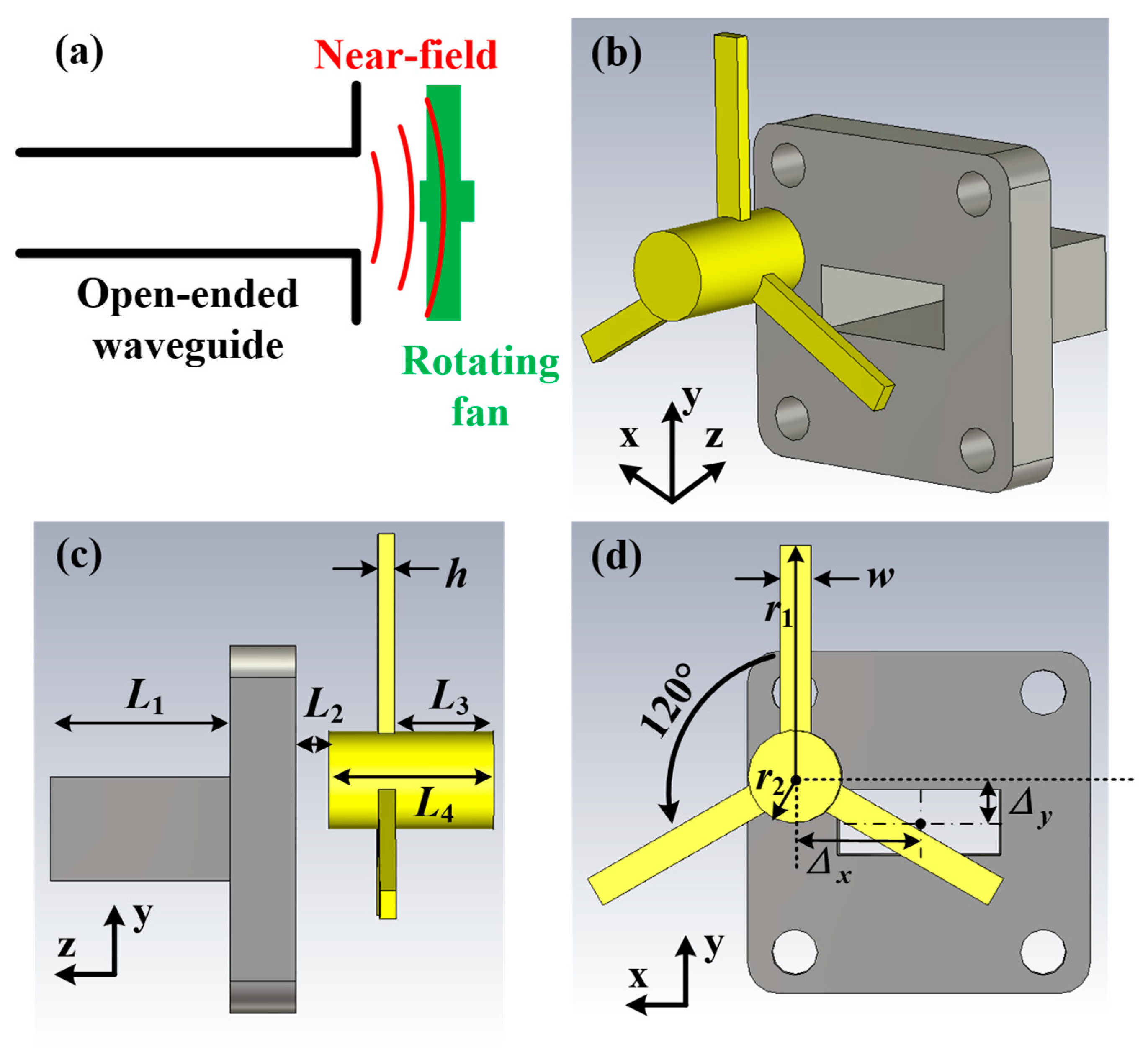
| Symbol | Values | Symbol | Values |
|---|---|---|---|
| L1 | 11.00 | w | 2.00 |
| L2 | 5.00 | r1 | 15.00 |
| L3 | 6.00 | r2 | 3.00 |
| L4 | 10.00 | Δx | 0.00 |
| h | 1.00 | Δy | 0.00 |
Disclaimer/Publisher’s Note: The statements, opinions and data contained in all publications are solely those of the individual author(s) and contributor(s) and not of MDPI and/or the editor(s). MDPI and/or the editor(s) disclaim responsibility for any injury to people or property resulting from any ideas, methods, instructions or products referred to in the content. |
© 2024 by the authors. Licensee MDPI, Basel, Switzerland. This article is an open access article distributed under the terms and conditions of the Creative Commons Attribution (CC BY) license (https://creativecommons.org/licenses/by/4.0/).
Share and Cite
Bai, Y.; Ye, M.; Yang, F.; Wang, C.; Dong, Y.; Yang, J.; Zhou, G.; Xie, Y. Noncontact Rotational Speed Measurement with Near-Field Microwave of Open-Ended Waveguide. Electronics 2024, 13, 3012. https://doi.org/10.3390/electronics13153012
Bai Y, Ye M, Yang F, Wang C, Dong Y, Yang J, Zhou G, Xie Y. Noncontact Rotational Speed Measurement with Near-Field Microwave of Open-Ended Waveguide. Electronics. 2024; 13(15):3012. https://doi.org/10.3390/electronics13153012
Chicago/Turabian StyleBai, Yongjiang, Ming Ye, Fang Yang, Chun Wang, Yingdi Dong, Jiye Yang, Guisheng Zhou, and Yongjun Xie. 2024. "Noncontact Rotational Speed Measurement with Near-Field Microwave of Open-Ended Waveguide" Electronics 13, no. 15: 3012. https://doi.org/10.3390/electronics13153012