Abstract
Network intrusion detection systems are an important defense technology to guarantee information security and protect a network from attacks. In recent years, the broad learning system has attracted much attention and has been introduced into intrusion detection systems with some success. However, since the traditional broad learning system is a simple linear structure, when dealing with imbalanced datasets, it often ignores the feature learning of minority class samples, leading to a poorer recognition rate of minority class samples. Secondly, the high dimensionality and redundant features in intrusion detection datasets also seriously affect the training time and detection performance of the traditional broad learning system. To address the above problems, we propose a deep belief network broad equalization learning system. The model fully learns the large-scale high-dimensional dataset via a deep belief network and represents it as an optimal low-dimensional dataset, and then introduces the equalization loss v2 reweighing idea into the broad learning system and learns to classify the low-dimensional dataset via a broad equalization learning system. The model was experimentally tested using the CICIDS2017 dataset and fully validated using the CICIDS2018 dataset. Compared with other algorithms in the same field, the model shortens the training time and has a high detection rate and a low false alarm rate.
1. Introduction
With the rapid development of modern computer technology and network information technology, networks affect every aspect of our lives, network attacks have become increasingly complex, and network security has never been more important. Although the Internet has brought people a lot of convenience, it also faces many new challenges. Network security problems are becoming increasingly serious, such as phishing websites, distributed denial-of-service attacks, and network worms threatening network security. Network intrusion detection systems (NIDSs) were proposed by Anderson [1] in 1980. The working principle of an intrusion detection system is mainly to monitor and filter network behaviors by analyzing host audit data, network traffic data, and other characteristics, identifying abnormal accesses in network communications, and notifying network administrators promptly, to achieve the purpose of ensuring network information security.
In recent years, due to the booming development of artificial intelligence, machine learning algorithms can better handle complex data for automated learning compared with traditional intrusion detection systems and have better adaptability and generalization. Therefore, more and more researchers have introduced machine learning technology into the intrusion detection system [2] and achieved successes [3]. However, traditional machine learning models perform poorly when dealing with complex and high-dimensional data [4], and the robustness of the machine learning model constrains the performance of the model [5]. Deep learning can automatically extract and fully learn the complex features in the data to achieve high accuracy and robustness, and thus, deep learning techniques are widely used in intrusion detection systems [6]. However, the deep learning model training process is computationally resource-intensive, with long training times and high energy consumption [7]. In addition, deep learning models are usually black-box models that lack interpretability, making it difficult to understand and explain their internal decision-making process, which hampers the performance of intrusion detection systems. Moreover, the robustness of deep learning models also constrains the security of intrusion detection systems. Abbas et al. [8] conducted an in-depth study on the robustness of the models and achieved some success. More and more scholars [9] are beginning to adopt new techniques in the field of intrusion detection.
Recently, Chen et al. [10] proposed a new randomized neural network named the broad learning system (BLS), which is based on a flat network architecture. This model is different from the extend-to-depth deep learning structure in that it does not need to use gradient descent to update the weights, and the network structure is small in size and therefore computationally faster [11]. In addition, the BLS weight update is based on pseudo-inverse operations with better model interpretability and scalability. Therefore, some people have introduced BLS into intrusion detection systems with good results [12]. However, on the one hand, NIDS datasets tend to be severely imbalanced, and traditional BLS models cannot handle imbalanced datasets well, leading to very poor detection performance for minority classes of attacks, which is fatal for intrusion detection systems detecting attacks. On the other hand, NIDS datasets tend to have high dimensionality and contain more redundant information, which can lead to more time consumption and lower detection performance of the BLS model. Therefore, certain measures must be employed to address these issues to improve the detection performance of the model.
For the problem of dataset imbalance in intrusion detection, the traditional solution is to change the number of minority class samples or majority class samples by over-sampling or under-sampling to equalize the samples. For example, the synthetic minority over-sampling technique (SMOTE) [13] increases the number of minority class samples by synthesizing new minority class samples to balance the number of samples of different classes in the dataset. However, the samples generated by SMOTE may expand the original sample space and change the distribution of the sample data, leading to poor classification or even confusion of the model in the boundary region, and often causing more time cost due to the introduction of new samples. For the problem of high dimensionality of datasets in intrusion detection, the traditional method is based on the principal component analysis (PCA) dimensionality reduction [14]. Although it can reduce the dimensionality of the dataset, as a linear dimensionality reduction method, it can only find the linear correlation structure in the data, and for the non-linear structure of intrusion detection datasets, PCA cannot effectively capture this information, and its dimensionality reduction is achieved by projecting the data to a new low-dimensional space that often results in a serious loss of information in the original data.
To address the above problems, we propose a deep belief network broad equalization learning system (DBELS), in which the deep belief network (DBN) performs data dimensionality reduction on the NIDS dataset to eliminate redundant information. The equalization loss v2 (EQL v2) idea is introduced into the BLS, and the model balances the different classes of samples by adjusting the positive and negative gradient factors to enhance the performance in detecting attack samples of minority classes and classifies low-dimensional datasets to achieve the purpose of classifying and detecting attacks. The main contributions of this paper are as follows.
- We introduce the EQL v2 idea into the BLS and propose a new model by adding positive and negative gradient factors and recalculating its weights, which improves the poor learning ability of the BLS model for minority class samples by adjusting the positive and negative gradient factors and mitigates the defect of the BLS model in that it is not good at dealing with the imbalanced dataset, to improve the performance of detecting minority class samples.
- We evaluated two types of DBN-based dimensionality reduction models—the traditional DBN model and the DeBN model that introduces the idea of EQL v2—and experimentally compared the effects of the two dimensionality reduction models on the classification effect.
- We conducted many experiments on the DBELS model based on the publicly available benchmark dataset CICIDS2017, giving detailed experimental setups including binary and multi-classification, and evaluating the model in terms of accuracy, recall, false positive rate, time, and the receiver operating characteristic curves, finding obvious advantages over other models. We also tested the effect of hyperparameters on the model through many experiments and conducted comparative analyses with other state-of-the-art models.
- We further validated the fitness and scalability of the proposed model with the CICIDS2018 dataset. The performance and usefulness of the proposed model were evaluated by comparative analysis with other models.
The rest of this paper is organized as follows: Section 2 reviews the current research on intrusion detection systems based on the BLS, data dimensionality reduction, and data imbalance. In Section 3, we describe the details of the proposed DBELS. Detailed experimental results are reported and analyzed in Section 4 and Section 5. Section 6 concludes this paper.
2. Related Works
This section focuses on the current state of research and the shortcomings of the broad learning system (BLS)-based network intrusion detection system (NIDS). We give traditional solutions to the limitations of the traditional BLS and analyze the advantages and disadvantages of these methods.
2.1. NIDS Based on BLS
The BLS model is a shallow network model that transforms and learns features by mapping nodes and enhancement nodes and calculates the model weights quickly by pseudo-inverse operations, which makes it simple and quick to train. When it was proposed, broad learning aroused widespread interest, and its applications are being investigated in many research fields, such as computer vision, image processing, medical data analysis, and natural language processing. There are also some works in the field of network intrusion detection. Li et al. [15] proposed a hybrid intrusion detection model based on the recurrent neural network (RNN) and BLS, and the experimental results show that the model based on the BLS has a better training effect and a shorter training time. Laura et al. [16] implemented the cascade of feature mapping nodes, a cascade of enhancement nodes, and a cascade of feature mapping nodes and enhancement nodes. The authors concluded that the cascade of enhancement nodes requires a longer training time than other BLS variants. Subsequently, they proposed a DDoS detection system based on broad learning for communication networks [17]. The authors concluded that the best detection performance can usually be achieved by using a cascaded BLS. Li et al. [18] proposed a tri-broad learning system (TBLS) based on the BLS model, which learns features from three dimensions of temporal granularity, data content, and spatial granularity of the dataset. Experimentally, it was proved that the TBLS model can achieve better detection performance by learning features from the three dimensions.
Although the BLS model has achieved some success in the field of intrusion detection, as a shallow neural network, it relies too much on the topology, number of samples, and class information of the training samples, and is unable to cope with imbalanced datasets. This leads to it paying too much attention to the majority class samples, and it almost ignores the learning of the minority class samples when learning classification, which leads to poor detection performance on imbalanced datasets, especially for the minority class samples, which are worse or even undetectable. Second, high-dimensional datasets increase the complexity of BLS models and increase computational and storage costs. In addition, the higher the data dimensionality, the greater the influence of noise and redundant features, which may mask useful information and reduce the accuracy and stability of the BLS model. Therefore, certain techniques are needed to adapt the BLS to imbalanced and high-dimensional datasets for intrusion detection.
2.2. NIDS Based on Data Imbalance
Data imbalance refers to the fact that in the real world, different classes of data have different distributions, where certain types of data are significantly underrepresented, which has a serious negative impact on model classification. The datasets of intrusion detection are often highly imbalanced, which is fatal to the training and detection performance of the model; for example, in the case of CICIDS2017, the normal behavior of Benign accounts for 82.248%, and the abnormal behavior of Attack accounts for only 17.752%. Attack samples of DoS/DDoS account for 14.571%, Port Scan accounts for 2.607%, Brute Force accounts for 0.389%, Web Attack accounts for 0.096%, and Botnet accounts for 0.088%; thus, it is obvious that the normal class of samples is much more than the attack class of samples, which will cause the model to learn the majority-class samples too much. In response to the imbalance of intrusion detection datasets, some scholars have already conducted in-depth studies. Wu T et al. [13] addressed imbalanced data in network intrusion detection using k-means clustering and the synthetic minority over-sampling technique (SMOTE). They clustered data, identified minority-class clusters, and applied SMOTE to generate synthetic samples, demonstrating effectiveness in experiments. Ahmad T et al. [19] developed a hybrid model combining feature selection and pattern mining. They used rule-based analysis for dimensionality reduction, SMOTE for balancing data, and adaptive boosting (AdaBoost) for learning, effectively detecting minority-class samples. With deep learning advancements, Hao X et al. [20] used GANs to create synthetic datasets, enhancing classifier performance on minority classes through realistic data generation.
However, most of the methods used to solve the data imbalance problem in intrusion detection are based on generating data, whether it is generating minority-class samples by over-sampling or reducing majority-class samples by under-sampling, which balances the different samples by changing the number of the dataset; however, this changes the data distribution of the original data, which may affect the model’s effect of learning to classify the dataset. In addition, the over-sampling method will increase the number of datasets, which will increase the extra computational cost of the model and cause extra time consumption. In recent years, Jin et al. [21] proposed equalization loss v2 (EQL v2), which is guided by positive and negative gradients and re-adjusts the weights to balance the learning of each type of task and enhance the learning of minority-class samples, and has achieved certain results. Since it does not change the distribution and number of the original samples and adjusts the weights so that the model learns each class of samples in a more balanced way, this is of great significance for solving the imbalance problem of intrusion detection systems, and introducing this idea into the BLS is conducive to enhancing the detection performance of the model in the face of imbalanced datasets.
2.3. NIDS Based on Data Dimensionality Reduction
Researchers have proposed some solutions to cope with the high-dimensionality problem in the field of intrusion detection. Zhang B et al. [14] proposed an intrusion detection method using an enhanced principal component analysis (PCA) combined with the Gaussian plain Bayesian algorithm. By weighting the primary feature vectors in PCA, the method reduces data contamination. This approach, followed by the Bayesian algorithm for detection, significantly decreases detection time compared to using classifiers alone. Shen Z et al. [22] introduced an enhanced naive bayes classification algorithm that integrates principal component analysis with linear discriminant analysis to reduce sample space dimensionality and refines Bayesian computation by incorporating attribute correlation. This approach allows the classifier to account for both attribute frequency and correlation issues, addressing real-time and accuracy challenges in intrusion detection with numerous features. Salo F et al. [23] developed a feature-processing integration technique that combines information gain and principal component analysis to extract a low-dimensional optimal subspace. They then merge multiple classifiers using support vector machines, instance learning algorithms, and multilayer perceptron decision strategies, employing a probability mean combination rule for voting. Testing across various datasets demonstrated that this method not only achieves high accuracy but also significantly reduces computational costs, making it more effective for large-scale data detection.
However, most of the current solutions to the problem of high dimensionality in NIDS datasets are machine learning algorithms, which reduce the dimensionality of the dataset to a certain extent, but still have greater limitations in the face of non-linear, high-dimensionality features, resulting in a lower detection rate of the model. Since deep learning algorithms are effective in learning high dimensionality, and non-linear features can autonomously complete the learning and feature extraction of raw data without too much human intervention, deep learning algorithms have been introduced into large-scale intrusion detection systems, which can better complete the extraction and dimensionality reduction of data features. The deep belief network (DBN), as a representative deep learning model, was proposed by Geoffrey Hinton et al. [24] in 2006. From the raw data, it can learn the multi-layered abstract feature representations that effectively capture the complex structure and changing patterns of the data. This hierarchical feature extraction process helps to map high-dimensional input data to a low-dimensional representation space while preserving the important information of the data for dimensionality reduction. Compared with traditional dimensionality reduction methods, DBN dimensionality reduction not only better maintains the structure and relevance of the data but also adaptively learns the non-linear relationships in the data, which improves the expressive ability and classification performance of the reduced data. Therefore, the DBN is superior in the task of dimensionality reduction for intrusion detection models.
3. Methodology
This section constructs the deep belief network broad equalization learning system (DBELS) based on BLS, EQL v2, and DBN in detail in three stages: data preprocessing, data dimensionality reduction, and model classification.
3.1. DBELS Architecture
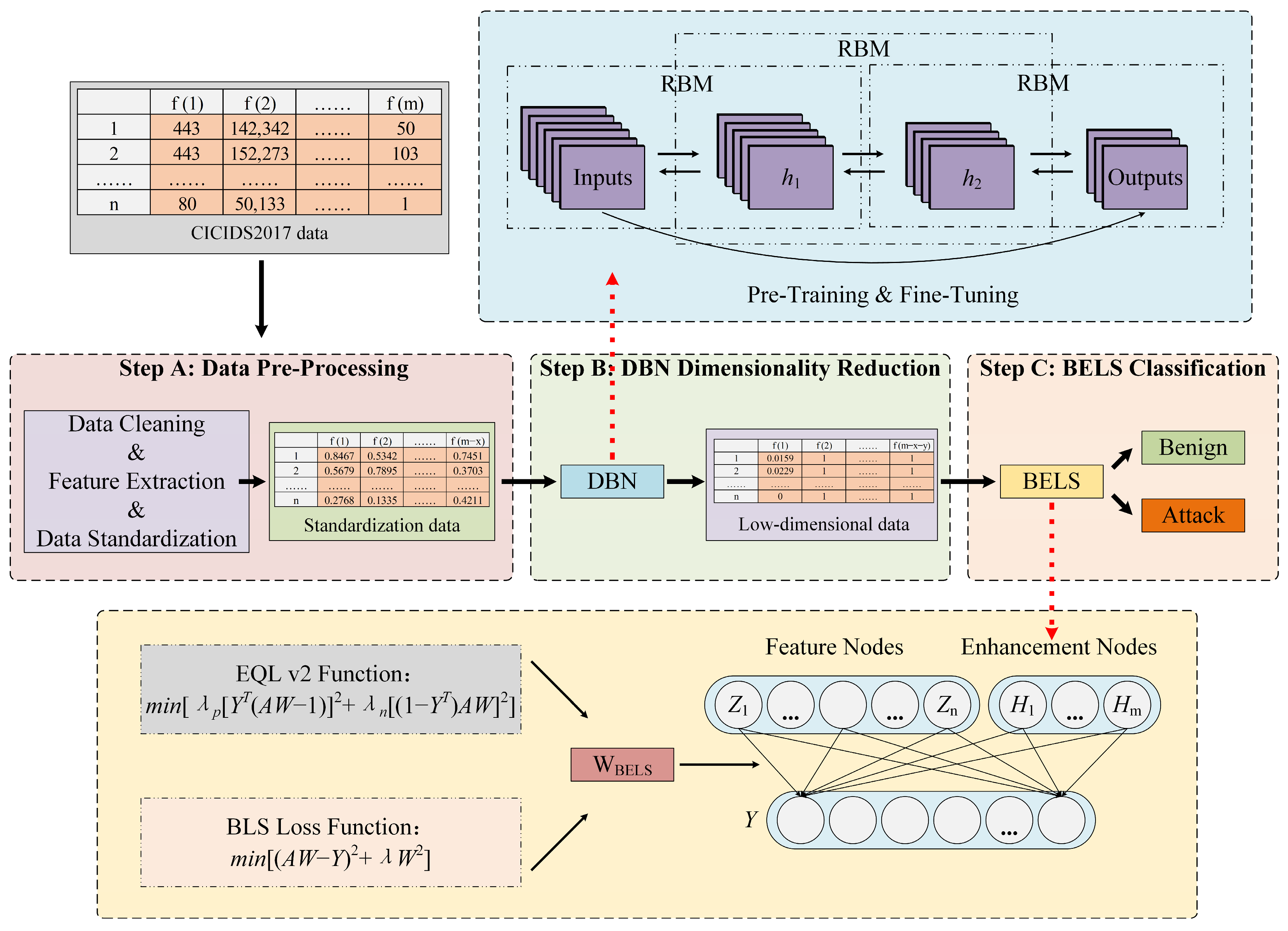
The framework of DBELS is shown in Figure 1, which is divided into three stages. The first stage is data preprocessing, which mainly processes the original data into a data form suitable for the dimensionality reduction of the DBN. The CICIDS2017 dataset contains 79 features containing many redundant features that hamper the model training and classification. In this paper, data preprocessing includes two parts: data cleaning and data standardization. The purpose of data cleaning is to reduce redundant features by calculating the contribution of features to the classification through correlation coefficients, eliminate the bad values of the data, and avoid its negative interference effect on the model. The purpose of data standardization is to make the model focus on different features of the data in a balanced way, while ignoring the influence of features with different weights on the model due to the size of the value. Due to the serious data imbalance in the CICIDS2017 dataset, the over-sampling method SMOTE can be used to increase the minority attack samples when the DBN reduces dimensionality to alleviate the problem of too few samples for the minority class.
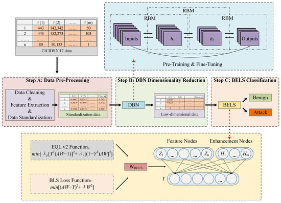
Figure 1.
The structure of DBELS.
The second stage is DBN dimensionality reduction, which aims to represent the original high-dimensional data as optimal low-dimensional data. The DBN dimensionality reduction model we use adopts a classic structure, which maximizes the retention of core features while reducing the feature dimensions as much as possible. The model fully trains each restricted Boltzmann machine (RBM) through pre-training, adjusts the whole DBN structure through weight fine-tuning, and fully learns the features of the standardized dataset, which is represented as an optimal low-dimensional dataset. The third stage uses the broad equalization learning system (BELS) to classify the optimal low-dimensional data. The BELS model equalizes the model’s learning of the minority-class samples by adjusting the positive and negative gradient factors and increasing its weights to enhance the detection and recognition class of the minority-class samples.
3.2. Deep Belief Network
3.2.1. Restricted Boltzmann Machine
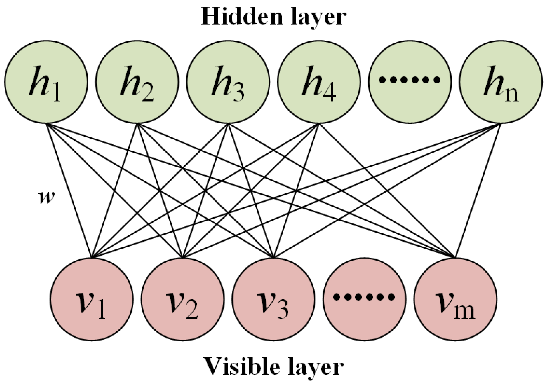
The restricted Boltzmann machine [24] is the basic structure of the DBN, which is a shallow neural network and consists of a two-layer structure of visible and hidden layers. Connections in an RBM are undirected, and there are no connections between neurons in the same layer; its structure can be seen in Figure 2. Commonly used RBMs are generally binary. Whether they are in the hidden layer or the visible layer, their neuron takes the value of 0 or 1 only. The working principle of an RBM is based on the energy function, and the energy function of the visible layer and hidden layer are given by
where belongs to the visible layer and belongs to the hidden layer, and are model biases, is weight of the model, the first part represents the contribution of the nodes of the visible layer to the energy of the system, the second part represents the contribution of the nodes of the hidden layer to the energy of the system, and the last part represents the contribution of the energy of the system due to the interaction between the visible layer and the hidden layer.
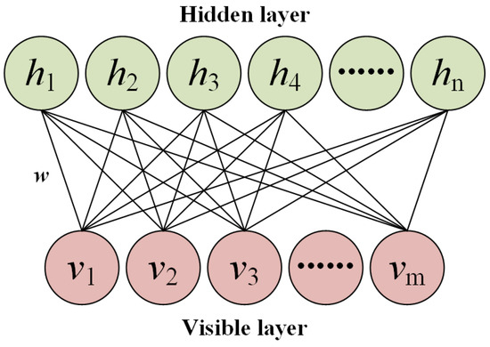
Figure 2.
The structure of RBM.
The RBM defines the joint probability density of the visible and hidden layers in terms of an energy function. The joint probability of the visible layer and hidden layer is given as
where is the partition function, which is used to normalize the probability distribution and ensure that the sum of the probability distributions is equal to 1:
With the joint probability density of the visible and hidden layers, summing over yields the marginal density distribution of the visible layer:
During the RBM model training process, the hidden layer variable is sampled and computed using the posterior probability , and the new visible layer variable is sampled by the posterior probability ; subsequently, the new hidden layer variable is sampled again in a repetitive manner to obtain the visible layer . The above steps are repeated several times until the parameters converge or reach the predefined number of iterations, the joint probability distribution is close to the smooth distribution, and the RBM training is completed.
3.2.2. Training of Deep Belief Network
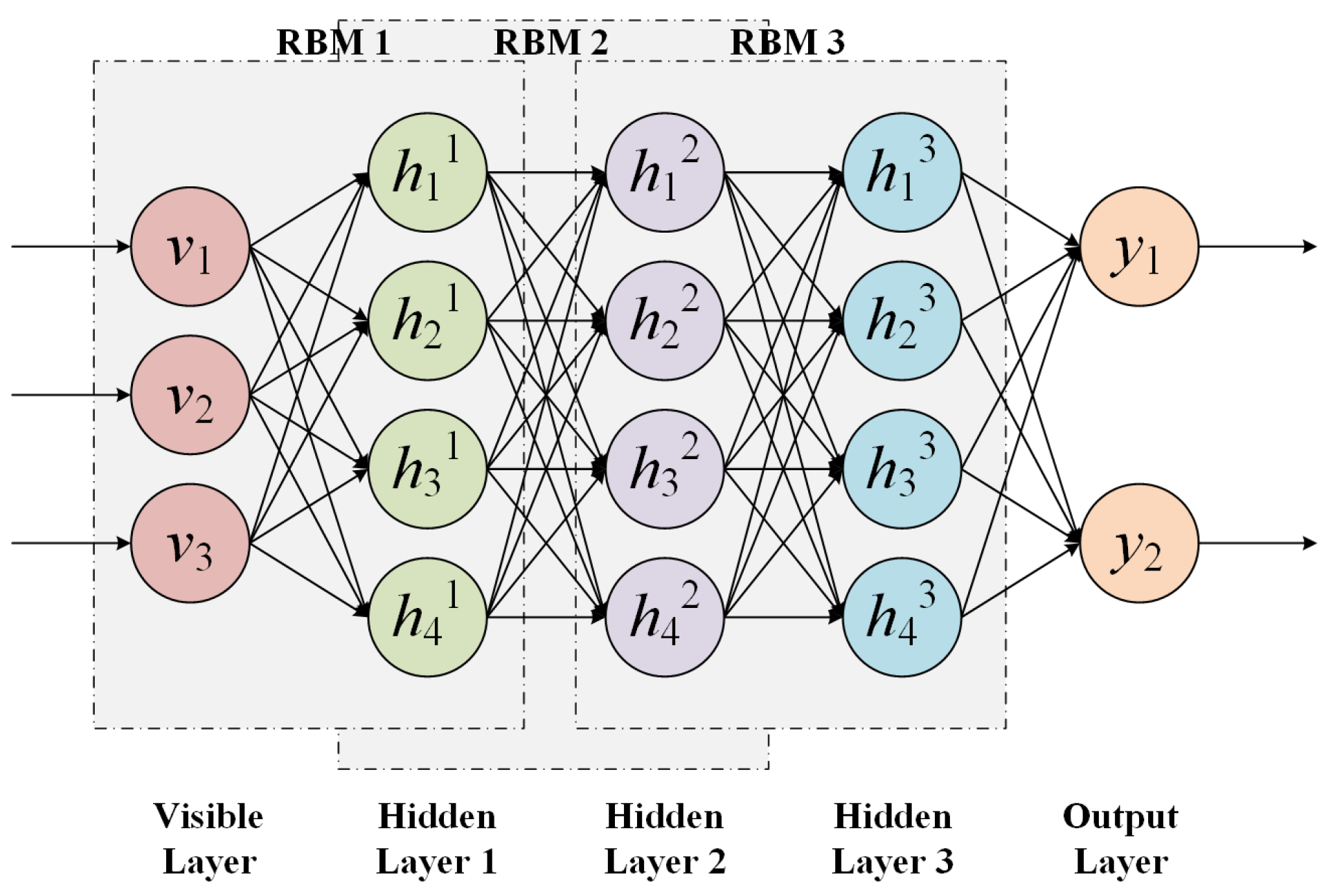
The deep belief network [24] is a deep neural network stacked by multiple RBMs. The DBN structure is shown in Figure 3. During the training process, the DBN first uses an unsupervised greedy layer-by-layer training algorithm for each layer of the RBM, except for the first and last layers of the DBN structure, where each layer of the RBM hidden layer serves as the visible layer of the next layer of the RBM, to transfer feature information and learning information (this phase is also called the pre-training phase of DBN). After the pre-training is completed, a small amount of labeled data are attached to the last layer of the DBN model, and supervised training is performed on each layer of the RBM. The backward propagation algorithm propagates the error information to each layer of the RBM and uses the maximum likelihood function for the objective function, which can optimize the whole DBN, thus obtaining the optimal low-dimensional representation of the original data.
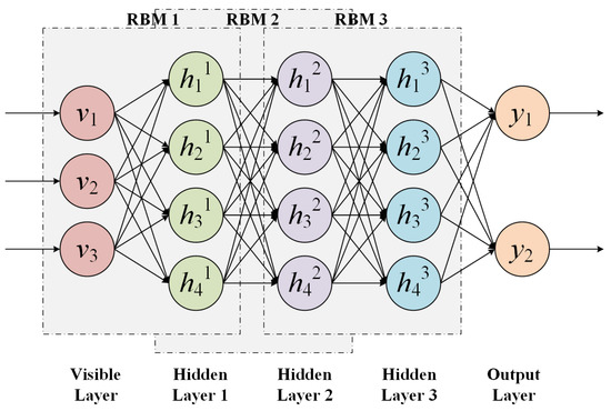
Figure 3.
The structure of DBN.
3.3. Broad Learning System
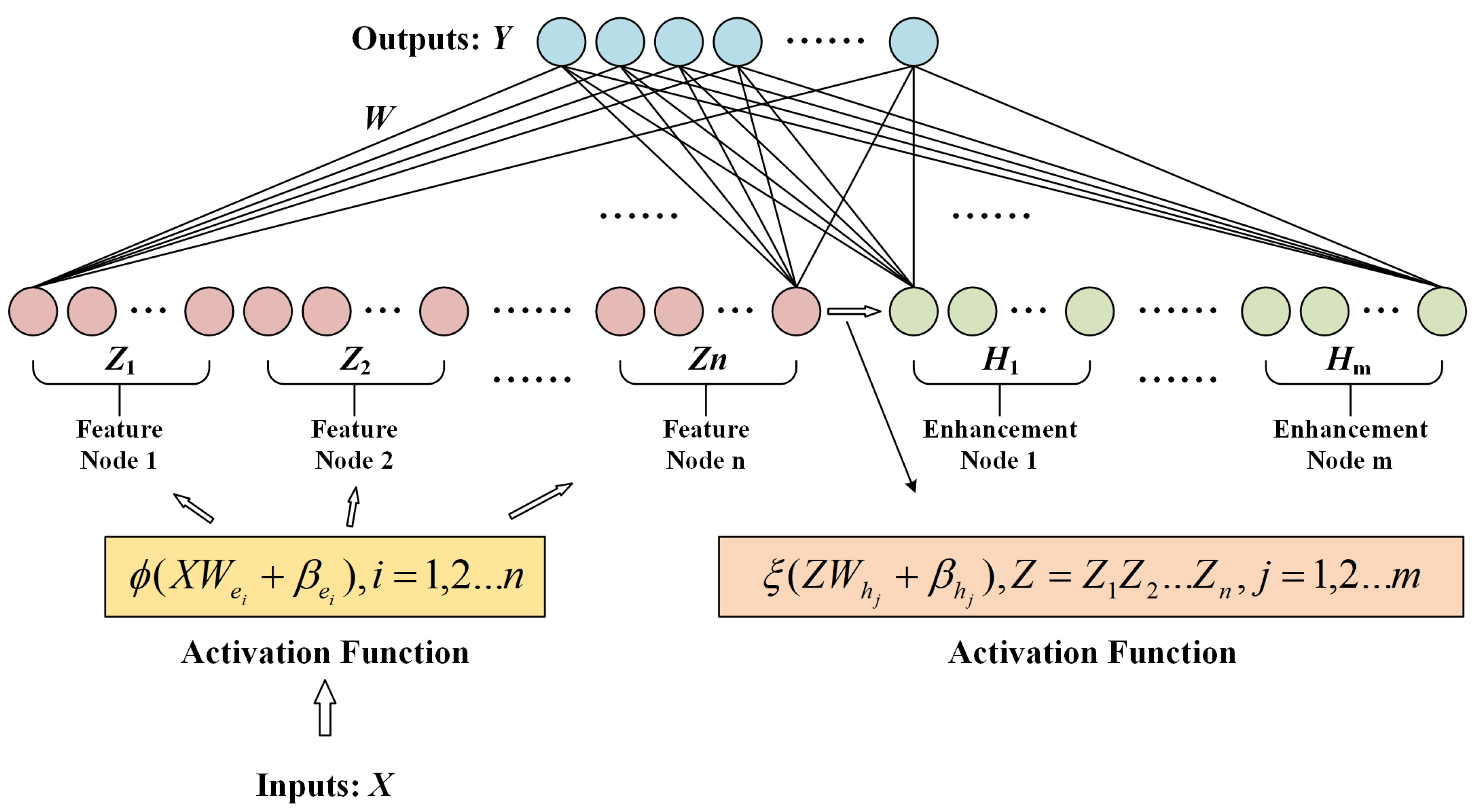
The carrier of a broad learning system [10] is a random vector function linked neural network. Compared with the deep learning method, the BLS has only two layers of neural network, and its structure is in the form of width extension. Its model structure is shown in Figure 4. Firstly, the BLS maps the input data into a feature node matrix through the mapping function. Secondly, the feature node matrix forms an enhancement node matrix by using the enhancement function. Then, the feature mapping nodes and the enhancement nodes are used together as the input of the hidden layer. Finally, the pseudo-inverse operation is used to calculate the weight matrix between the hidden layer and the output layer to achieve the purpose of training the BLS model.
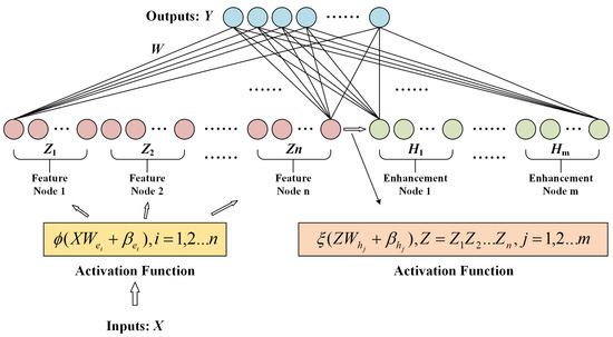
Figure 4.
The structure of BLS.
Suppose that the input data belong to and the output matrix, belongs to , where is the total data sample, is the sample dimension, is the number of categories of the data sample, is the feature node matrix, is the enhancement node matrix, and is the output weight matrix between the hidden layer and the output layer.
The specific procedure of the BLS is as follows. First, the sample data are mapped by group features to obtain the group feature node matrix , where :
where is the activation function, is the number of feature nodes corresponding to each feature mapping, is the weight matrix of the th feature mapping, and is the bias matrix of the th feature mapping. Both and are randomly generated. Then, all feature node matrices are integrated to obtain the total feature node matrix:
Second, the total feature node matrix undergoes group enhancement mapping to obtain the group enhancement node matrix , where , is as follows:
where is the activation function, represents the number of enhancement nodes corresponding to each group of enhancement transformations, is the group enhancement mapping weight matrix, and is the group enhancement mapping bias matrix. The total enhancement node matrix is obtained by integrating all enhancement node matrices:
Then, the feature mapping nodes are merged with the enhancement nodes as inputs to the BLS, defined as :
Finally, the predicted value of the broad learning algorithm can be given as
where is the weight matrix of feature nodes and enhancement nodes to the output layer.
To minimize the error between the predicted value and the true value and to find a suitable , the BLS model is optimized with the following function:
where the first term is used to control the minimization of the training error, the second term is used to prevent the model from overfitting, and the value denotes the further constraints on the sum of the squared weights; we take derivative of the above function and let it take the value of zero, obtaining as
where is the mapping and enhancement matrix, is a penalty factor, is an identity matrix, and is the true label.
3.4. Equalization Loss v2
The basic idea of equalization loss v2 [21] is to equalize the degree of learning of the model for different classes of samples by weighting the positive and negative gradients of each classifier according to the cumulative gradient ratios of the positive and negative gradients of the classifier, respectively. In solving the problem of imbalanced datasets, a classic strategy is the focal strategy, and Eqlv2 is improved on this basis. However, EQL v2 offers distinct advantages over focal loss, particularly in handling class imbalance without introducing bias towards minority classes. Unlike focal loss, which adjusts the loss contribution based on prediction difficulty, EQL v2 dynamically balances gradients during training, reducing overfitting on rare categories while maintaining focus on common classes. This approach enhances model stability and performance across varied datasets, providing a more nuanced response to imbalance challenges. The positive and negative gradients for the output of each classifier concerning the loss are
where is the total number of samples, is the probability that the th sample is predicted to be of class , and is the value of the One-Hot truthful labeling matrix in which the th sample is of class .
EQL v2 weights are updated by first defining as the ratio of the cumulative positive gradient to the negative gradient of task up to iteration . In this iteration, the weights of the positive gradient and the negative gradient can be computed as follows:
where is a mapping function as
The positive gradient and negative gradient are obtained and then they are applied to the positive and negative gradients of the current batch, respectively, and the reweighted gradient is
Finally, the ratio of the accumulated positive gradient to the negative gradient of the iteration update is computed and denoted as
EQL v2 chooses the gradient statistic as a measure of whether a task is in a balanced training state, balancing the model based on how easy or difficult each classification is for the model to train, rather than simply considering the number of its positive and negative samples. Introducing the idea of gradient-guided weighting to DBN and BLS helps the model to be trained with more attention to the features of minority classes of samples, thus making the model more comprehensive and balanced in evaluating each class of samples. The model adjusts the optimal weight contribution of the iteration based on the impact of different categories of samples on the performance of the classification.
3.5. Broad Equalization Learning System
The of the broad equalization learning system is solved as follows; based on the EQL v2 positive and negative gradients, the sample positive and negative gradients can be given as follows:
where is the feature matrix of the mapped and enhancement nodes, is the true label, and is the weight matrix.
The gradient function can be constructed from the positive and negative gradients as
where is the positive gradient factor and is the negative gradient factor. The smaller is, the greater the probability of positive samples, and the smaller the probability of negative samples. Adjusting the parameters and can adjust the learning effect of the model on different samples to achieve equalization of the degree of contribution of each class of samples to the model learning classification.
Based on the BLS loss function,
where is the penalty factor; then, the optimization objective of the BELS is the EQL v2 gradient function and the BLS loss function:
Among them, the first part is the loss function, which is used to control the classification error of the model. The second part is the penalty term, which mainly prevents the model from overfitting. The third part is the gradient term, which is used to balance the learning degree of different samples and alleviate the poor performance of the model in detecting samples of minority classes.
The existing is expressed as by taking the partial derivative of :
where is a matrix with all elements equal to 1, is a positive gradient factor, is a negative gradient factor, the positive and negative gradient factors are used to control the learning degree of the model on different samples, and is a penalty factor to avoid the overfitting of the model caused by the excessively large .
4. Experiments
This section presents the detailed experiments. We analyze in detail the effect of hyperparameters on the model. We employ grid search to fix the positive and negative gradient factors within appropriate ranges, seeking the optimal parameter combination that maximizes the detection performance of the model. To evaluate the effectiveness of the proposed method, we conduct complete ablation experiments. Finally, we give a comparative analysis of the proposed model with other state-of-the-art methods.
4.1. CICIDS2017 Datasets
The CICIDS2017 dataset [25] proposed by the Canadian institute for cybersecurity is one of the important benchmark datasets for evaluating intrusion detection models. The authors used the behavior profile system to analyze the abstract behavior of human interactions based on different protocols, constructing 25 abstract behaviors of users and generating natural friendly background traffic. The dataset contains benign and new common attacks and includes seven types of network attacks, namely denial-of-service attacks, secure shell brute force attacks, botnet attacks, distributed denial-of-service attacks, web application attacks, heartbleed exploits, and penetration testing attacks. The sample distribution and features of the dataset are shown in Table 1.

Table 1.
Class distribution of CICIDS2017 dataset.
4.2. Implementation Details
The DBELS model parameters were set as in Table 2, including the training parameters of the DBN dimensionality reduction model, the BELS activation function, the number of nodes in each of the mapping groups, the number of nodes in each of the enhancement groups, and the penalty coefficient, . The DBN dimensionality reduction model consisted of a stack of three RBMs, (49,64), (64,32), and (32,16). All the experiments were conducted using a 64-bit Intel(R) Core (TM) i7-11700 CPU with 32 GB RAM in the Windows 11 environment. The models were implemented in Python v3.9.16 using the PyTorch v2.1.0 library.
Table 2.
The parameters of DBELS.
4.3. Performance Metrics
The evaluation metrics for intrusion detection mainly include accuracy, recall, and false positive rate (). In the formula, the true positive () represents the number of samples correctly identified as positive, the true negative () is the number of samples correctly identified as negative, the false positive () is the number of negative samples incorrectly identified as positive, and the false negative () is the number of positive samples incorrectly identified as negative. The denotes the ratio of the number of samples correctly classified by the model to the total number of samples:
The denotes the proportion of positive cases in the sample that are correctly predicted, also known as the detection rate:
The false positive rate is the proportion of truly negative samples that the model incorrectly classifies as positive:
4.4. Analysis of Hyperparameters
4.4.1. Effect of and on Binary Classification
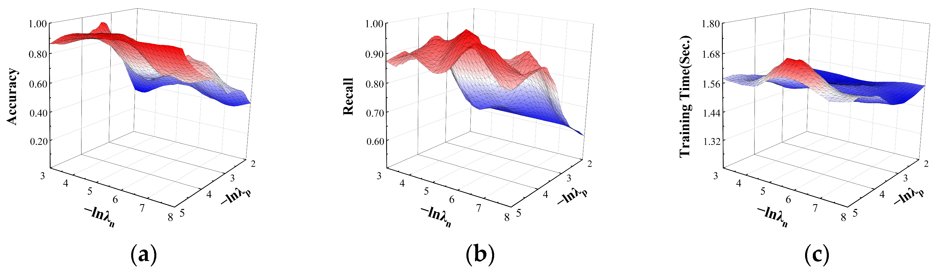
For the two parameters and in the DBELS model, their effects on the performance of the model in different classification tasks were explored. Their effects on the performance of accuracy, recall, and time in the binary classification task are shown in Figure 5. For accuracy and recall, the performance tends to increase with decreasing and . Different parameter combinations lead to larger differences because the model is more sensitive to the two parameters in the binary classification task, and as the order of magnitude improves, the performance of the model changes drastically. The experiments show that when is around orders of magnitude and is around orders of magnitude, the model can maintain higher accuracy and recall, at around 0.99 and 0.98, respectively. For the training time of the model with the change in and , the training time fluctuates slightly above and below 1.6 s, indicating that the model training time in the binary classification task is not sensitive to the positive and negative factors.
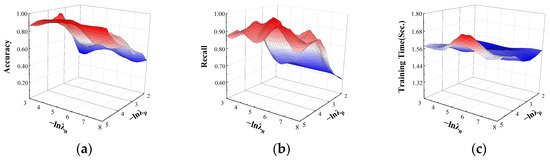
Figure 5.
The effect of and on binary classification. The effects on the performance: (a) the effect on accuracy; (b) the effect on recall; (c) the effect on training time.
4.4.2. Effect of and on Multi-Classification
In the multi-classification task, its effect on the accuracy, recall, and time performance are shown in Figure 6. For accuracy, the model is almost insensitive to and almost tends to be stable as changes; when , the accuracy increases as increases. For recall, as and increase, the recall of the model tends to increase. When the value’s order of magnitude is and the value’s order of magnitude is about , recall grows to a maximum of about 0.95. For the model training time with the change in and , the time of the model fluctuates from 1.4 s to 1.6 s and almost stabilizes, which shows that the training time is not sensitive to the positive and negative factor parameters. To achieve a better overall performance, the order of magnitude of is around , and the order of magnitude of is around , which can make the accuracy stabilize to 0.96 and the recall stabilize to 0.95.
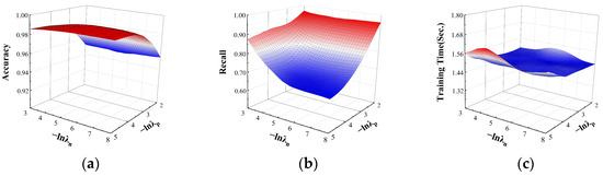
Figure 6.
The effect of and on multi-classification. The effects on the performance: (a) the effect on accuracy; (b) the effect on recall; (c) the effect on training time.
4.4.3. Effect of Mapping and Enhancement Groups on Binary Classification
The experiments explored the effects of DBELS model enhancement groups and mapping groups on the performance of the model for different classification tasks. For the binary classification task, the effects of enhancement groups and mapping groups on accuracy, recall, and training time are shown in Figure 7. For accuracy and recall, the model floats more with the change in parameters because the binary classification task model is more sensitive to these two parameters. With the increase in the mapping matrix and the enhancement matrix , its input matrix increases, and the model detection performance is highly dependent on the matrix, . For training time, it increases with the increase in enhancement groups and mapping groups, because the input matrix increases with the increase in parameters. From the experimental results, it is known that when enhancement groups and mapping groups are selected as 1, it can ensure both less training time and higher accuracy and recall.
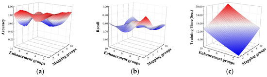
Figure 7.
The effect of enhancement groups and mapping groups on binary classification. The effects on the performance: (a) the effect on accuracy; (b) the effect on recall; (c) the effect on training time.
4.4.4. Effect of Mapping and Enhancement Groups on Multi-Classification
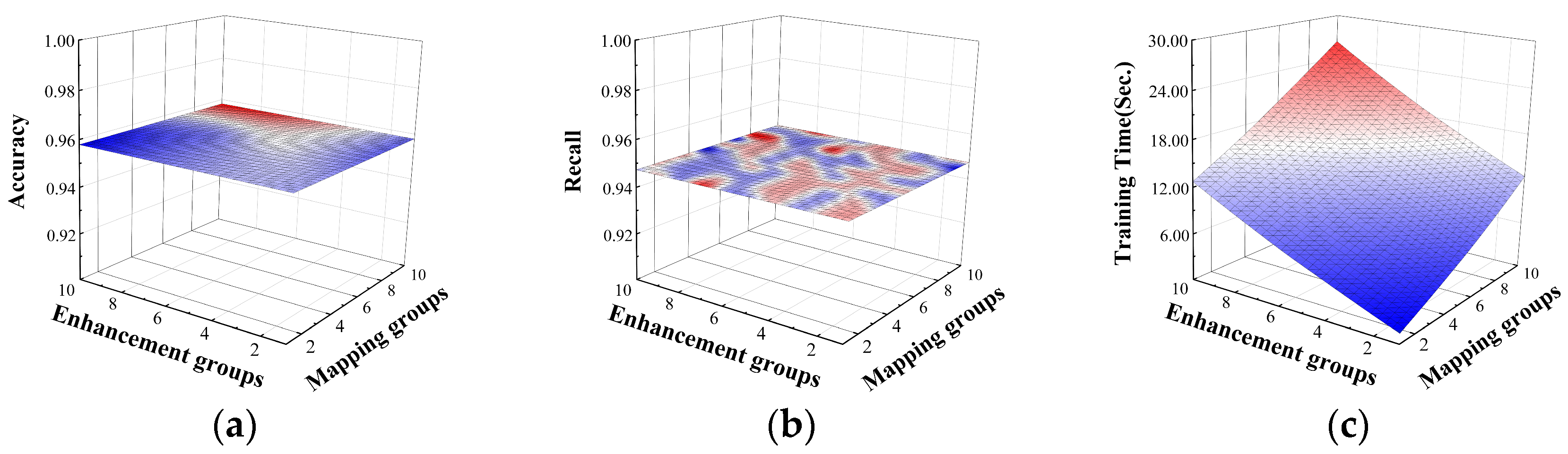
For the multi-classification task, the effects on accuracy and recall are shown in Figure 8. With the increase in enhancement groups and mapping groups, the accuracy and recall almost tend to stabilize, indicating that for the multi-classification task, these two metrics of the DBELS model are not sensitive to the mapping and enhancement groups. The training time shows an upward trend in time consumption both with the increase in mapping groups and enhancement groups. The reason is that the increase in mapping groups and enhancement groups increases the size of the mapping matrix and the enhancement matrix , resulting in an increase in matrix , increasing the burden on and consumption of the model. It can be concluded that since the increase in enhancement groups and mapping groups has less impact on the detection performance of the model and increases the consumption of time cost when enhancement groups and mapping groups are selected as 1, the accuracy and recall maintain a higher performance and the time consumption is minimized.

Figure 8.
The effect of enhancement groups and mapping groups on multi-classification. The effects on the performance: (a) the effect on accuracy; (b) the effect on recall; (c) the effect on training time.
4.5. Ablation Studies
To evaluate the effectiveness of the proposed method, we performed ablation experiments based on three dimensionality reduction models and two classification models. The three dimensionality reduction models are traditional PCA, traditional DBN, and DeBN with the introduction of EQL v2. The classification methods are traditional BLS and our improved BELS, respectively. We evaluated the detection performance of a total of eight methods under a binary classification task and multi-classification task based on the CICIDS2017 dataset. All the experiments were conducted in the same environment with identical forms of data processing, and the detection performances of different models are shown in Table 3 and Table 4. The recognition rate of each sample under different classification tasks is shown in Table 5 and Table 6.
Table 3.
The performance of different methods on binary classification.
Table 4.
The performance of different methods on multi-classification.
Table 5.
The recall of each sample on binary classification.
Table 6.
The recall of each sample on multi-classification.
4.5.1. Performance Analysis on Binary Classification
In the binary classification task, the traditional BLS structure is less effective in recognizing the CICIDS2017 dataset, mainly due to the high-dimensional redundant information in the dataset that affects the classification performance, resulting in lower accuracy and recall, especially the lack of attention to the minority-class samples in the imbalanced dataset. After the introduction of EQL v2, the accuracy and recall of the BELS model significantly improved, indicating that EQL v2 enhances the ability to recognize minority-class samples in dealing with the imbalance problem. The deep belief network broad learning system (DBLS) model reduces the data redundancy through the DBN dimensionality reduction, which improves the accuracy and recall, which were improved by 0.034 and 0.106, respectively. The DeBLS model overly focuses on minority-class samples during DeBN dimensionality reduction, resulting in a decrease in the detection performance for majority-class samples.
DBELS has the highest detection performance in the binary classification task, and the introduction of EQL v2 on top of the DBLS improves the accuracy and recall by 0.077 and 0.249, respectively, indicating that the combination of DBN dimensionality reduction and EQL v2 significantly improves the model performance. Although the DeBELS model introduces EQL v2 to the DeBN dimensionality reduction dataset and improves the model performance by adjusting the parameters of positive and negative gradient factors, the accuracy and recall slightly decreased by 0.004 and 0.01, respectively, compared with DBELS, which reflects the negative impact of overlearning abnormal samples on classification performance. For the principal component analysis broad learning system (PBLS) model, after the PCA dimensionality reduction, accuracy and recall decreased by 0.014 and 0.040, respectively, compared with the BLS, mainly due to more information loss during PCA dimensionality reduction and the inability to deal with imbalanced datasets efficiently. The principal component analysis broad equalization learning system (PBELS) model had an accuracy of 0.923 and a recall of 0.853, compared with PBLS, with an improvement of 0.055 and 0.262, indicating that EQL v2 can still significantly improve the detection performance of minority-class samples even when PCA dimensionality reduction is ineffective. However, the PBELS reduced accuracy and recall by 0.070 and 0.106, respectively, compared with DBELS, further demonstrating that DBN dimensionality reduction outperforms PCA dimensionality reduction in binary classification tasks.
4.5.2. Performance Analysis on Multi-Classification
In the multi-classification task, the traditional BLS performed poorly, with an accuracy of 0.975 and a recall of only 0.474, mainly due to the severe imbalance of the dataset that affects the classification performance. The BELS model after the introduction of EQL v2 had an improved recall of 0.051, mainly because EQL v2 improves the data imbalance problem, which allows the model to increase the weight of the attack samples for minority classes and thus improves the detection rate. The DBLS model, after dimensionality reduction by DBN, had an improved accuracy of 0.018 and an improved recall of 0.184, which is attributed to the fact that the DBN dimensionality reduction reduces the data redundancy, mitigates the negative impact of raw data, and improves the detection performance of the model. The DeBLS model improved recall by 0.02 compared with DBLS, which is attributed to the fact that DeBN learns more about the minority-class samples, eliminates redundancy between different samples, and at the same time retains the key features of the minority-class samples, which improves the classification and detection performance. The DBELS model improved by 0.018 in DBN dimensionality reduction, and with the introduction of EQL v2, accuracy improved by 0.017 and recall improved by 0.278; compared with DBLS, recall improved from 0.658 to 0.803, which is attributed to the fact that EQL v2 balances the learning weight of the minority-class samples and increases the focus on the minority-class samples.
The accuracy for the DeBELS model of 0.957 and recall of 0.947 was the best performance in the multi-classification task, and recall was significantly improved by 0.27 compared with DeBLS, which is because the improved BLS model is better able to deal with unbalanced datasets and enhances the ability to recognize minority-class attacks. The recall of DeBELS improved by 0.144 compared with DBELS, and the overall classification performance improved significantly. The accuracy of the PBLS model decreased by 0.037 and the recall decreased by 0.176 after PCA dimensionality reduction, since PCA dimensionality reduction leads to more loss of information, which affects the multi-classification effect. The accuracy of the PBELS model was 0.938 and recall was 0.470; compared with PBLS, accuracy and recall were improved by 0.001 and 0.173, respectively, indicating that the introduction of EQL v2 improves the detection rate of minority-class samples. However, compared with DeBELS, the accuracy and recall of PBELS were reduced by 0.019 and 0.477, respectively, which indicates that DBN dimensionality reduction is much better than the PCA dimensionality reduction model in terms of detection performance, and once again proves the superiority of the proposed model in multi-classification tasks.
4.5.3. Time-Cost Analysis
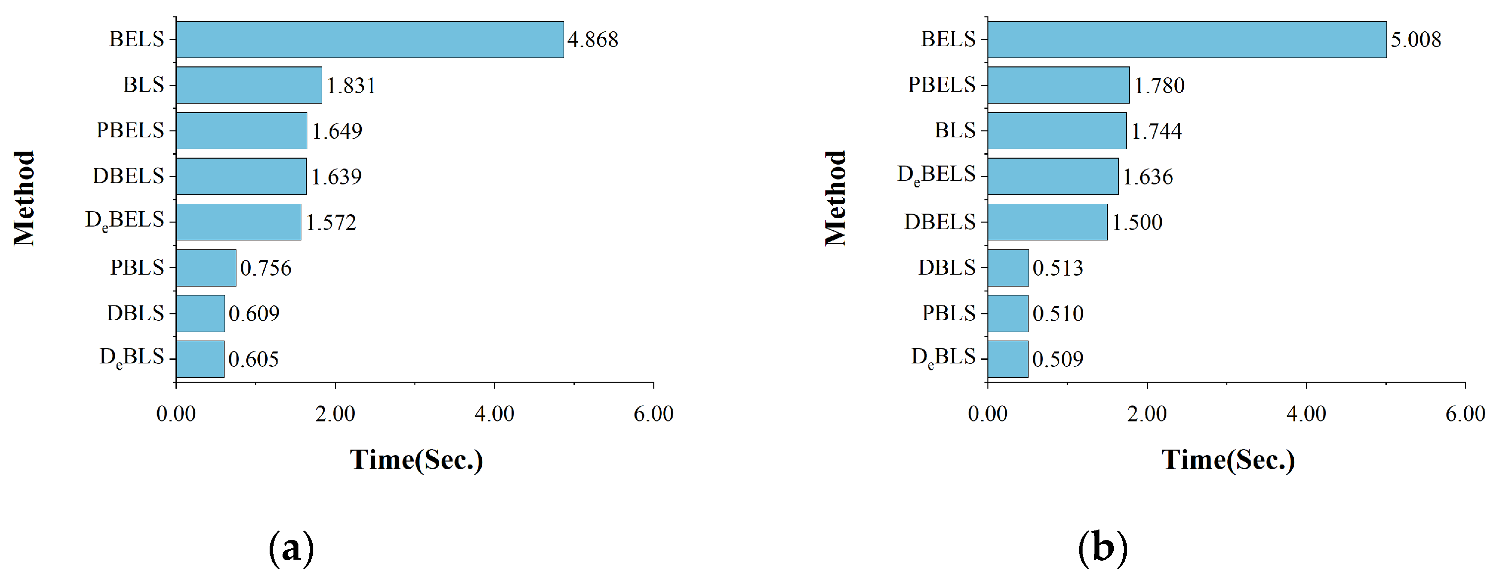
The comparison of the training times for the different models is shown in Figure 9. For binary classification and multi-classification, the training time of the traditional BLS was about 1.8 s, reflecting the advantage of shallow networks with lower time costs in model classification. The training time of BELS was about 5 s, and the time increase was because the introduction of EQL v2 requires the additional performance of multiple matrix operations. The training time of the DBLS model was about 0.5 s, which is a significant reduction compared with the BLS model, indicating that the high-dimensional data have a significant negative effect on the model training time, and the reduced dimensionality of the dataset reduces the training time to 25% of the original one. The training time of DeBLS was also about 0.5 s, which indicates that the introduction of EQL v2 after the dimensionality reduction of DBN has almost no effect on the training time.
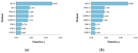
Figure 9.
The comparison of training time for different methods: (a) binary classification; (b) multi-classification.
The training time for DBELS was about 1.5 s, which is greatly reduced compared with BELS, thanks to the dimensionality reduction of the DBN model for high-dimensional data. However, there was an increase compared with DBLS due to some additional computations required by the improved BELS model. The training time of DeBELS was about 1.6 s, which is almost the same as that of DBELS, indicating that the introduction of the low-dimensional dataset with EQL v2 does not have a significant impact on the training time, and there is a slight increase in the cost of time due to a small number of additional computations of the positive and negative gradient matrices in comparison with DeBLS.
The results show that the hybrid DBN and BLS-based models DBELS and DeBELS maintained low time consumption compared with the traditional BLS models, following the advantages of the shallow BLS networks that are computationally fast and easy to train. Although the PCA dimensionality reduction model also reduces some of the training time, its detection performance is greatly degraded, again confirming the advantages of the DBN-based dimensionality reduction model. The proposed model is comparable with the traditional deep learning model, which has a significant advantage in time cost consumption, which is conducive to saving a certain amount of computational resources in practical applications.
4.5.4. Results Analysis for Recall of Each Sample on Binary Classification
The detection rate of Benign and Attack samples under the binary classification task is shown in Table 5. The traditional BLS performed poorly in detecting Attack samples with a recall of only 0.261, which is due to the overlearning of the majority-class samples when dealing with imbalanced datasets, resulting in a low detection rate for minority-class samples. With the introduction of the BELS model with EQL v2, the detection rate of Attack significantly improved to 0.863, which significantly improves the identification of minority-class samples. The DBLS model with DBN dimensionality reduction improved the detection rate of Attack by 0.213, which suggests that DBN dimensionality reduction reduces the data redundancy and has a positive impact on the subsequent model classification. In the DeBLS model, the detection rate of Attack was as high as 0.996, but the detection rate of Benign was only 0.165, which shows that DeBN dimensionality reduction focuses excessively on minority classes of samples, resulting in a decrease in the recognition performance of the majority of classes of samples.
The DBELS model, after dimensionality reduction by the introduction of EQL v2, had a detection rate of 0.996 for Benign and 0.976 for Attack, which improved the detection rate of the two classes of samples by 0.009 and 0.113, respectively, compared with the BELS model. Because DBN dimensionality reduction reduces the redundant features and improves the classification performance of the model, compared with DBLS, DBELS significantly improved the detection rate of Attack from 0.474 to 0.955, which is attributed to the fact that EQL v2 balances the sample weights so that the model focuses on each class of samples in a more balanced way. The detection rates of Benign and Attack for the DeBELS model were 0.995 and 0.955, respectively, and compared with DeBLS, the Benign detection rate was substantially higher and the Attack detection rate was slightly lower, but EQL v2 improved the detection performance by making the model more balanced in focusing on each class of samples. Compared with DBELS, the detection rate of Benign for DeBELS was almost unchanged, and the detection rate of Attack slightly decreased, which is attributed to the overlearning of minority-class samples brought by DeBN, but the classification still performed well through the adjustment of positive and negative gradient factors.
The detection rate of Attack for the PBLS model was only 0.182 after the PCA dimensionality reduction, which is a decrease from that of the BLS model of 0.080. PCA dimensionality reduction leads to information loss, which negatively affects the classification detection effect of minority-class samples. The Attack detection rate of the PBELS model was 0.749, which improved by 0.567 compared with the PBLS. The introduction of EQL v2 makes the model focus on each class of sample in a more balanced way, which improves the detection performance of the minority-class samples. Despite the improvement of the PBELS model, its Attack detection rate was still 0.227 lower than that of DBELS, which further proves the superiority of the DBN dimensionality reduction model in detection performance.
4.5.5. Result Analysis for Recall of Each Sample on Multi-Classification
The detection rates of different methods for each type of sample under the multi-classification task are shown in Table 6. The traditional BLS did not work well when dealing with the unbalanced CICIDS2017 dataset, and although it had better detection performance for a larger number of samples (e.g., Benign, DoS/DDoS, Port Scan), it was poor in detecting samples of a few classes (e.g., Botnet ARES, Brute Force, Web Attack). This is because the BLS model is unable to balance the contributions of various classes of samples when dealing with unbalanced datasets, resulting in a very low detection rate for minority-class samples. The introduction of the BELS model with EQL v2 significantly improved the detection rate of Brute Force attacks, which in turn improved Attack identification. However, Botnet ARES and Web Attack were still undetectable because the features of these minority-class samples are highly similar to other samples, which the model is unable to differentiate, leading to false positives. The DBLS model eliminates certain data redundancies after dimensionality reduction by DBN, which enhances the detection performance. The detection rate of Brute Force was improved to 0.985, but Botnet ARES and Web Attack were still not detected. This indicates that dimensionality reduction alone cannot solve the problem of unbalanced datasets, especially for classes with a very small number of samples.
The DeBLS model further improved the detection performance, and most of the attack types were detected, including Botnet ARES. This is because DeBN dimensionality reduction learns more about the minority-class samples and preserves their key features, but Web Attack was still undetectable, which requires further focus on the minority-class samples. The DBELS model showed a significant improvement in the detection rate of most attack types compared with BELS and DBLS, especially Web Attack, from 0 to 0.856. This is because DBN dimensionality reduction reduces the data redundancy, while EQL v2 makes the model focus better on the minority-class samples. However, Botnet ARES was still not detected, which suggests that DBN dimensionality reduction is not enough to solve the problem. The DeBELS model maintained a high detection rate on all attack types. Compared with DeBELS, the detection rate of Botnet ARES improved from 0.137 to 0.948, and Web Attack improved from 0 to 0.856. This is because the introduction of EQL v2 improves the ability to better recognize and learn the minority-class samples, which significantly improves the detection rate. DeBELS further improved the detection rate of Botnet ARES compared with DBELS because DeBN dimensionality reduction preserves the key features of the minority-class samples at a finer granularity and mitigates the data imbalance problem.
The PBLS model using PCA dimensionality reduction only detected the highest number of DoS/DDoS attacks, while Port Scan, Botnet ARES, Brute Force, Web Attack, and other attacks were not detected. Compared with the BLS model, Port Scan could not be detected due to the loss of information caused by PCA dimensionality reduction, which affects the multi-classification effect. After the introduction of EQL v2 to the PBELS model, the detection rate of Port Scan improved to 0.978, but the other few classes of attacks (e.g., Botnet ARES, Brute Force, and Web Attack) still went undetected. This suggests that PCA dimensionality reduction leads to the loss of key features. Compared with DeBELS, the detection performance of PBELS was worse, which indicates that DBN-based dimensionality reduction outperforms traditional PCA dimensionality reduction in terms of detection performance.
4.6. Analysis of ROC-AUC
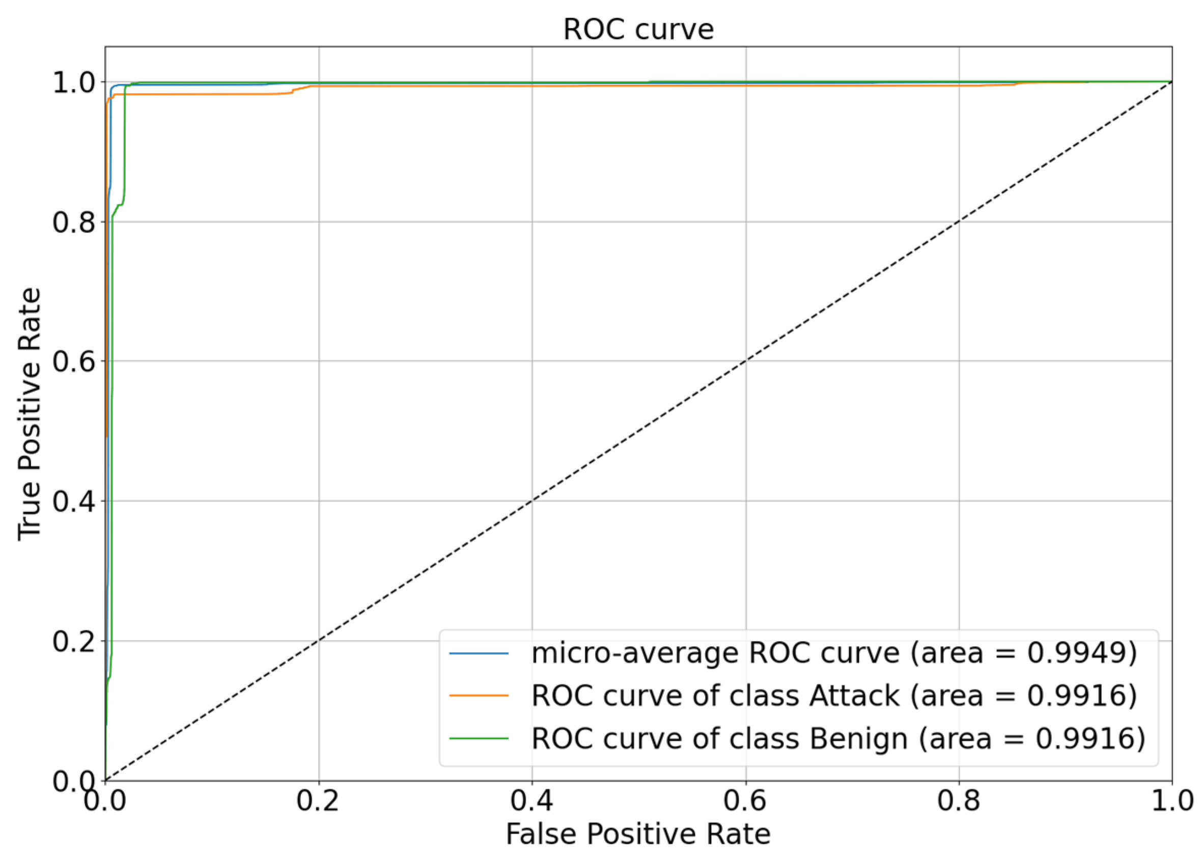
Figure 10 shows the receiver operating characteristic (ROC) curves for the DBELS binary classification. The overall average ROC curve has an area under the curve (AUC) of 0.9949, indicating that the DBELS classifier performed excellently on the entire dataset and is close to being a perfect classifier. Secondly, the ROC curves for the two categories (Attack and Benign) can be observed, each of them with an AUC of 0.9916, which indicates that the classifier also had high performance when considering each category individually, especially when dealing with a minority number of samples. The AUC close to 1 implies that the classifier has a very high true positive rate (TPR) in its predictions for the category while maintaining a relatively low FPR. This means identifying as many true positive samples as possible while keeping the misdiagnosis rate as low as possible. Taken together, the DBELS classifier had excellent performance on the entire imbalance dataset for both minority-class samples and majority-class samples.
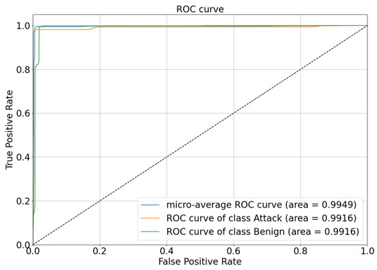
Figure 10.
The ROC of DBELS on binary classification.
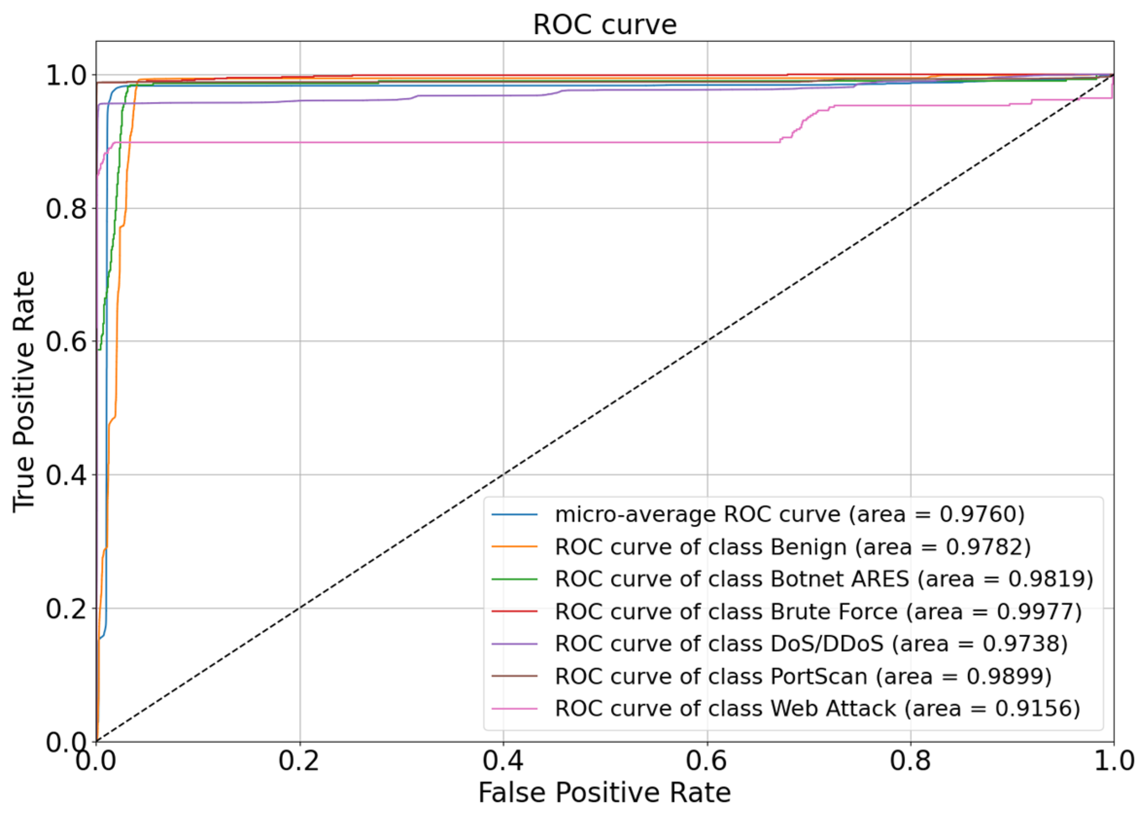
The DeBELS multi-classification ROC curve is shown in Figure 11. The overall average ROC curve has an AUC of 0.9760, which indicates that the classifier performed well on the whole dataset. The Benign, Botnet ARES, Brute Force, DoS/DDoS, and Port Scan detections performed well; their AUC areas were all more than 0.9700, although Web Attack had the lowest AUC area of 0.9100, but it is already better than other models at the same level. Overall, after the introduction of the EQL v2 positive and negative gradient factors, by adjusting the parameter weights, the model can pay more attention to minority classes of samples in the face of imbalanced datasets, thus improving detection performance.
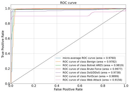
Figure 11.
The ROC of DeBELS on multi-classification.
4.7. Comparison with State-of-the-Art Methods
4.7.1. Binary Classification
The false alarm rate and time cost of all the algorithms were compared on the binary classification task, as shown in Figure 12. For FPR, the proposed model had a lower false alarm rate of 0.014, which was better than the other models. This indicates that the proposed model incorrectly labels normal situations as abnormal less often and correctly identifies and classifies normal situations more often, as compared with other methods. For the model training time, the proposed model required less training time and detection time in the binary classification task, with a time consumption of around 1 s. The time cost of the model is much lower than the deep learning model and has an advantage over other machine learning algorithms, which can significantly reduce the time cost and ensure faster training of the model for large-scale datasets.
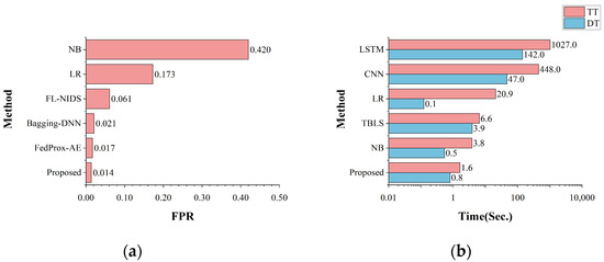
Figure 12.
The comparison with state-of-the-art methods on binary classification: (a) the comparison of FPR; (b) the comparison of time cost.
The binary classification detection performance of the different models of recent years is given in Table 7. The proposed model had higher accuracy, recall, and lower FPR in binary classification, which indicates that the proposed model can detect normal and abnormal behaviors well. Compared with traditional machine learning models, the proposed model outperforms the logistic regression (LR) and naive bayes (NB) in accuracy, recall, and FPR. Compared with other BLS-based models, accuracy and recall are better than TBLS. Compared with deep learning models, the proposed model outperforms most of the models, and the performances of the fusion of statistical deep neural network (FS-DNNs) and multi-objective evolutionary convolutional neural network (MECNN) are slightly higher than the proposed model; however, since both models are based on deep learning models, their model size and training time cost are much higher than the BLS-based model. Considering the bagging ensemble learning deep neural network (Bagging-DNN) model, its accuracy is lower than the proposed model, and its recall is slightly higher than the proposed model, but in addition to the higher space and time complexity brought by its deep learning model, the false alarm rate is also higher than the proposed model. In summary, the proposed model has better detection performance and a lower false alarm rate in binary classification and has obvious advantages over the other models.
Table 7.
The comparison with state-of-the-art methods of binary classification.
4.7.2. Multi-Classification
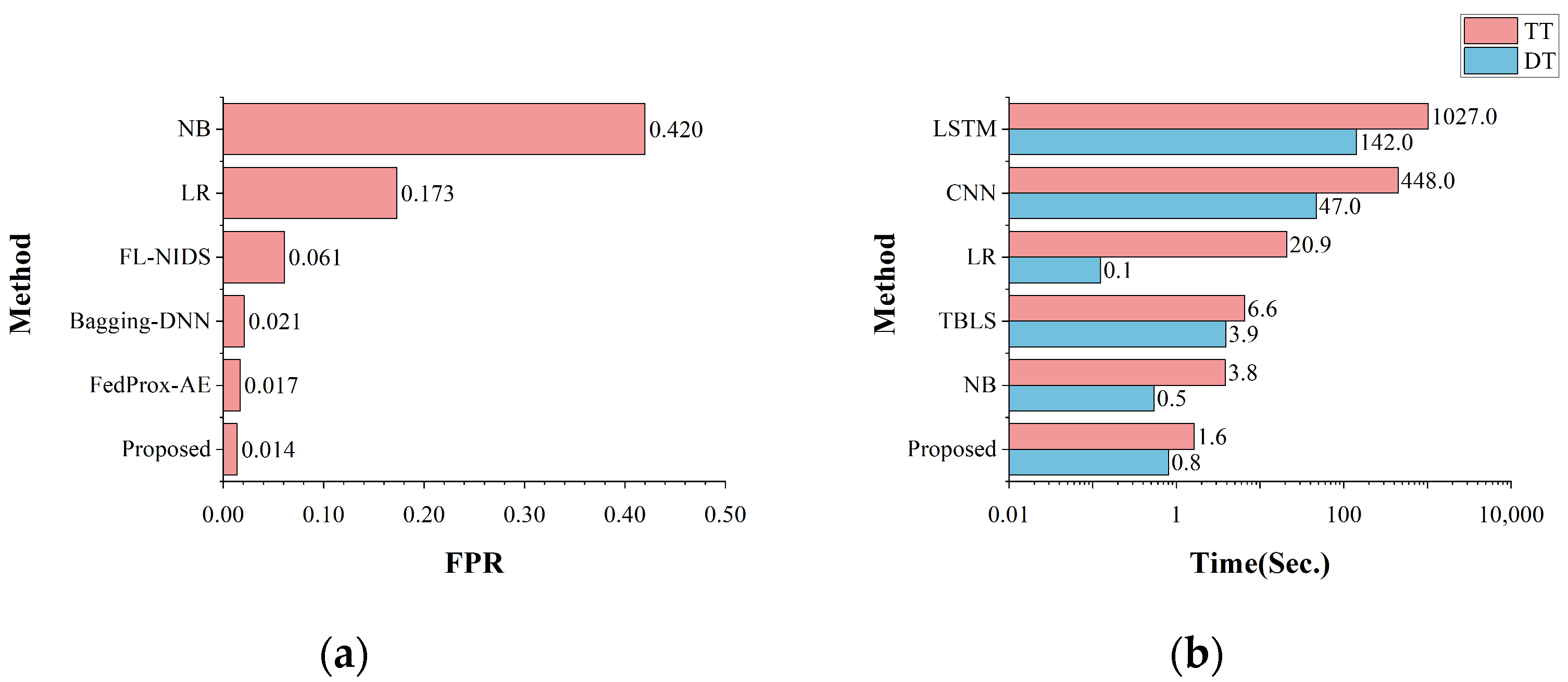
The false positive rate and time cost of all the other algorithms on the multi-classification task are shown in Figure 13. The FPR graphs show that the proposed model had only a 0.012 false positive rate, which is lower than the other models. This means that the model can recognize different categories of attacks better and misclassify less often during the multi-classification task and perform the task of detecting and identifying attack samples better. The model required less training time and detection time compared with other models, offering advantages in handling large-scale data and enhancing its suitability for real-world dataset environments.
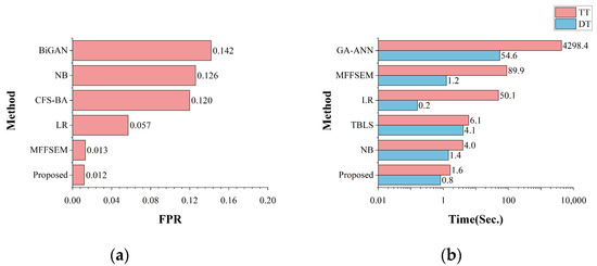
Figure 13.
The comparison with state-of-the-art methods on multi-classification: (a) the comparison of FPR; (b) the comparison of time cost.
The multi-classification detection performance of different models in recent years is given in Table 8. The proposed model has higher accuracy and recall and lower FPR under multi-classification task, which indicates that the proposed model can detect both normal and abnormal behaviors well and detect each specific class of attacks better. Comparing the traditional machine learning algorithms, we see that the proposed model outperforms LR and NB in terms of accuracy, recall, and FPR. Compared with other BLS models, the TBLS(W) model has a slightly higher accuracy and recall than the proposed model, since, for the TBLS, the authors only selected the dataset of a single day, Wednesday, for model training and testing. It only accounts for 30% of the total dataset, and the attack types are all DoS/DDoS type attacks, which are better balanced compared with the total dataset, and the detection performance of the model will be affected to some extent.
Table 8.
The comparison with state-of-the-art methods on multi-classification.
Compared with the other machine learning algorithms, for the multi-dimensional feature fusion and stacking ensemble mechanism (MFFSEM) and correlation-based feature selection bat algorithm (CFS-BA) models, the detection performances are better than that of the proposed model, but their FPRs are higher than the proposed model, which will lead to them overly misjudging normal behavior as an attack. The two models are also trained with the same dataset of only one day, Wednesday. Compared with the long short-term memory (LSTM) model, its accuracy is slightly higher than the proposed model, but its recall is much lower than the proposed model, which means that the LSTM model fails to recognize the attacks well. In summary, compared with other models, the proposed model has advantages such as better detection performance and a lower false alarm rate when performing the multi-classification task.
5. Model Validation
Network traffic in real environments is large and complex; to evaluate the DBELS model better and simulate the effect of real environments, we selected the CICIDS2018 dataset to test and validate the model’s performance in different data environments. The CICIDS2018 dataset is a widely used dataset in cybersecurity research and was created by the Canadian institute for cybersecurity research, which simulates real-world network traffic, including normal traffic and many types of attacks. Compared to the CICIDS2017 dataset, its size has increased by about four times and contains more than eight million traffic records; however, it also has a serious data imbalance. The dataset contains over eight million traffic records with up to 80 features per sample. These data cover both normal traffic and a wide range of attack traffic, with sample types mainly including Benign, DoS/DDoS, Brute Force, Botnet and Infiltration. The diversity and complexity of the sample types in the CICIDS 2018 dataset make the dataset a better reflection of real-world cyber threats, which makes it possible to comprehensively evaluate the performance and generalization capabilities of intrusion detection systems.
The model validation experiments using the CICIDS2018 dataset included data preprocessing and data dimensionality reduction, and the form of the operations remained consistent with CICIDS2017. The models for their comparison experiments include BLS, DT, NB, MLP, and CNN. To ensure the validity of the experiments, the data preprocessing is the same, and all the experiments are conducted in a consent environment. The evaluation metrics for the comparison experiment included accuracy, recall, false positive rate, and training time. The performance of different models under the binary classification task is shown in Table 9, and the performance under the multiple classification task is shown in Table 10.
Table 9.
The performance of different methods on binary classification for the CICIDS2018 dataset.
Table 10.
The performance of different methods on multi-classification for the CICIDS2018 dataset.
The results show that our proposed model outperforms most other models in accuracy, recall, FPR and time cost under different classification tasks. For the binary classification task, compared to the traditional BLS structure, accuracy and recall are improved by 0.023 and 0.025, respectively, and the false alarm rate is decreased by 0.025. Compared to the traditional machine learning algorithms DT and NB, both of them have a significant improvement in the detection performance, while the false alarm rate is decreased significantly. For the deep learning algorithms MLP and CNN, the detection performance is improved and the model training time is reduced significantly. For the multi-classification task, the proposed model also maintains high detection performance and low model training time, and compared to the NB model, it has a significant advantage in detection performance, although the model training time is slightly improved. Compared with the CNN model, although the accuracy slightly decreases by 0.02, it is better than the CNN model in terms of recall, FPR, and model training time.
From the above experimental results, it can be concluded that the proposed model can still show better detection performance when facing the CICIDS2018 dataset with a larger and more complex scale, which further indicates that the model has a certain degree of scalability and adaptability. The scale of this dataset is greatly increased compared to the CICIDS2017 dataset; however, the proposed model can still maintain low time consumption, which further verifies that the model has a certain degree of adaptability and lightness for real complex environments. Our proposed model consistently demonstrates strong detection performance and low time consumption across various datasets, whether for binary or multi-class classification. This efficiency is crucial for real-world applications, where maintaining high accuracy and speed is essential. Additionally, the model’s adaptability to different data environments and robustness against diverse threats enhances its practical value. Its scalability ensures it can handle increasing data volumes, making it a versatile solution in dynamic cybersecurity landscapes.
6. Conclusions
In this paper, based on the BLS model and introducing the EQL v2 reweighting idea, we propose a DBELS model, which aims to solve the problem of the traditional BLS facing low detection rates for high-dimensional and imbalanced datasets in the field of NIDSs, as well as the low recognition of minority-class attacks. First, the model fully learns the large-scale high-dimensional dataset through DBN, fully trains each RBM structure, captures the optimal structure and key information of the high-dimensional dataset, and represents it as an optimal low-dimensional dataset. Subsequently, the BELS model is applied to learn the classification of the low-dimensional dataset, and the learning degree of the model on the minority-class samples is improved by adjusting the positive and negative gradient factors to increase the classification weight of the model and enhance the recognition of the minority-class attacks. The DBELS is fully tested experimentally using the CICIDS2017 dataset and our proposed model outperforms other algorithms in accuracy, recall, FPR, and time. Finally, the utility of the proposed model is further tested and validated with the CICIDS2018 dataset. The results show that our proposed DBELS model has significant advantages for solving the problem of high-dimensional and imbalanced network intrusion detection data and alleviates the problems of long training time of intrusion detection systems and low recognition of minority-class attacks, which makes it a practical intrusion detection method. We plan to introduce initialization strategies and flow-learning techniques in the future to improve the stability and detection performance of the BLS. Furthermore, we plan to use advanced algorithms to enhance the robustness of the model and improve its adaptability and anti-interference capabilities.
Author Contributions
Conceptualization, M.D.; methodology, M.D. and C.S.; software, M.D., C.S. and Y.K.; validation, M.D.; investigation, C.S., M.D. and S.F.; resources, X.Z.; data curation, C.S. and S.F.; writing—original draft preparation, M.D. and H.X.; writing—review and editing, M.D. and H.X.; visualization, M.D. and Y.K.; supervision, X.Z. and H.X. All authors have read and agreed to the published version of the manuscript.
Funding
This research was funded by the National Natural Science Foundation of China (62276091).
Data Availability Statement
Data will be made available on request.
Conflicts of Interest
The authors declare no conflicts of interest.
References
- Anderson, J.P. Computer Security Threat Monitoring and Surveillance; Technical Report; James P. Anderson Company: Washington, DC, USA, 1980. [Google Scholar]
- Zhang, H.; Li, J.-L.; Liu, X.-M.; Dong, C. Multi-dimensional feature fusion and stacking ensemble mechanism for network intrusion detection. Future Gener. Comput. Syst. 2021, 122, 130–143. [Google Scholar] [CrossRef]
- Sain, H.; Purnami, S.W. Combine sampling support vector machine for imbalanced data classification. Procedia Comput. Sci. 2015, 72, 59–66. [Google Scholar] [CrossRef]
- Thapa, N.; Liu, Z.; Kc, D.B.; Gokaraju, B.; Roy, K. Comparison of machine learning and deep learning models for network intrusion detection systems. Future Internet 2020, 12, 167. [Google Scholar] [CrossRef]
- Namakshenas, D.; Yazdinejad, A.; Dehghantanha, A.; Srivastava, G. Federated quantum-based privacy-preserving threat detection model for consumer internet of things. IEEE Trans. Consum. Electron. 2024. [Google Scholar] [CrossRef]
- Almiani, M.; AbuGhazleh, A.; Al-Rahayfeh, A.; Atiewi, S.; Razaque, A. Deep recurrent neural network for IoT intrusion detection system. Simul. Model. Pract. Theory 2020, 101, 102031. [Google Scholar] [CrossRef]
- Wu, P. Deep Learning for Network Intrusion Detection: Attack Recognition with Computational Intelligence; UNSW: Sydney, Australia, 2020. [Google Scholar]
- Yazdinejad, A.; Dehghantanha, A.; Karimipour, H.; Srivastava, G.; Parizi, R.M. A Robust Privacy-Preserving Federated Learning Model Against Model Poisoning Attacks. IEEE Trans. Inf. Forensics Secur. 2024, 19, 6693–6708. [Google Scholar] [CrossRef]
- Yazdinejad, A.; Dehghantanha, A.; Srivastava, G.; Karimipour, H.; Parizi, R.M. Hybrid privacy preserving federated learning against irregular users in next-generation Internet of Things. J. Syst. Archit. 2024, 148, 103088. [Google Scholar] [CrossRef]
- Chen, C.P.; Liu, Z. Broad learning system: An effective and efficient incremental learning system without the need for deep architecture. IEEE Trans. Neural Netw. Learn. Syst. 2017, 29, 10–24. [Google Scholar] [CrossRef] [PubMed]
- Gong, X.; Zhang, T.; Chen, C.P.; Liu, Z. Research review for broad learning system: Algorithms, theory, and applications. IEEE Trans. Cybern. 2021, 52, 8922–8950. [Google Scholar] [CrossRef]
- Li, Z.; Rios, A.L.G.; Xu, G.; Trajković, L. Machine Learning Techniques for Classifying Network Anomalies and Intrusions. In Proceedings of the 2019 IEEE International Symposium on Circuits and Systems (ISCAS), Sapporo, Japan, 26–29 May 2019; pp. 1–5. [Google Scholar]
- Wu, T.; Fan, H.; Zhu, H.; You, C.; Zhou, H.; Huang, X. Intrusion detection system combined enhanced random forest with SMOTE algorithm. EURASIP J. Adv. Signal Process. 2022, 2022, 39. [Google Scholar] [CrossRef]
- Zhang, B.; Liu, Z.; Jia, Y.; Ren, J.; Zhao, X. Network intrusion detection method based on PCA and Bayes algorithm. Secur. Commun. Netw. 2018, 2018, 1914980. [Google Scholar] [CrossRef]
- Li, Z.; Batta, P.; Trajkovic, L. Comparison of Machine Learning Algorithms for Detection of Network Intrusions. In Proceedings of the 2018 IEEE International Conference on Systems, Man, and Cybernetics (SMC), Miyazaki, Japan, 7–10 October 2018; pp. 4248–4253. [Google Scholar]
- Rios, A.L.G.; Li, Z.; Xu, G.; Alonso, A.D.; Trajković, L. Detecting Network Anomalies and Intrusions in Communication Networks. In Proceedings of the 2019 IEEE 23rd International Conference on Intelligent Engineering Systems (INES), Gödöllő, Hungary, 25–27 April 2019; pp. 000029–000034. [Google Scholar]
- Rios, A.L.G.; Li, Z.; Bekshentayeva, K.; Trajković, L. Detection of Denial of Service Attacks in Communication Networks. In Proceedings of the 2020 IEEE International Symposium on Circuits and Systems (ISCAS), Seville, Spain, 12–14 October 2020; pp. 1–5. [Google Scholar]
- Li, J.; Zhang, H.; Liu, Z.; Liu, Y. Network intrusion detection via tri-broad learning system based on spatial-temporal granularity. J. Supercomput. 2023, 79, 9180–9205. [Google Scholar] [CrossRef]
- Ahmad, T.; Aziz, M.N. Data preprocessing and feature selection for machine learning intrusion detection systems. ICIC Express Lett. 2019, 13, 93–101. [Google Scholar]
- Hao, X.; Jiang, Z.; Xiao, Q.; Wang, Q.; Yao, Y.; Liu, B.; Liu, J. Producing More with Less: A GAN-Based Network Attack Detection Approach for Imbalanced Data. In Proceedings of the 2021 IEEE 24th International Conference on Computer Supported Cooperative Work in Design (CSCWD), Dalian, China, 5–7 May 2021; pp. 384–390. [Google Scholar]
- Tan, J.; Lu, X.; Zhang, G.; Yin, C.; Li, Q. Equalization Loss v2: A New Gradient Balance Approach for Long-Tailed Object Detection. In Proceedings of the IEEE/CVF Conference on Computer Vision and Pattern Recognition, Nashville, TN, USA, 20–25 June 2021; pp. 1685–1694. [Google Scholar]
- Shen, Z.; Zhang, Y.; Chen, W. A bayesian classification intrusion detection method based on the fusion of PCA and LDA. Secur. Commun. Netw. 2019, 2019, 6346708. [Google Scholar] [CrossRef]
- Salo, F.; Nassif, A.B.; Essex, A. Dimensionality reduction with IG-PCA and ensemble classifier for network intrusion detection. Comput. Netw. 2019, 148, 164–175. [Google Scholar] [CrossRef]
- Hinton, G.E.; Osindero, S.; Teh, Y.-W. A fast learning algorithm for deep belief nets. Neural Comput. 2006, 18, 1527–1554. [Google Scholar] [CrossRef] [PubMed]
- Belarbi, O.; Khan, A.; Carnelli, P.; Spyridopoulos, T. An Intrusion Detection System Based on Deep Belief Networks. In Proceedings of the International Conference on Science of Cyber Security, Shimane, Japan, 10–12 August 2022; pp. 377–392. [Google Scholar]
- Andresini, G.; Appice, A.; Malerba, D. Nearest cluster-based intrusion detection through convolutional neural networks. Knowl. Based Syst. 2021, 216, 106798. [Google Scholar] [CrossRef]
- Kim, A.; Park, M.; Lee, D.H. AI-IDS: Application of deep learning to real-time Web intrusion detection. IEEE Access 2020, 8, 70245–70261. [Google Scholar] [CrossRef]
- Thakkar, A.; Lohiya, R. Fusion of statistical importance for feature selection in Deep Neural Network-based Intrusion Detection System. Inf. Fusion 2023, 90, 353–363. [Google Scholar] [CrossRef]
- Chen, Y.; Lin, Q.; Wei, W.; Ji, J.; Wong, K.-C.; Coello, C.A.C. Intrusion detection using multi-objective evolutionary convolutional neural network for Internet of Things in Fog computing. Knowl. Based Syst. 2022, 244, 108505. [Google Scholar] [CrossRef]
- Thakkar, A.; Lohiya, R. Attack classification of imbalanced intrusion data for IoT network using ensemble learning-based deep neural network. IEEE Internet Things J. 2023, 10, 11888–11895. [Google Scholar] [CrossRef]
- Mulyanto, M.; Faisal, M.; Prakosa, S.W.; Leu, J.-S. Effectiveness of focal loss for minority classification in network intrusion detection systems. Symmetry 2020, 13, 4. [Google Scholar] [CrossRef]
- Idrissi, M.J.; Alami, H.; El Mahdaouy, A.; El Mekki, A.; Oualil, S.; Yartaoui, Z.; Berrada, I. Fed-anids: Federated learning for anomaly-based network intrusion detection systems. Expert Syst. Appl. 2023, 234, 121000. [Google Scholar] [CrossRef]
- Yao, W.; Shi, H.; Zhao, H. Scalable anomaly-based intrusion detection for secure Internet of Things using generative adversarial networks in fog environment. J. Netw. Comput. Appl. 2023, 214, 103622. [Google Scholar] [CrossRef]
- Jose, J.; Jose, D.V. Deep learning algorithms for intrusion detection systems in internet of things using CIC-IDS 2017 dataset. Int. J. Electr. Comput. Eng. (IJECE) 2023, 13, 1134–1141. [Google Scholar] [CrossRef]
- Rojas, R. AdaBoost and the super bowl of classifiers a tutorial introduction to adaptive boosting. Freie Univ. Berl. Tech. Rep. 2009, 1, 1–6. [Google Scholar]
- Lv, Z.; Qiao, L.; Li, J.; Song, H. Deep-learning-enabled security issues in the internet of things. IEEE Internet Things J. 2020, 8, 9531–9538. [Google Scholar] [CrossRef]
- Assis, M.V.; Carvalho, L.F.; Lloret, J.; Proença Jr, M.L. A GRU deep learning system against attacks in software defined networks. J. Netw. Comput. Appl. 2021, 177, 102942. [Google Scholar] [CrossRef]
- Imrana, Y.; Xiang, Y.; Ali, L.; Abdul-Rauf, Z. A bidirectional LSTM deep learning approach for intrusion detection. Expert Syst. Appl. 2021, 185, 115524. [Google Scholar] [CrossRef]
- Zhou, Y.; Cheng, G.; Jiang, S.; Dai, M. Building an efficient intrusion detection system based on feature selection and ensemble classifier. Comput. Netw. 2020, 174, 107247. [Google Scholar] [CrossRef]


Disclaimer/Publisher’s Note: The statements, opinions and data contained in all publications are solely those of the individual author(s) and contributor(s) and not of MDPI and/or the editor(s). MDPI and/or the editor(s) disclaim responsibility for any injury to people or property resulting from any ideas, methods, instructions or products referred to in the content. |
© 2024 by the authors. Licensee MDPI, Basel, Switzerland. This article is an open access article distributed under the terms and conditions of the Creative Commons Attribution (CC BY) license (https://creativecommons.org/licenses/by/4.0/).