Research on Linear Active Disturbance Rejection Control Based on Grid-Forming Distributed Photovoltaics

Abstract

The “double carbon” policy promotes an increasing ratio of new energy installation and generation capacity annually, reducing system inertia and rendering the grid-forming (GFM) power grid increasingly susceptible to frequency fluctuations and other issues. This paper designs a power–frequency controller for grid-forming distributed photovoltaic systems by integrating LADRC and VSG control, aiming to enhance system robustness and stability under disturbances or faults. Furthermore, this study introduces the particle swarm optimization (PSO) algorithm based on LADRC principles to optimize LADRC, thereby improving the robustness and stability of grid-forming distributed photovoltaic systems to a certain extent. The feasibility and effectiveness of these two proposed control strategies are analyzed and validated separately using the MATLAB/Simulink R2022a simulation platform.

1. Introduction

The “dual carbon” program is increasing the proportion of our new energy installations and power generation capacity annually. Photovoltaic and wind power, grid-connected via current electronic converters, are increasingly becoming the primary power sources for new power systems. Consequently, there is a significant increase in both power electronic equipment and the share of new energy sources in the power grid [1].

Converters can be classified into grid-following (GFL) and grid-forming (GFM) types based on their characteristics and structure [2]. In grid-forming operations, synchronization with the grid necessitates measuring phase information from the parallel grid point using a phase-locked loop for grid tracking. Hence, grid-forming control must operate within a stable AC grid environment. Weak grid conditions, characterized by low inertia and damping, can result in substantial grid frequency fluctuations from minor disturbances, potentially leading to grid instability or collapse [3].

Virtual synchronous generator (VSG) control is a power-based method for self-synchronization. This control method enables the system to maintain support for frequency or voltage through simulations of primary frequency regulation, damping, inertia support, voltage regulation, and other synchronous machine functions [4].

A study [5] proposed a synergistic adaptive control strategy for VSG rotational inertia and the damping coefficient. This strategy, based on VSG control, enhances the VSG’s dynamic performance. However, adaptive parameter tuning is challenging, and the system lacks robustness. A study [6] designed an LADRC strategy that provides reference active and reactive powers. The reference voltage command is fed into the VSG control module, and through current loop feed-forward decoupling PI control, disturbances are attenuated. Although the reference voltage command is fed into the VSG control module and the PI control is decoupled through the current loop feed-forward to attenuate interference, it overlooks the prevalent use of dual-loop control systems in wind and photovoltaic power generation. This strategy does not utilize the natural decoupling of LADRC. One study [7] proposes an inertial adaptive virtual synchronous generator control method. The virtual inertia can continuously vary with deviation in the output power from the reference power. This allows for better active and frequency response characteristics. Another study [8] utilizes a controllable frequency integral feedback loop based on VSG control to achieve frequency-independent control of multiple inverters. On study [9] proposes an optimization method for transient active power allocation using virtual inductance and transient damping. This method improves transient active allocation performance without affecting steady-state power allocation.

Table 1. Existing control strategies.

Control Strategies	Advantages	Disadvantages
Model predictive control	Particularly suitable for grid stability control when load types and sizes change suddenly.	System modeling is challenging and expensive, and frequent predictions and adjustments can cause delays, impacting control responsiveness.
Active disturbance rejection control	High adaptability and strong anti-interference capability can stabilize the power grid under various interferences.	Complex calculations, challenging parameter selection, and difficulty in fully achieving the control effect.
Sliding mode control	Strong system robustness and self-adaptation with high control accuracy.	Sensitive to noise and extremely difficult to design and debug, particularly due to the rapid switching of sliding surfaces.

summarizes the pros and cons of current VSG control strategies.

To address the frequent frequency fluctuations in grid-forming power grids, this paper combines LADRC with VSG control to design a power–frequency controller. It also incorporates the particle swarm optimization (PSO) algorithm based on LADRC principles to optimize the LADRC, thereby enhancing the robustness and stability of the grid-forming system. Compared to existing control strategies, the proposed PSO-LADRC strategy offers advantages such as a simpler principle, effective control, and lower implementation cost. Comparative analysis using the MATLAB/Simulink R2022a simulation platform verifies the effectiveness and robustness of the proposed control strategy.

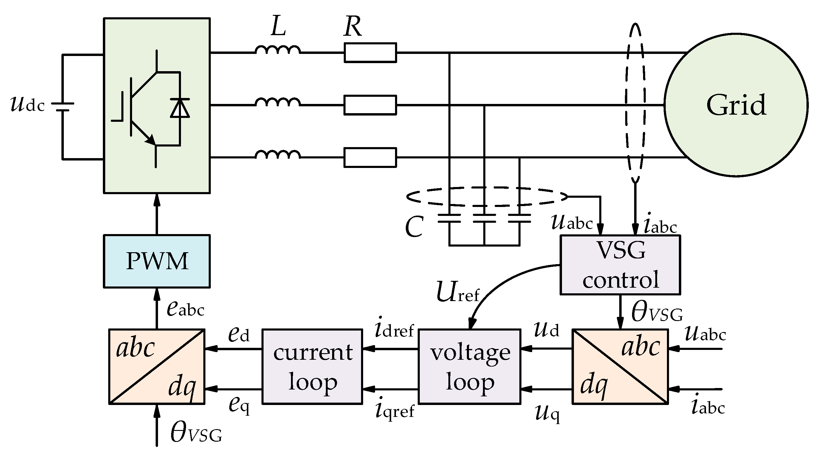
2. VSG Control Based on GFM Converter

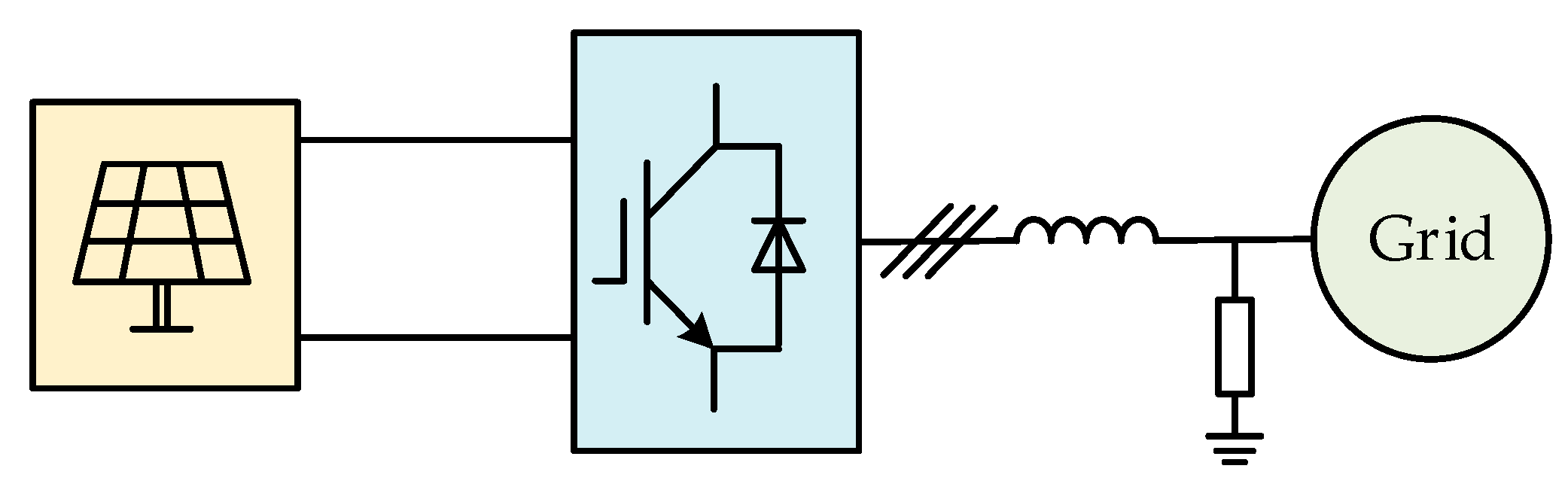
2.1. Control Principle of VSG Based on GFM System

Grid-forming converters do not require phase-locked loops. They can achieve active frequency and voltage regulation by emulating the synchronous control of synchronous generators, allowing them to theoretically operate in a grid composed entirely of power electronics. Currently, four main types of VSG control are used: droop control, virtual synchronous generator, matched control/inertial synchronous control, and virtual oscillator control. The schematic of the grid system using VSG control is illustrated in Figure 1 [10,11,12].

In VSG control using a grid-forming converter, directly synthesizing the generated voltage and phase angle as reference signals for the PWM link can lead to overcurrent issues and potential damage to switching devices during large perturbations, such as system faults, due to the absence of current limitation. Consequently, to address this issue, researchers have incorporated a dual inner-loop control of voltage and current into the virtual synchronous generator [13] to implement current limiting.

The grid-forming converter with VSG control exhibits voltage source characteristics. The detected filter capacitance voltage and inductor current are first transformed from abc to dq coordinates. These transformed signals are then fed into the outer VSG loop via the power calculation link and into the inner voltage and current loop. The inner loop generates the dq component of the converter’s reference voltage, which is subsequently transformed back into the three-phase reference voltage, e_abc, by the dq/abc transformation and used to generate a PWM signal.

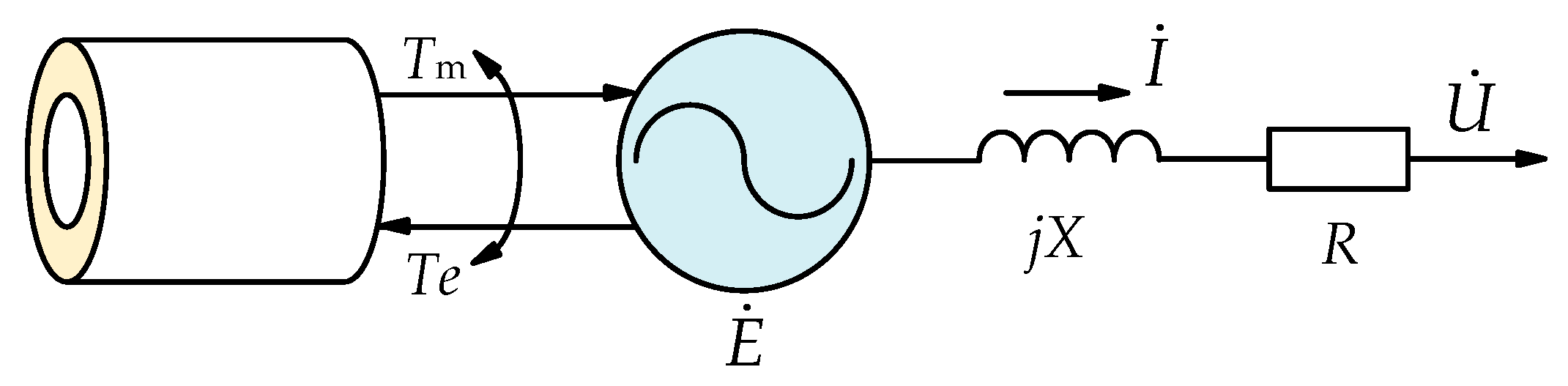
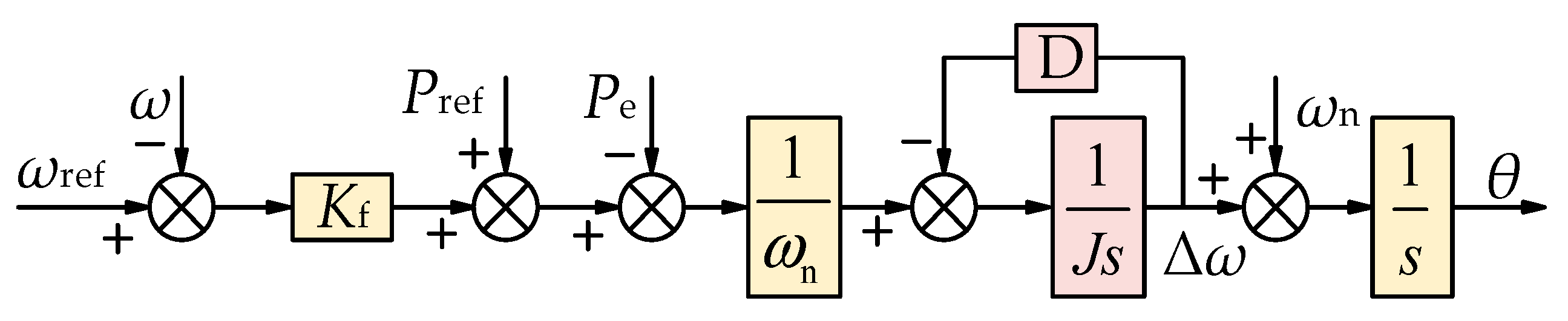
2.2. Principle and Characterization of VSG Control

Generally, the mathematical models of synchronous generators vary in complexity depending on the specific practical problem. This paper focuses on capturing only the basic response characteristics of synchronous generators, thus employing a simpler second-order electromechanical transient model. The simplified circuit diagram is illustrated in Figure 2.

T_m and T_e represent the mechanical and electromagnetic torques of the synchronous generator, respectively; E denotes the potential of the synchronous generator; and jX and R are its equivalent impedance components. This paper focuses on the hidden pole synchronous generator, and its stator voltage equation is as follows:

$$\left\{\begin{array}{l}{u}_{\mathrm{d}}=E_{\mathrm{d}}-L_{\mathrm{s}}{\displaystyle \frac{d{i}_{\mathrm{d}}}{dt}}+\omega L_{\mathrm{s}}{i}_{\mathrm{q}}-R_{\mathrm{s}}{i}_{\mathrm{d}}\\ u_{\mathrm{q}}=E_{\mathrm{q}}-L_{\mathrm{s}}{\displaystyle \frac{d{i}_{\mathrm{q}}}{dt}}+\omega L_{\mathrm{s}}{i}_{\mathrm{d}}-R_{\mathrm{s}}{i}_{\mathrm{q}}\end{array}\right.$$

(1)

where ω is the rotor angular velocity; u_d, u_q, i_d, and i_q are the voltage and current on the stator dq-axis, respectively; E_d, E_q are the components of the virtual potential on the dq-axis, respectively; and L_s and R_s are the stator inductance and resistance, respectively. The equation of motion of the synchronous generator rotor is

$$\left\{\begin{array}{l}J{\displaystyle \frac{d\omega }{dt}}=T_{\mathrm{m}}-T_{\mathrm{e}}-D\left(\omega -{\omega }_{\mathrm{N}}\right)\\ {\displaystyle \frac{d\theta }{dt}}=\omega \end{array}\right.$$

(2)

where T_m and T_e represent the mechanical torque and electromagnetic torque, respectively; ω and ω_n are the rotor angular velocity and rated angular velocity, respectively; θ is the virtual potential phase angle; J is the rotational inertia of the rotor; and D is the damping coefficient.

The VSG control circuit consists of several key components: a voltage–current acquisition module, a power calculation module, an active frequency controller, a reactive-voltage controller, a current reference generation module, a current-loop control module, and a PWM modulation module.

In the design of a VSG power–frequency controller, active frequency droop control is often used to emulate the governor function of a synchronous generator. This is represented by the following mathematical expression:

$$P_{\mathrm{n}}-P=k_{\mathrm{f}}\left(f-f_{\mathrm{n}}\right)$$

(3)

where k_f is the droop control factor. According to the principle of the VSG governor, calculate the difference between the current angular velocity of VSG and the rated angular velocity, multiply the difference with the droop coefficient, and finally add the result with the reference value of the active power to obtain the output mechanical power of VSG as follows:

$$P_{\mathrm{m}}-P_{\mathrm{ref}}=K_{\mathrm{f}}\left({\omega }_{\mathrm{ref}}-\omega \right)$$

(4)

where P_m is the VSG mechanical power; P_ref is the active power reference value; ω_ref and ω are the VSG rated angular velocity and actual angular velocity; and K_f is the active droop control factor.

The VSG power–frequency controller is formed by integrating the VSG governor with the rotor mechanical equation controller, as illustrated in Figure 3. The introduction of droop control, along with rotor virtual damping and virtual inertia, imparts the characteristics of primary frequency control found in synchronous machines. Additionally, the incorporation of inertia and damping enhances the system’s resistance to sudden frequency changes and severe power fluctuations, thereby improving overall system stability.

The voltage controller exhibits a similar relationship between reactive power and voltage as the power–frequency controller. However, since this paper primarily addresses the frequency control strategy, the voltage controller will not be discussed further.

3. Principle of LADRC for VSG Control Based on GFM Converter

3.1. Active Disturbance Rejection Control

Active disturbance rejection control (ADRC), proposed by Prof. Han Jingqing, is a control algorithm that does not rely on the object model. To address the challenges of ADRC parameter tuning, Prof. Gao Zhiqiang introduced linear auto-disturbance rejection control (LADRC). LADRC relates ADRC parameters to the frequencies of the controller and observer, thereby transforming parameter tuning into a bandwidth adjustment issue. LADRC comprises three components: the linear extended state observer (LESO), a proportional–derivative (PD) controller, and perturbation compensation [14,15,16]. Its schematic diagram is presented in Figure 4.

In the grid-forming system, the absence of a phase-locked loop eliminates the need to account for its dynamic effects. To stabilize the system frequency, a second-order linear self-immunity power–frequency controller is introduced. This controller ensures that the system frequency remains stable:

$$\ddot{y}=f\left(\dot{y},y,\omega \right)+b_{0}u=-a_1\dot{y}-a_{2}y+\omega \pm \left(b-b_0\right)u$$

(5)

where u is the system input; y is the output; ω is the perturbation; f is the total perturbation; a₁ and a₂ are the system parameters; and b is the controller gain. a₁, a₂ and b are unknown and b₀ ≈ b. Let x₁ = y and x₂ = $\dot{y}$. Its equation of state can be written as follows:

$$\left\{\begin{array}{l}{\dot{x}}_1=\dot{y}=x_2\\ {\dot{x}}_2=\dot{y}=x_3+b_{0}u\\ {\dot{x}}_3=\dot{f}\left(\dot{y},y,\omega \right)\end{array}\right.$$

(6)

where x₁, x₂, and x₃ are state variables, and x₃ is the dilated state. A linear expanded state observer (LESO) is built for the above equation as follows:

$$\left\{\begin{array}{l}{\dot{z}}_1=z_2+{\beta }_1\left(y-z_1\right)\\ {\dot{z}}_2=z_3+{\beta }_2\left(y-z_1\right)+b_{0}u\\ {\dot{z}}_3={\beta }_3\left(y-z_1\right)\end{array}\right.$$

(7)

where z₁, z₂, and z₃ are the observations of x₁, x₂, and x₃, respectively, and β₁, β₂, and β₃ are the observer gains. The LESO allows for the real-time tracking of the variables in the above equations: z₁ → y, z₂ → $\dot{y}$, and z₃ → f (y, $\dot{y}$, ω). Take:

$$u={\displaystyle \frac{-z_3+u_0}{b_0}}$$

(8)

According to the literature [17], the characteristic equation of LESO can be finally derived as follows:

$$\lambda \left(s\right)=s^3+{\beta }_1{s}^2+{\beta }_{2}s+{\beta }_3$$

(9)

Choosing the ideal characteristic equation λ (s) = (s + ω_o)³, we have

$${\beta }_1=3{\omega }_0,{\beta }_2=3{\omega }_0^2,{\beta }_3={\omega }_0^3$$

(10)

The resulting simplified structure of the LADRC is shown in Figure 5.

The problem of configuring the LADRC parameters reduces to the problem of selecting the observer bandwidth, ω_o, and the controller bandwidth, ω_c.

Focusing on the effect of the noise δ₀ of the observation quantity, y, and the perturbation, δ_c, at the input of the control quantity, u, on the LESO, the transfer function of the observation noise δ₀ is as follows:

$${\displaystyle \frac{z_1}{{\delta }_0}}={\displaystyle \frac{3{\omega }_0{s}^2+3{\omega }_0^{2}s+{\omega }_0^3}{{\left(s+{\omega }_0\right)}^3}}$$

(11)

As can be seen from Figure 6, with the increase in ω₀, the response speed of the system is accelerated, but at the same time, the high-frequency band gain increases, and the noise amplification becomes more obvious.

Similarly, the transfer function of the perturbation, δ_c, at the input can be obtained as follows:

$${\displaystyle \frac{z_1}{{\delta }_c}}={\displaystyle \frac{b_{0}s}{{\left(s+{\omega }_0\right)}^3}}$$

(12)

Taking b₀ = 10, the frequency domain characteristics are obtained as shown in Figure 7.

According to the frequency domain characteristics of observation noise, increasing the observer bandwidth, ω₀, reduces the phase lag of the tracked signal while having minimal impact on the gain in the high-frequency band.

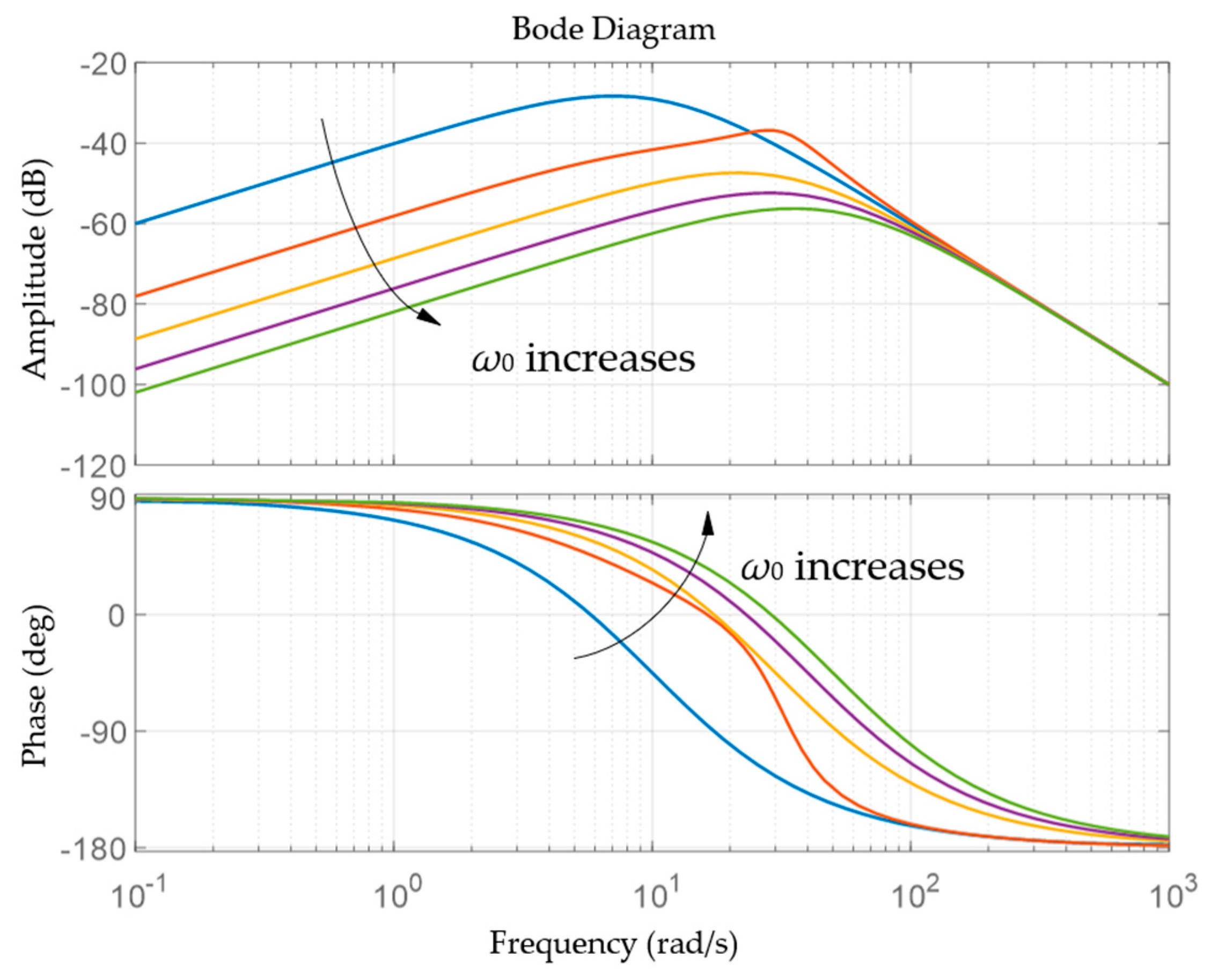
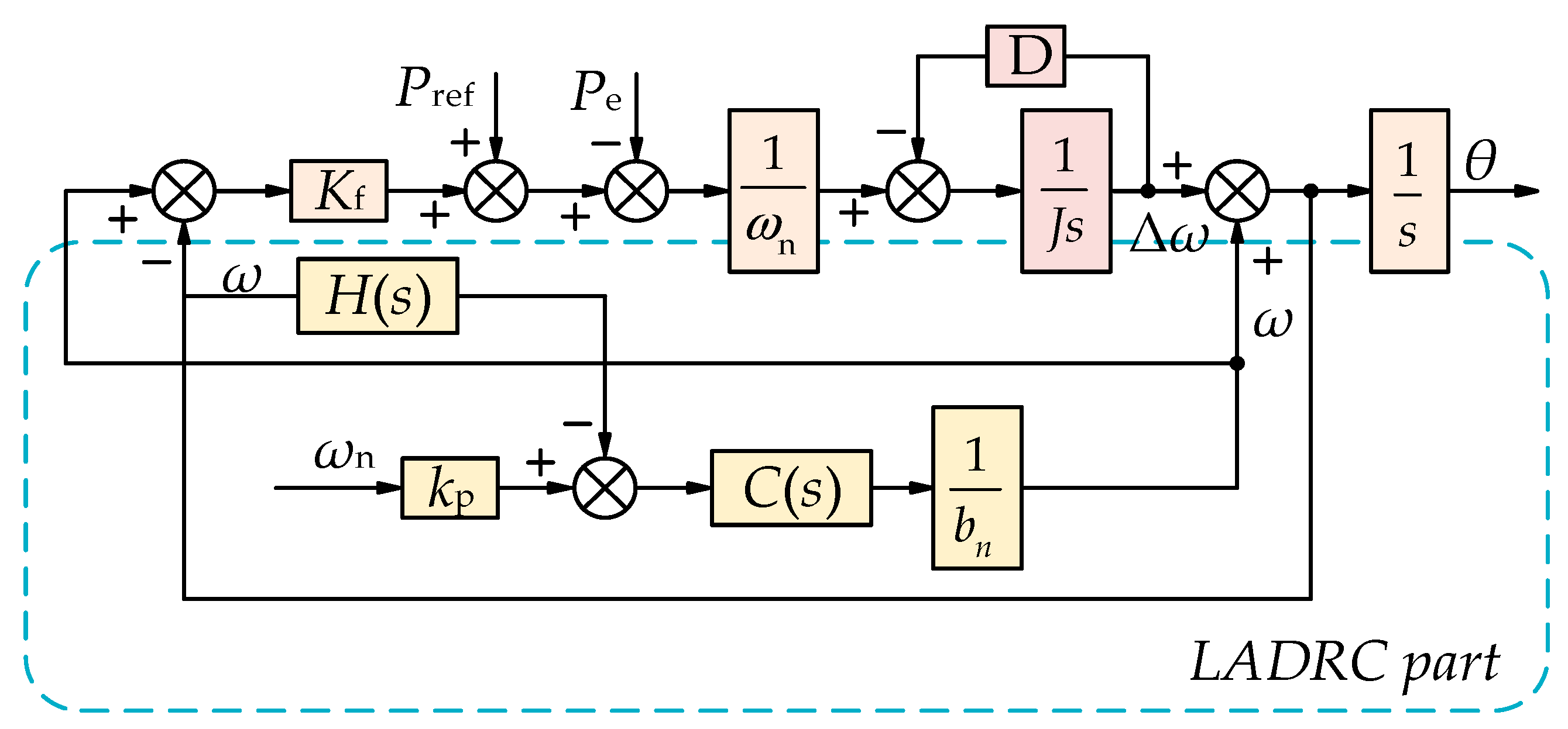
3.2. LADRC Power–Frequency Controller for VSG

The closed-loop transfer function expression for the output frequency of the conventional VSG with respect to the active power command value and the system frequency deviation value is as follows:

$$\left\{\begin{array}{l}\omega =G_{\omega \_P_{\mathrm{set}}}{P}_{\mathrm{set}}+G_{\omega \_P_{\mathrm{set}}}{P}_{\mathrm{out}}+{\omega }_{\mathrm{n}}\\ G_{\omega \_P_{\mathrm{set}}}={\displaystyle \frac{1}{J{\omega }_{\mathrm{n}}s+\left(D+k_{\mathrm{f}}\right){\omega }_{\mathrm{n}}}}\\ G_{\omega \_P_{\mathrm{set}}}={\displaystyle \frac{1}{\left[J{\omega }_{\mathrm{n}}s+\left(D+k_{\mathrm{f}}\right){\omega }_{\mathrm{n}}\right]\left(\tau s+1\right)}}\end{array}\right.$$

(13)

A Laplace inverse transform of the above equation yields the following:

$${\displaystyle \frac{d^2\omega }{d{t}^2}}={\displaystyle \frac{\left(D+k_{\mathrm{f}}\right){\omega }_{\mathrm{n}}}{J\tau }}+{\displaystyle \frac{P_{\mathrm{set}}-P_{\mathrm{out}}}{J{\omega }_{\mathrm{n}}\tau }}-{\displaystyle \frac{\left(D+k_{\mathrm{f}}\right)\omega }{J\tau }}-{\displaystyle \frac{\left[J{\omega }_{\mathrm{n}}+\left(D+k_{\mathrm{f}}\right){\omega }_{\mathrm{n}}\tau \right]}{J{\omega }_{\mathrm{n}}\tau }}{\displaystyle \frac{d\omega }{dt}}$$

(14)

It can be written as follows:

$${\displaystyle \frac{d^2\omega }{d{t}^2}}=bu+f\left(y,\dot{y},\omega \right),u={\omega }_{\mathrm{n}}$$

(15)

Combined with the VSG power–frequency controller, the principle of LADRC power–frequency controller can be obtained, as shown in Figure 8:

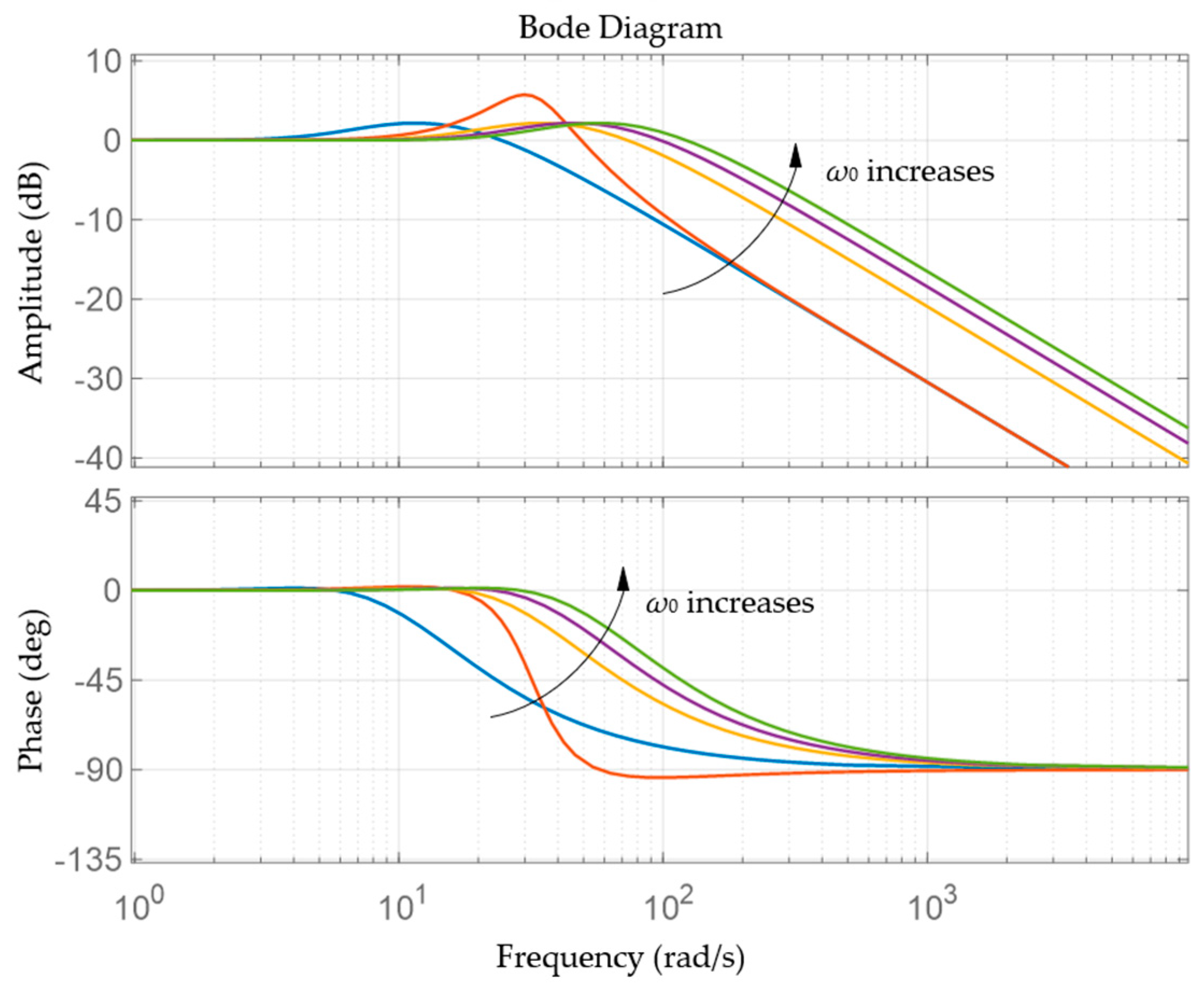
3.3. Parameter Calibration

The rectification method used in this paper mainly refers to the literature [18]. According to the analysis above, the parameters b, ω_o and ω_c need to be chosen for the rectification in order to make the LADRC algorithm give the best performance. It can be obtained from Equations (14) and (15).

This paper primarily adopts the rectification method described in the literature [18]. Based on the preceding analysis, the parameters b, ω_o and ω_c must be selected to optimize the performance of the LADRC algorithm. These parameters can be determined from Equations (14) and (15):

$$b={\displaystyle \frac{\left(D+k_{\mathrm{f}}\right)}{J\tau }}$$

(16)

The system’s stability is analyzed using the Lienard–Chipard stability criterion, which requires that the coefficients of the characteristic equation and the parity order of its determinant be positive. The closed-loop transfer function for the control system is derived from Figure 8 as follows:

$$\left\{\begin{array}{l}\omega ={\displaystyle \frac{M\left(s\right)}{Q\left(s\right)}}{P}_{\mathrm{out}}\left(s\right)+{\displaystyle \frac{N\left(s\right)}{Q\left(s\right)}}{P}_{\mathrm{ref}}\left(s\right)+{\displaystyle \frac{P\left(s\right)}{Q\left(s\right)}}{\omega }_{\mathrm{n}}\left(s\right)\\ M\left(s\right)=-b{s}^3-b\left({\beta }_1+k_{\mathrm{d}}\right)s^2-b\left({\beta }_1{k}_{\mathrm{d}}+{\beta }_2+k_{\mathrm{p}}\right)s\\ N\left(s\right)=b\left(\tau s+1\right)\\ P\left(s\right)=k_{\mathrm{p}}C\left(s\right)\left(\tau s+1\right)\left[J{\omega }_{\mathrm{n}}s+\left(D+k_{\mathrm{f}}{\omega }_{\mathrm{n}}\right)\right]\\ Q\left(s\right)=q_1{s}^5+q_2{s}^4+q_3{s}^3+q_4{s}^2+q_{5}s+q_6\end{array}\right.$$

(17)

where ω(s), P_out(s), P_ref(s) and ω_n(s) are their forms in the complex frequency domain, respectively. The characteristic equations are derived as follows:

$$\left\{\begin{array}{l}{q}_1{s}^5+q_2{s}^4+q_3{s}^3+q_4{s}^2+q_{5}s+q_6=0\\ q_1=J{\omega }_{\mathrm{n}}b\tau \\ q_2=b\left(J{\omega }_{\mathrm{n}}+D{\omega }_{\mathrm{n}}\tau \right)+J{\omega }_{\mathrm{n}}\tau \left({\beta }_3+\right.b{k}_{\mathrm{d}}+b{\beta }_1+k_{\mathrm{d}}{\beta }_2+k_{\mathrm{p}}{\beta }_1)\\ q_3=\left(J{\omega }_{\mathrm{n}}+D{\omega }_{\mathrm{n}}\tau \right)\left({\beta }_3+b{k}_{\mathrm{d}}+b{\beta }_1+k_{\mathrm{d}}{\beta }_2+k_{\mathrm{p}}{\beta }_1\right)+D{\omega }_{\mathrm{n}}b+J{\omega }_{\mathrm{n}}\tau \left(k_{\mathrm{d}}{\beta }_3+b{k}_{\mathrm{p}}+b{k}_{\mathrm{d}}{\beta }_1+b{\beta }_2+k_{\mathrm{d}}{\beta }_2\right)\\ q_4=\left(J{\omega }_{\mathrm{n}}+D{\omega }_{\mathrm{n}}\tau \right)\left(k_{\mathrm{d}}{\beta }_3+b{k}_{\mathrm{p}}+b{k}_{\mathrm{d}}{\beta }_1+b{\beta }_2+k_{\mathrm{p}}{\beta }_2\right)+D{\omega }_{\mathrm{n}}\left({\beta }_3+b{k}_{\mathrm{d}}+b{\beta }_1+k_{\mathrm{d}}{\beta }_2+k_{\mathrm{p}}{\beta }_1\right)+J{\omega }_{\mathrm{n}}\tau k_{\mathrm{p}}{\beta }_3\\ q_5=k_{\mathrm{p}}{\beta }_3\left(J{\omega }_{\mathrm{n}}+D{\omega }_{\mathrm{n}}\tau \right)+D{\omega }_{\mathrm{n}}\left(k_{\mathrm{d}}{\beta }_3+b{k}_{\mathrm{p}}\right.+b{k}_{\mathrm{d}}{\beta }_1+b{\beta }_2+k_{\mathrm{p}}{\beta }_2)\\ q_6=D{\omega }_{\mathrm{n}}{k}_{\mathrm{p}}{\beta }_3\end{array}\right.$$

(18)

From the above equation, it can be obtained that q₁~q₆ are all greater than zero, so the condition of system stability can be simplified as follows:

$$\left(q_2{q}_3-q_1{q}_4\right)\left(q_4{q}_5-q_3{q}_6\right)-{\left(q_2{q}_5-q_1{q}_6\right)}^2>0$$

(19)

Therefore, the relationship between ω_c and ω₀ can be initially established based on the stabilization constraints from the previous equations. However, the Lienard–Chipard stability criterion alone does not indicate the degree of stability. To obtain more reliable parameters, it is necessary to evaluate how different parameters affect controller performance. This analysis integrates the effects of varying ω_c and ω₀ on the controller’s performance.

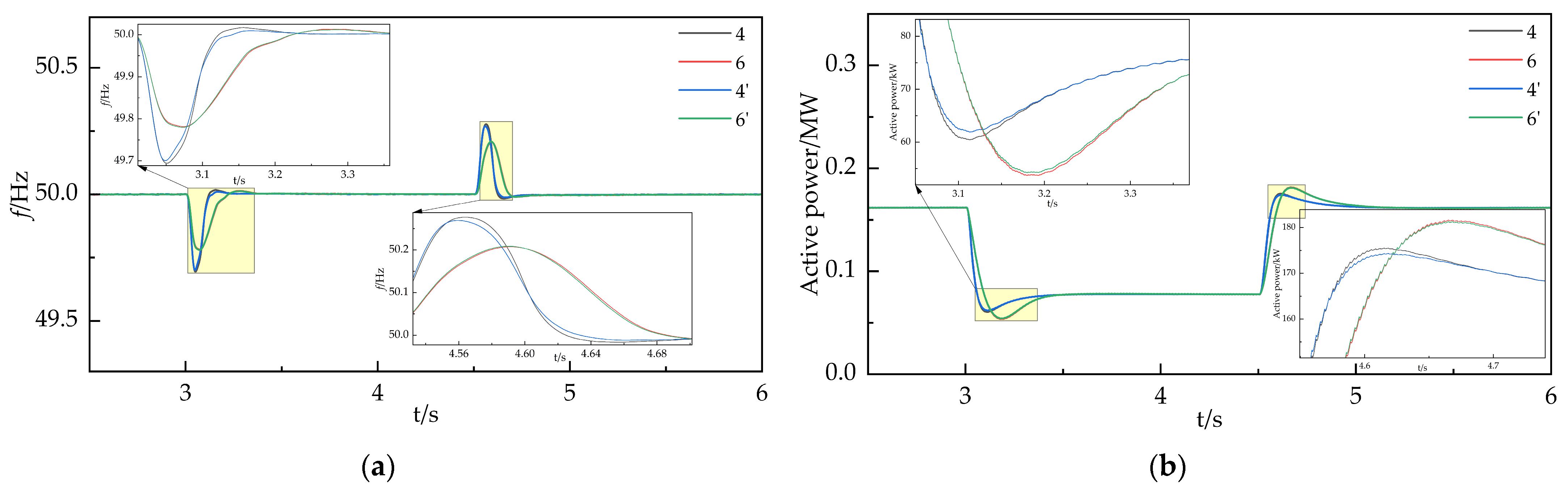
3.4. Simulation Result and Analysis

The MATLAB/Simulink simulation platform is utilized to construct a grid-forming standalone infinity PV grid-connected system, as illustrated in Figure 9. In this system, the maximum power point tracking (MPPT) of the PV system employs the perturbation observation method, while the inverter control implements both traditional VSG control and LADRC-optimized VSG control.

Table 2. System parameters.

ESO Parameters	k1	k2	k3
value	300	30,000	1,000,000
ESO Parameters	ω0	ωc	b
value	100	800	500
Conditions	LADRC	J	D
1	No	0.2	30
2		0.2	50
3		1	50
4	Yes	0.2	30
5		0.2	50
6		1	50

shows the parameters of the single-machine infinity generation system.

Scenario 1:

The temperature of the photovoltaic panel is set to 25 °C. The light intensity is programmed to decrease from 1600 W/m² to 800 W/m² at 3 s, then increase back to 1600 W/m² at 4.5 s. The total simulation duration is 6 s. The simulation results for system frequency and active power are shown in Figure 10.

From Figure 10a, comparing simulation condition 1 with 4, 2 with 5, and 3 with 6, it is evident that the LADRC-optimized VSG control performs better in managing frequency fluctuations compared to traditional VSG control during system perturbations. Additionally, comparisons between conditions 2 and 3, as well as 5 and 6, reveal that appropriately increasing rotational inertia enhances the system’s frequency robustness and reduces overshoot. Furthermore, comparing conditions 1 with 2 and 4 with 5 shows that increasing the damping coefficient also improves the robustness of the system’s frequency.

Figure 10b presents the simulation results for system active power. The figure demonstrates that LADRC-optimized VSG control effectively enhances the output active power curve and improves the system’s robustness.

Scenario 2:

The PV panel temperature is set to 25 °C with a constant light intensity of 1200 W/m². A three-phase ground short-circuit fault is introduced in the grid-connected main line at 0.1 s and removed at 0.2 s. The frequency and active power simulation results after 0.2 s, comparing simulation conditions 2, 3, 5, and 6, are shown in Figure 11.

The curves in Scenario 2 illustrate the system’s recovery to a steady state following a three-phase short-circuit fault. Figure 11 confirms that LADRC-optimized VSG control enhances system stability.

4. Study of PSO-LADRC Strategy

4.1. Fundamentals of PSO-LADRC Strategy

To further enhance the control strategy for the combination of LADRC and VSG in the GFM system, the particle swarm optimization (PSO) algorithm is introduced to determine the optimal values for the relevant control parameters.

The particle swarm optimization (PSO) algorithm is a global optimization technique inspired by the foraging behavior of bird flocks. It adjusts two attributes of particles: position and speed, and finally converges them to the optimal solution through the movement of multiple particles in parameter space and the exchange of information.

From the analysis, it is evident that ω_o, ω_c, and b are key parameters influencing the performance of the LADRC algorithm. The particle swarm optimization (PSO) algorithm can be employed to determine the optimal values for these parameters. Therefore, this paper explores a parameter space of 3. The basic principles of the PSO algorithm are as follows:

1.

Particle Position Representation Parameter: In the PSO algorithm, each particle’s state is represented by a d-dimensional vector, which indicates the particle’s current position. The position vector of a particle is defined as

$$x_{\mathrm{i}}=\left(x_{\mathrm{i}1},x_{\mathrm{i}2},\cdots ,x_{\mathrm{id}}\right)$$

(20)

where x_i denotes the position of the i-th particle in d-dimensional space.

2.

Particle Velocity Indicates Search Direction: The velocity of a particle represents the direction in which the particle searches within the d-dimensional space. The velocity vector of a particle is defined as

$$v_{\mathrm{i}}=\left(v_{\mathrm{i}1},v_{\mathrm{i}2},\cdots ,v_{\mathrm{id}}\right)$$

(21)

where v_i denotes the velocity of the i-th particle.

3.

Each Particle Records its Own Best Position and Fitness: Each particle tracks its best found position and the corresponding fitness value. This allows each particle to retain good local solutions. The optimal position vector is denoted as

$$p_{\mathrm{i}}=\left(p_{\mathrm{i}1},p_{\mathrm{i}2},\cdots ,p_{\mathrm{id}}\right)$$

(22)

where p_i denotes the optimal position found by the i-th particle.

4.

Global Optimal Position for the Entire Population: The global optimal position is recorded across all particles in the population. The global optimal position vector is denoted as

$$g_{\mathrm{i}}=\left(g_{\mathrm{i}1},g_{\mathrm{i}2},\cdots ,g_{\mathrm{id}}\right)$$

(23)

5.

Updates Speed and Position Using Current Speed and Historical Information: The speed and position are updated based on the current speed and historical data. The speed update formula is given by

$$v_{\mathrm{i}}\left(t+1\right)=w{v}_{\mathrm{i}}\left(t\right)+c_1{r}_1\left(p_{\mathrm{i}}\left(t\right)-x_{\mathrm{i}}\left(t\right)\right)+c_2{r}_2\left(g\left(t\right)-x_{\mathrm{i}}\left(t\right)\right)$$

(24)

where w is the inertia weight, balancing the global search and local convergence abilities of the particle swarm; c₁ and c₂ are the learning factors for individual and collective experiences, respectively; and r₁ and r₂ are random numbers between 0 and 1.

The position update formula is given by

$$x_{\mathrm{i}}\left(t+1\right)=x_{\mathrm{i}}\left(t\right)+v_{\mathrm{i}}\left(t+1\right)$$

(25)

As discussed, the particle swarm optimization (PSO) algorithm iteratively updates and refines the objective function, progressively converging to the global optimal solution.

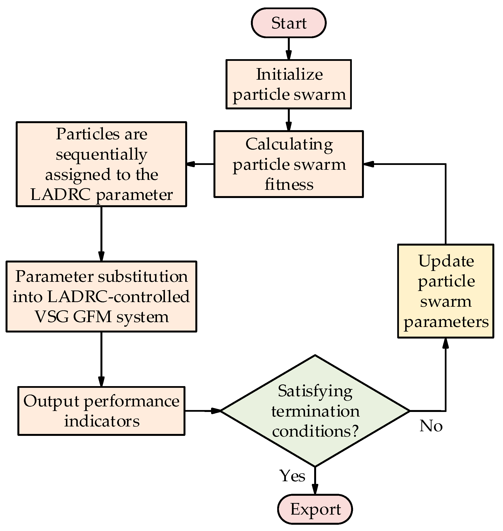
4.2. PSO-LADRC Parameter Calibration

The flowchart of the PSO-LADRC algorithm is illustrated in Figure 12.

To achieve optimal dynamic control performance, the objective function for parameter adjustment is set as half of the squared output error of the position loop. Additionally, to prevent excessive control volume, the squared input of the control volume is included, resulting in the final fitness function given by

$$F={\displaystyle \frac{1}{2}}{\omega }^2+{\displaystyle \frac{1}{2}}{u}^2$$

(26)

where ω represents the final output error of the system frequency, and u denotes the control input. After each iteration, the minimum value of the fitness function is determined by adjusting the controller parameters, which is then considered the best fitness value.

The parameterization procedure is as follows:

• Initialize Relevant Parameters: Set the particle swarm’s size, iteration number, and spatial dimensions. Randomly initialize parameters such as the position and velocity vectors of the particles, and also initialize the parameters of the LADRC.
• Calculate the Fitness Function Value: assign the particle swarm’s position vectors to the LADRC and compute the fitness function value for each particle based on its current position vector.
• Update Self and Global Best Positions: For each particle, if the current fitness function value is better than its personal best, update the particle’s personal best position. Additionally, if the current fitness function value is better than the global best, update the global best position.
• Updates to the particle velocity: If v_id (t + 1) ≤ v_min, then set v_id (t + 1) = v_min. If v_id (t + 1) ≥ v_max, then set v_id (t + 1) = v_max.
• Update the particle position: If x_id (t + 1) ≤ x_min, then set x_id (t + 1) = x_min. If x_id (t + 1) ≥ x_max, then set x_id (t + 1) = x_max.
• Check Termination Condition: If the preset number of iterations is reached, terminate the algorithm and output the controller parameters. Otherwise, return to step 2.

4.3. Simulation Result and Analysis

The simulation study is conducted using the GFM stand-alone infinity PV grid-connected system described in Section 3.4. Inverter control is tested with both LADRC-optimized-VSG control and PSO-LADRC-optimized VSG control.

The simulation study utilizes the GFM stand-alone infinity PV grid-connected system described in Section 3.4. Inverter control is evaluated using both LADRC-optimized VSG control and PSO-LADRC-optimized VSG control.

Scenario 1:

Simulation conditions 4 and 6 correspond to the curves obtained with LADRC-optimized VSG control, using parameters J = 0.2, D = 30 and J = 1, D = 50, as described in Section 3.4. Simulation conditions 4′ and 6′ represent the curves with PSO-LADRC-optimized VSG control under the same parameters as conditions 4 and 6. The simulation results for system frequency and active power are shown in Figure 13.

Since the particle swarm algorithm has some randomness, the values from of each iteration are different. The iterated values ω₀ = 146.5, ω_c = 85.1, and b = 55,903.3 were used for the simulation of PSO-LADRC-optimized VSG control. The LADRC-optimized VSG control remains in the same conditions as in Section 3.4. According to the literature [18], the system is in a steady state.

Due to the inherent randomness of the particle swarm algorithm, the values from each iteration can vary. For this simulation, the iterated parameters are ω₀ = 146.5, ω_c = 85.1, and b = 55,903.3 for the PSO-LADRC-optimized VSG control. The LADRC-optimized VSG control conditions remain as described in Section 3.4. According to the literature [18], the system reaches a steady state.

Figure 13a shows that PSO-LADRC-optimized VSG control enhances the system’s frequency regulation capability more effectively than using LADRC-optimized VSG control alone, resulting in greater system robustness. Additionally, the values of J and D impact the optimization effectiveness of system robustness, as detailed in

Table 3. ΔFN values for different values of J and D.

Parameters	J	D	ΔFN
1	0.2	30	0.009053195
2	0.5	30	0.013404251
3	1	30	0.014185879
4	0.2	40	0.008924131
5	0.2	50	0.008364361

after several simulations. The difference in frequency nadir (FN) values after 3 s, calculated for different J and D values using LADRC and PSO-LADRC strategies, is used to obtain ΔFN values. This is used to verify the effect of J and D values on the system.

Table 3 shows that ΔFN increases as J increases and D decreases. In other words, the optimization effect of the PSO-LADRC strategy on LADRC becomes more pronounced with higher J values and lower D values.

Figure 13b presents the simulation results for system active power. Compared to LADRC-optimized VSG control, PSO-LADRC-optimized VSG control further optimizes the system’s output active power curve, thereby enhancing system robustness.

Scenario 2:

The PV panel temperature is set to 25 °C and the light intensity to 1200 W/m², both held constant. A three-phase ground short-circuit fault is applied to the grid-connected main line at 0.1 s and cleared at 0.2 s. The simulation results for conditions 5, 6, 5′, and 6′ are compared, with frequency and active power shown after 0.2 s in Figure 14.

Figure 14 demonstrates that PSO-LADRC-optimized VSG control enhances system stability more effectively than LADRC-optimized VSG control.

However, the PSO algorithm has limitations, including a tendency to get stuck in local optima and its slower convergence speed. To address these issues, the particle swarm algorithm is run for multiple iterations and analyzed through simulations. The working condition 4′ described above is selected, and the frequency nadir values after 3 s are recorded.

Table 4. FN values after multiple iterations.

Number of Iterations	ωo	ωc	b	FN
1	146.5	85.1	55,903.3	49.70028
2	276.0	81.5	16,218.3	49.70102
3	301.5	5.9	42,288.6	49.70069
4	163.5	98.8	63,118.9	49.69931
5	285.9	50.4	40,672.8	49.70171
6	318.0	14.0	67,227.1	49.69891

presents the FN values obtained from these iterations.

Table 4 shows that the variation in FN across multiple iterations is less than 0.1%, which is negligible. Thus, the limitations of the particle swarm algorithm do not significantly impact the optimization of system robustness.

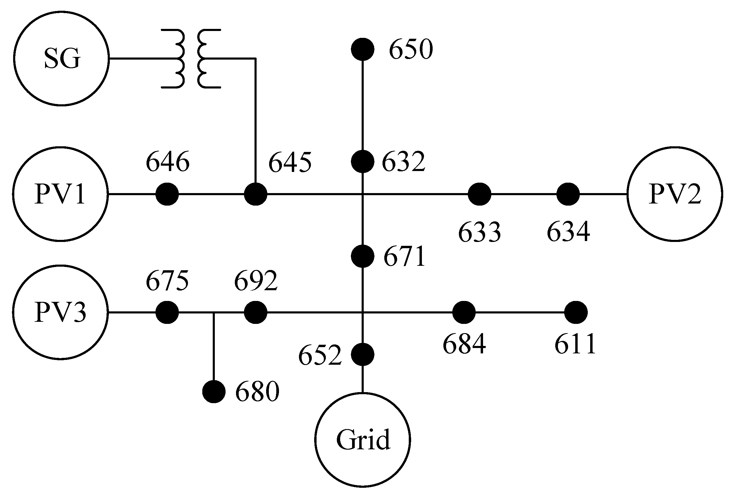
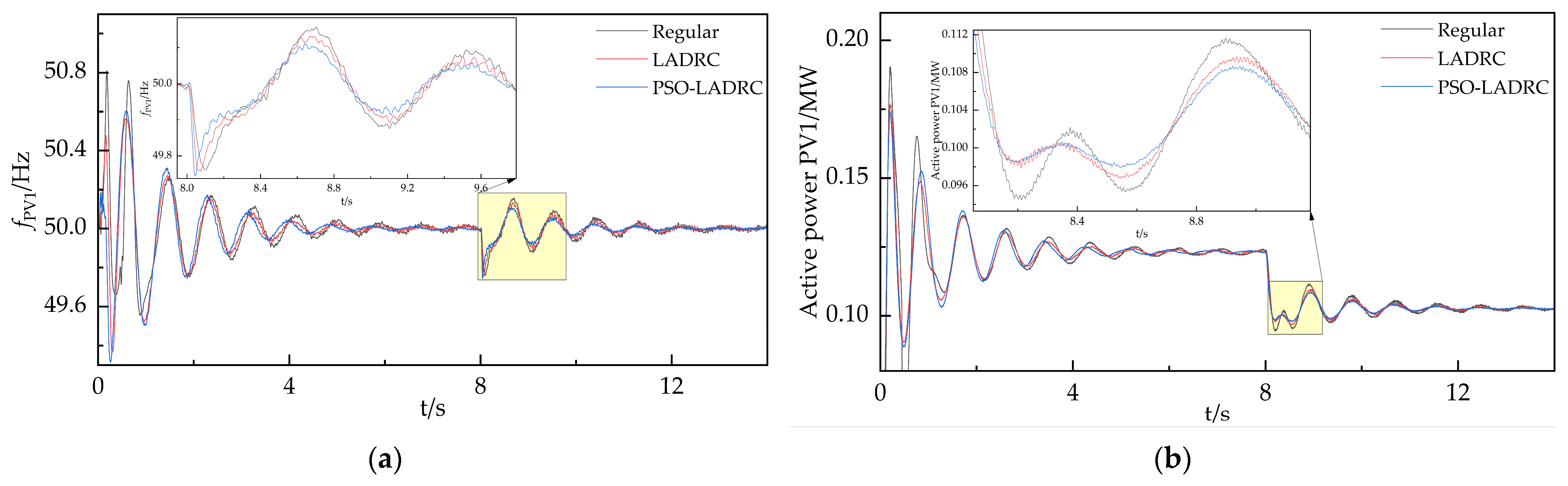
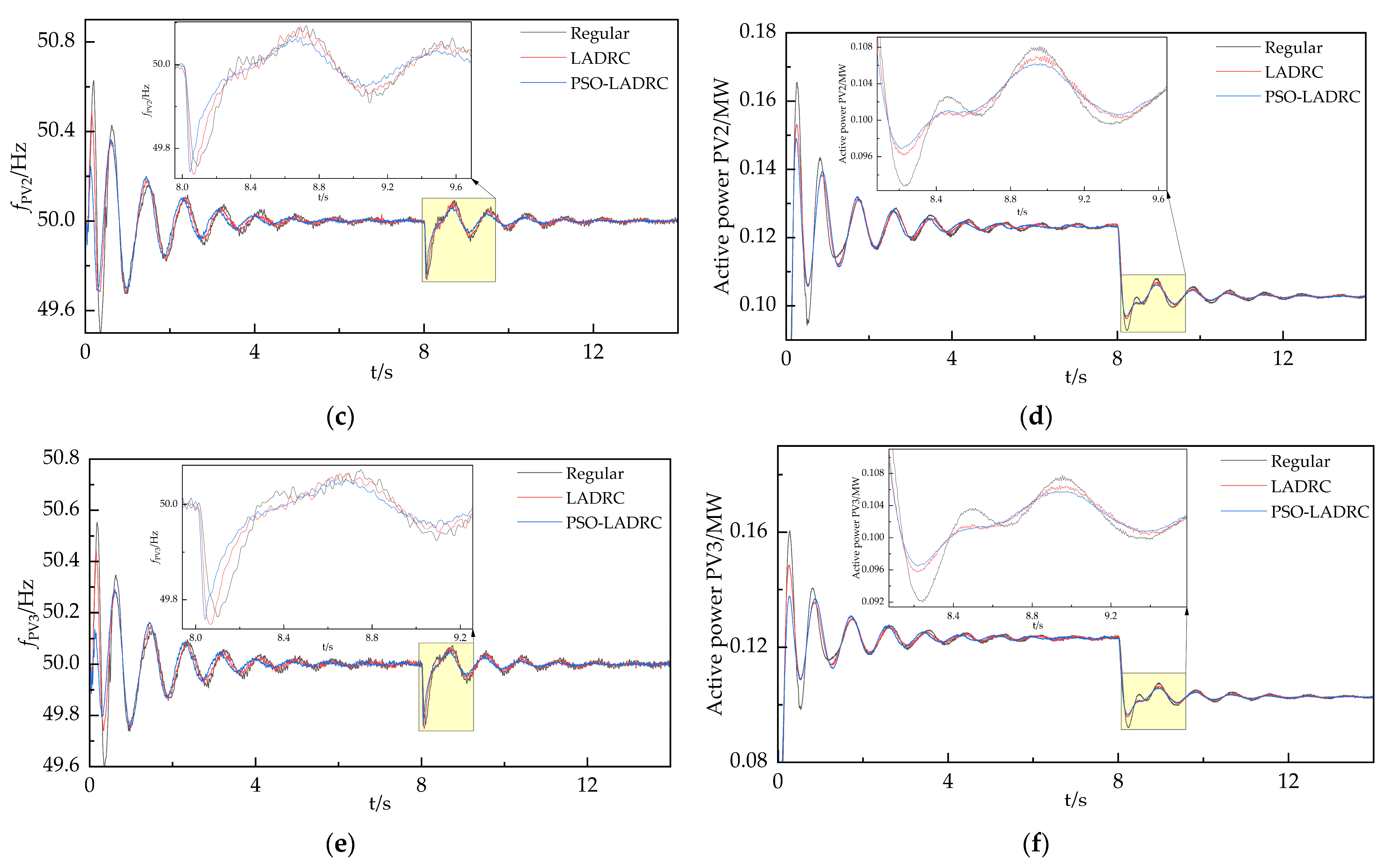
5. Simulation Results and Analysis of Large Power System

To verify the general applicability of the proposed control strategy, it is implemented in a large power system with multiple VSG units. Figure 15 illustrates the structural topology of multiple grid-forming distributed PVs integrated into the IEEE 13-bus system. The three identical PV units are simulated and analyzed under three different control methods: regular control, LADRC, and PSO-LADRC.

The PV penetration rate indicates the proportion of photovoltaic (PV) capacity connected to the system. The photovoltaic capacity penetration (CP) is calculated using the following formula:

$${\lambda }_{\mathrm{CP}}={\displaystyle \frac{P_{\mathrm{PV}\max }}{P_{\mathrm{load}\max }}}\times 100\%$$

(27)

where P_{PV max} represents the maximum annual generation power of the distributed PV system, and P_{load max} denotes the maximum annual load in the region.

Scenario 1:

The settings for PV1, PV2, and PV3 are identical: J = 0.2, D = 30, and parameters ω₀, ω_c and b are specified in Section 3.4. The temperature is maintained at a constant 25 °C. The light intensity is initially set to 1200 W/m², then reduced to 1000 W/m² after 8 s, and held at this level for the remainder of the simulation. P_{load max} is 1.045 MW. At 1200 W/m², P_{load max} is 0.36 MW with λ_CP of 34.4%. At 1000 W/m², P_{load max} is 0.3 MW and λ_CP is 28.7%. The frequency and active power curves for PV1, PV2, and PV3 are illustrated in Figure 16.

Figure 16a,c,e shows that the LADRC and PSO-LADRC strategies are well suited for large power systems with multiple VSG units and high PV penetration. When PV unit output decreases, both LADRC and PSO-LADRC strategies reduce system fluctuation amplitude and stabilize the system frequency more effectively compared to conventional control strategies, thus improving system robustness. Figure 16b,d,f further illustrate that PSO-LADRC stabilizes the active power of PV output more rapidly than LADRC, significantly enhancing system robustness.

Scenario 2:

This simulation investigates high power load shedding in a large power system with multiple VSG units and high PV penetration. The settings for PV1, PV2, and PV3 are identical: J = 0.2, D = 30, and parameters ω₀, ω_c and b are specified in Section 3.4. The temperature is maintained at a constant 25 °C, and the light intensity is kept constant at 1200 W/m². At 8 s, the system reduces the load by 0.145 MW, which remains constant for the rest of the simulation. When P_{load max} is 1.045 MW, λ_CP = 34.4%. When P_{load max} is reduced to 0.9 MW, λ_CP increases to 40%. The frequency and active power curves for PV1, PV2, and PV3 are illustrated in Figure 17.

Figure 17 shows that in a large power system with multiple VSG units and high PV penetration, LADRC and PSO-LADRC strategies stabilize the frequency and active power output of PV units more rapidly than conventional control strategies during high power load shedding. This improvement enhances the system’s resilience to disturbances.

6. Conclusions

This paper investigates the LADRC strategy applied to VSG GFM converters to address the issue of frequent frequency fluctuations in GFM grids. Additionally, a PSO-LADRC strategy is proposed, which incorporates the PSO algorithm to enhance system robustness. The effectiveness of these control strategies is validated through simulation analysis. The main conclusions are as follows:

• A VSG converter-based on GFM power grid is established and its structural principles are studied and analyzed.
• An LADRC for VSGs is proposed and implemented in a VSG converter for a GFM grid. This approach enhances system robustness during frequency fluctuations and improves stability following faults. The effectiveness of this controller is confirmed through simulation.
• The PSO-LADRC algorithm, which incorporates particle swarm optimization, is proposed and applied to the VSG converter in a GFM grid. This approach further enhances system robustness and stability. An analysis over several iterations confirms that the limitations of particle swarm optimization do not undermine the effectiveness of the control strategy.
• To evaluate the effectiveness of control strategies in large-scale power systems with multiple VSG units and high PV penetration, we developed simulation models. We verified the generalization of LADRC and PSO-LADRC strategies for system robustness optimization under various disturbances and PV penetration levels.

References

1. Zhang, X.; Ruan, X.; Zhong, Q. Improving the Stability of Cascaded DC/DC Converter Systems via Shaping the Input Impedance of the Load Converter with a Parallel or Series Virtual Impedance. IEEE Trans. Ind. Electron. 2015, 62, 7499–7512. [Google Scholar] [CrossRef]
2. Wang, K.; Qi, C.; Huang, X.; Li, G. Large disturbance stability evaluation of interconnected multi-inverter power grids with VSG model. J. Eng. 2017, 13, 2483–2488. [Google Scholar] [CrossRef]
3. Matevosyan, J.; Badrzadeh, B.; Prevost, T.; Quitmann, E.; Ramasubramanian, D.; Urdal, H.; Achilles, S.; MacDowell, J.; Huang, S.H.; Vital, V.; et al. Grid-Forming Inverters: Are They the Key for High Renewable Penetration. IEEE Power Energy Mag. 2019, 17, 89–98. [Google Scholar] [CrossRef]
4. Guo, L.; Xu, Z.; Jin, N.; Li, Y.; Wang, W. A weighted voltage model predictive control method for a virtual synchronous generator with enhanced parameter robustness. Prot. Control Mod. Power Syst. 2021, 6, 482–492. [Google Scholar] [CrossRef]
5. Wen, C.; Chen, D.; Hu, C.; Piao, Z.; Zhou, J. Self-adaptive Control of Rotational Inertia and Damping Coefficient of VSG for Converters in Microgrid. Autom. Electr. Power Syst. 2018, 42, 175–186. [Google Scholar]
6. Yu, Y.; Hu, X. Active Disturbance Rejection Control Strategy for Grid-Connected Photovoltaic Inverter Based on Virtual Synchronous Generator. IEEE Access 2019, 7, 17328–17336. [Google Scholar] [CrossRef]
7. Yu, J.; Sun, W.; Yu, J.; Wang, Y. Virtual synchronous generator control of a grid-connected inverter based on adaptive inertia. Power Syst. Prot. Control 2022, 50, 137–144. [Google Scholar]
8. Li, D.; Zhu, Q.; Lin, S.; Bian, X.Y. A self-adaptive inertia and damping combination control of VSG to support frequency stability. IEEE Trans. Energy Convers. 2016, 32, 397–398. [Google Scholar] [CrossRef]
9. Choopani, M.; Hosseinian, S.H.; Vahidi, B. New transient stability and LVRT improvement of multi-VSG grids using the frequency of the center of inertia. IEEE Trans. Power Syst. 2019, 35, 527–538. [Google Scholar] [CrossRef]
10. Zhang, Y.; Zhu, J.; Dong, X.; Zhao, P.; Ge, P.; Zhang, X. A control strategy for smooth power tracking of a grid-connected virtual synchronous generator based on linear active disturbance rejection control. Energies 2019, 14, 3024. [Google Scholar] [CrossRef]
11. Yang, Y.; Xu, J.; Li, C.; Zhang, W.; Wu, Q.; Wen, M.; Blaabjerg, F. A New Virtual Inductance Control Method for Frequency Stabilization of Grid-Forming Virtual Synchronous Generators. IEEE Trans. Ind. Electron. 2022, 70, 441–451. [Google Scholar] [CrossRef]
12. Li, M.; Wang, Y.; Xu, N.; Niu, R.; Lei, W. Virtual synchronous generator control strategy based on bandpass damping power feedback. Trans. China Electrotech. Soc. 2018, 33, 2176–2185. [Google Scholar]
13. D’Arco, S.; Suul, J.A. Virtual Synchronous Machines Classification of Implementations and Analysis of Equivalence to Droop Controllers for Microgrids. In Proceedings of the 2013 IEEE Grenoble Conference, Powertech, Grenoble, France, 16–20 June 2013; IEEE: Piscataway, NJ, USA, 2013. [Google Scholar]
14. Han, J.Q. From PID to active disturbance rejection control. IEEE Trans. Ind. Electron. 2009, 56, 900–906. [Google Scholar] [CrossRef]
15. Wu, D.; Chen, K. Frequency-domain analysis of nonlinear active disturbance rejection control via the describing function method. IEEE Trans. Ind. Electron. 2013, 60, 3906–3914. [Google Scholar] [CrossRef]
16. Guo, B.Z.; Jin, F.F. Sliding mode and active disturbance rejection control to stabilization of one-dimensional anti-stable wave equations subject to disturbance in boundary input. IEEE Trans. Autom. Control 2013, 58, 1269–1274. [Google Scholar] [CrossRef]
17. Yuan, D.; Ma, X.; Zeng, Q.; Qiu, X. Research on frequency-band characteristics and parameters configuration of linear active disturbance rejection control for second-order systems. Control Theory Technol. 2013, 30, 1630–1640. [Google Scholar]
18. Liang, Q.; Wang, C.; Pan, J.W.; Wei, Y.H.; Wang, Y. Parameter identification of b0 and parameter tuning law in linear active disturbance rejection control. Control Decis. 2015, 30, 1691–1695. [Google Scholar]
Figure 1. Schematic diagram of VSG-GFM system.
Electronics 13 03017 g001
Figure 2. Simplified circuit diagram of synchronous generator.
Electronics 13 03017 g002
Figure 3. Structure of VSG P-f controller.
Electronics 13 03017 g003
Figure 4. Schematic diagram of LADRC.
Electronics 13 03017 g004
Figure 5. Simplified structure of LADRC.
Electronics 13 03017 g005
Figure 6. Frequency domain characteristics of observation noise.
Electronics 13 03017 g006
Figure 7. Frequency domain characteristics of input channel disturbance.
Electronics 13 03017 g007
Figure 8. Active disturbance rejection control structure of VSG P-f controller.
Electronics 13 03017 g008
Figure 9. GFM single-unit infinity PV system.
Electronics 13 03017 g009
Figure 10. System simulation curve at 2.5–6 s for scenario 1: (a) frequency curve of the system; (b) active power curve of the system.
Electronics 13 03017 g010
Figure 11. System simulation curve at 0.2–1 s for scenario 1: (a) frequency curve of the system; (b) active power curve of the system.
Electronics 13 03017 g011
Figure 12. Flowchart of PSO-LADRC algorithm.
Electronics 13 03017 g012
Figure 13. System simulation curve at 2.5-6 s for scenario 2: (a) frequency curve of the system; (b) active power curve of the system.
Electronics 13 03017 g013
Figure 14. System simulation curve at 0.2-1 s for scenario 2: (a) frequency curve of the system; (b) active power curve of the system.
Electronics 13 03017 g014
Figure 15. Diagram of multi GFM distributed photovoltaic access to IEEE13-bus system.
Electronics 13 03017 g015
Figure 16. Simulation curves of PV1, PV2, and PV3 when PV output changes: (a) frequency curve of PV1; (b) active power curve of PV1; (c) frequency curve of PV2; (d) active power curve of PV2; (e) frequency curve of PV3; (f) active power curve of PV3.
Electronics 13 03017 g016aElectronics 13 03017 g016b
Figure 17. Simulation curves of PV1, PV2 and PV3 when load changes: (a) frequency curve of PV1; (b) active power curve of PV1; (c) frequency curve of PV2; (d) active power curve of PV2; (e) frequency curve of PV3; (f) active power curve of PV3.
Electronics 13 03017 g017