An Autonomous Cooperative Navigation Approach for Multiple Unmanned Ground Vehicles in a Variable Communication Environment

Abstract

Robots assist emergency responders by collecting critical information remotely. Deploying multiple cooperative unmanned ground vehicles (UGVs) for a response can reduce the response time, improve situational awareness, and minimize costs. Reliable communication is critical for multiple UGVs for environmental response because multiple robots need to share information for cooperative navigation and data collection. In this work, we investigate a control policy for optimal communication among multiple UGVs and base stations (BSs). A multi-agent deep deterministic policy gradient (MADDPG) algorithm is proposed to update the control policy for the maximum signal-to-interference ratio. The UGVs communicate with both the fixed BSs and a mobile BS. The proposed control policy can navigate the UGVs and mobile BS to optimize communication and signal strength. Finally, a genetic algorithm (GA) is proposed to optimize the hyperparameters of the MADDPG-based training. Simulation results demonstrate the computational efficiency and robustness of the GA-based MADDPG algorithm for the control of multiple UGVs.

1. Introduction

A network of distributed unmanned ground vehicles (UGVs) and a central controller is known as a multi-UGV control system [1]. This system enables autonomous domination, autonomous navigation, and autonomous collaboration. It can operate either within a restricted area or as part of a broader transportation system. Multi-UGV control systems offer a unique approach to navigation that is highly reliable, more economical, and conducive to energy savings. In recent years, the urgent demand for multi-UGV navigation systems has encouraged an increasing amount of discussion from academia [2,3,4,5].

The navigation of UGVs in a communication environment has been the subject of research [6], and traditional optimization methods have yielded good results [7]. To create an autonomous navigation system, D. Chen et al. [8] developed a heuristic Monte Carlo algorithm that depends on a discrete Hough transform and Monte Carlo localization, which ensures low complexity for processing in real-time. Different from the innovation of algorithms, to perform robustly in unknown and cluttered environments, H. U. Unlu et al. [9] created a robust approach for vision-assisted inertial navigation that can withstand uncertainties. Different from using visual aids, X. Lyu et al. [10] was inspired by a geometric point of view, and they designed a new adaptive sharing factor-integrated navigation information fusion technology scheme that has adaptive navigation in the case of nonlinear systems and uses a non-Gaussian distribution. These traditional optimization methods mentioned above are easy to implement. However, these methods need to be presented with preconditions, which makes them suitable only for static environments. Moreover, in reality, the majority of scenarios involve the collaborative operation of multi-UGVs [11]. Consequently, multi-UGV systems will encounter these two challenges when handling complex scenarios, and it necessitates the incorporation of machine learning (ML) to effectively address them [12,13,14].

There is a strong rationale for employing ML techniques in UGV navigation, considering the rapid advancements in the field of ML. To achieve improved better-ranging performance, H. Lee et al. [15] provided a ML technique to calculate the distance between the BS and UGVs, which enables localization without any additional infrastructure. Rather than relying on direct ranging, H. T. Nguyen et al. developed a coordination system between unmanned aerial vehicles and UGVs, enabling effective collaborative navigation [15]. However, as the simulation environment becomes more complex, the effectiveness of the proposed solution decreases rapidly. To address this challenge, employing reinforcement learning (RL) algorithms is a promising choice. RL emphasizes how agents can discover the best policy to maximize all rewards when interacting with the environment, which makes it well-suited for exploring and adapting to increasingly complex environments [16].

Research has been driven by discussions on using RL to solve the multi-UGV cooperative navigation issue recently [17]. To avoid collisions with obstacles, X. Huang et al. [18] proposed an innovative deep RL-based UGV local path planning navigation system that leverages multi-modal perception to facilitate policy learning to generate flexible navigation actions. Different from single UGV navigation, to improve the average spectral efficiency, S. Wu et al. [19] proposed trajectory optimization technology based on a joint multi-agent deep deterministic policy gradient (F-MADDPG), which inherits the ability of MADDPG to drive multi-UGVs cooperatively and uses joint averaging to eliminate data isolation and to accelerate convergence. Significant progress has been achieved by these RL-based UGV navigation methods. However, they overlook the limitations of static communication environments and convergence issues arising from the complexity of the environment. These two elements are crucial to take into account while planning cooperative navigation in a communication setting.

Considering the constraints of cooperative communication coverage navigation for UGVs, there are three main challenges to overcome, such as the difficulty of simultaneous control of UGVs, the variation in communication coverage, and the complexity of the cooperative control environment for UGVs. Firstly, traditional control methods such as Q-learning [20], proportional-integral-derivative (PID) control [21], and deep Q-network [22] often yield suboptimal performance in terms of communication coverage when multi-agents require simultaneous control. Secondly, considering the variability in the communication environment during multi-UGV navigation, it is common to encounter areas with poor communication, which hinders effective collaboration among multi-UGVs. However, a promising solution to tackle the challenges of multi-agent cooperative control is offered by multi-agent RL algorithms [23]. These algorithms guide multi-agent collaboration through the centralized training–decentralized execution (CTDE) paradigm [24]. Additionally, in our proposed approach, we introduce a movable UGV BS integrated with the UGVs, allowing for dynamic changes to the fixed communication environment. This collaboration effectively supports the navigation tasks of the UGVs. However, the increased complexity of the constructed environment may pose challenges to algorithm effectiveness and convergence. Fortunately, we mitigate convergence difficulties by adaptive update dynamic hyperparameters using a genetic algorithm (GA) [25]. More fortunately, there has been some research on integrating GA for hyperparameter tuning in RL frameworks. A. Sehgal et al. used a GA to find the hindsight experience replay (HER) used in a deep deterministic policy gradient (DDPG) in a robot manipulation task to help the agent accelerate learning [26]. Different from modifying a single parameter, for the flexible job shop scheduling problem (FJSP), Chen R et al. proposed a GA parameter adjustment method based on Q-learning that changes several key parameters in Q-learning to obtain higher reward values [27]. However, this rewards-based approach is prone to falling into local optimality. Moreover, these methods are not suitable for scenarios where the number of agents increases. To address these issues, Alipour et al. proposed hybridizing a GA with a multi-agent RL heuristic for solving the traveling salesman problem. In this way, a GA with a novel crossover operator acts as a travel improvement heuristic, while MARL acts as a construction heuristic [28]. Although this approach avoids the risk of local optimality, it abandons the learning process of MARL and only uses it as a heuristic, instead using GA for training, which means that the algorithm will not pay too much attention to the collaboration between intelligent agents. Liu et al. used a decentralized partially observable multi-agent path planning method based on evolutionary RL (MAPPER) to learn effective local planning strategies in mixed dynamic environments. Based on multi-agent reinforcement learning training, they used GA to iteratively extend the originally trained algorithm to a more complex model. Although this method avoids performance degradation in long-term tasks, iterative GA may not necessarily adapt well to more complex environments [29]. In our research, we combine the advantages of the above-mentioned GA papers and adopt the CTDE paradigm to conduct research in a multi-agent RL framework. The GA assigns different weights to algorithm updates based on the transition’s contribution, which means that we pay more attention to the hyperparameters that contribute more to model updating rather than those that achieve greater reward values. This allows us to avoid falling into local optimality while increasing the number of agents.

To address these three challenges and achieve cooperative navigation in complex environments, a new multi-UGV communication coverage navigation method is proposed, which is based on a multi-agent deep deterministic policy gradient with GA (GA-MADDPG). The following summarizes the key contributions of the multi-UGV communication coverage navigation method:

• A comprehensive multi-agent pattern is combined into the multi-UGV collaborative navigation system, and the optimal coordination of multi-UGVs within the communication coverage area is formulated as a real-time multi-agent Markov decision process (MDP) model. All UGVs are set as independent agents with self-control capabilities.
• A multi-agent collaborative navigation method with enhanced communication coverage is proposed. By introducing a mobile base station, the communication coverage environment is dynamically changed. Simulation results show that this method effectively improves the communication quality during navigation.
• A GA-based hyperparameter adaptive approach is presented for optimizing UGV communication coverage and navigation. It assigns weights to hyperparameters according to the degree of algorithm updating and makes a choice based on the size of the weight at the next selection, which is different from the traditional fixed-hyperparameter strategy and can escape local optima.

The essay is organized as follows for the remaining portions. The modeling of multi-UGV communication and navigation systems is thoroughly explained in Section 2. The details of the RL method we present is outlined in Section 3. Several experimental comparisons in Section 4 serve to verify the efficacy of our approach. Eventually, we discuss future research directions and summarize the key points of the article in the conclusion Section 5.

2. MDP for Navigation and Communication Coverage for Multi-UGVs in Environments

To emulate the decision-making of multi-UGVs in real-world systems, we adopt an MDP model. With the quick advancement of multi-agent RL, MDP has turned into a trustworthy decision model [30]. In this study, we construct a complex environment with three UGVs and one mobile BS collaborating and which includes various obstacles. Furthermore, we introduce a concept of communication whereby the communication coverage is determined by four fixed BSs and one mobile BS collectively.

2.1. Problem Description

The primary goal of our article is to accomplish multi-agent navigation tasks in a wide range of large-scale, unknown, and complex environments as quickly as possible. The navigation task requires that the UGVs can collaborate according to different environmental characteristics, with the ability to overcome external environmental information interference, and with the ability to efficiently and autonomously track targets in real-time. More specifically, the extent of communication coverage is collaboratively established by both the stationary BSs and the mobile BS. Within this communication coverage area, the mobile BS and the UGVs engage in cooperative navigation. We construct a task scenario with multiple optimization objectives. The objective of the UGVs is to successfully reach the destination, while the mobile BS is tasked with dynamically adjusting communication coverage in real-time, aiming to optimize the communication quality for the UGVs. The UGVs and mobile BS perform globally optimal cooperative navigation to achieve their respective and common goals.

2.2. Modeling of the Environment

Our work involves simulating a real environment where multi-UGVs collaborate to reach a target point. Additionally, this environment includes obstacles that obstruct the movement of the UGVs, replicating real-world scenarios. We utilize a multi-agent particle environment (MPE) [24] as the base environment for our secondary development, as shown in Figure 1. In this environment, we utilize M UGVs (where M is defined as three), W mobile BSs (where W is defined as one), and a certain number of obstacles. The objective of the UGVs is to collaboratively avoid collisions and reach their respective optimal target points while taking into account communication in the global state. In simpler terms, the UGVs choose an obstacle avoidance route with better communication to coordinate their movement towards the target point (the communication model will be elaborated on in Section 2.3). The task of the mobile BS is to enhance communication for the three movable units by adjusting the communication coverage in the global state, which is exhibited in Figure 1b.

2.3. Modeling of the Communication Coverage

In our simulation, we integrated communication into the MPE environment and used it as a criterion to evaluate task completion. In this subsection, we present the communication channel model that we adopted, along with the communication model that is influenced by the movement of the mobile BS, as shown in Figure 1b. The communication area within the middle red circle varies with the location of the movable BS, as illustrated in Figure 2. Note that Figure 2a–l represent diagrams depicting how the communication environment changes with the movement of the mobile BS at step t. The mobile BS is initially positioned in the center in Figure 2a and gradually transitions towards the lower right corner, as depicted in Figure 2l. This relocation of the mobile BS is prompted by its observation of the movement pattern of the UGVs. Consequently, the mobile BS is relocated from the center towards the lower right corner to enhance communication quality in that area, thereby expanding the red coverage zone as shown in Figure 2. Conversely, the relocation of the mobile BS results in a reduction in the coverage area with superior communication quality in the upper left quadrant. Furthermore, to accentuate the evolving communication quality and enhance the clarity of communication changes, we have delineated the variances between each diagram and its preceding counterpart.

We have constructed a total of M BSs in the environment, where M is defined as seven and includes one mobile BS. The signal power gain obtained by the UGVs from BS m ($m\le 7$) is defined as $p_t^m$. Subsequently, the signal-to-interference ratio (SIR) is utilized as the primary criterion for evaluating the communication of the UGVs. This criterion can be expressed as:

$$\begin{array}{c}\hfill {SIR}_t\triangleq {\displaystyle \frac{p_t^{I_t}}{{\sum }_{m\ne I_t}{p}_t^m}}\end{array}$$

(1)

where $I_t\in \{1,\dots ,M\}$ represents the BSs that are not associated with the UGVs at step t. It is worth noting that, for the sake of simplicity, we have omitted the effects of noise, as it is well known that the performance of BS-UGV communication is often constrained by interference. Furthermore, with global frequency reuse, we have taken into account the worst-case situation in which all of these unrelated BSs contribute to the interference term in the Equation (1). In our study, the UGVs received signal power at step t mainly depending on their relative positions to the BSs, and $p_t$ can be written as:

$$\begin{array}{c}\hfill p_t=\overline{P}\beta \left(q_t\right)G\left(q_t\right){\tilde{h}}_t\end{array}$$

(2)

where $\overline{P}$ represents the transmit power of the BSs, while $\beta \left(q_t\right)$ represents the large-scale channel gain; the large-scale channel gain takes into account the effects of path loss and shadow fading. It can be expressed as:

$$\beta (q_t)={\beta }_0{\left({\displaystyle \frac{d_0}{d\left(q_t\right)}}\right)}^{\gamma }$$

(3)

where ${\beta }_0$ is the path loss at the reference distance $d_0$, $d\left(q_t\right)$ is the distance between the UGV and the BS, and $\gamma$ is the path loss exponent. And $G\left(q_t\right)$ denotes the BS antenna gain; the BS antenna gain considers the directional gain of the UGV relative to the BS antenna. It can be represented by the antenna radiation pattern, which is typically expressed as:

$$G\left(q_t\right)=G_{max}·A({\theta }_t,{\varphi }_t)$$

(4)

where $G_{max}$ is the maximum antenna gain, and $A({\theta }_t,{\varphi }_t)$ is the gain function of the UGV’s position relative to the main lobe direction of the antenna. These parameters typically rely on the location $q_t$ of the UGV. Additionally, the random variable ${\tilde{h}}_t$ is used to incorporate the effects of fading. It is important to note that each UGV has an independent SIR at each step t, which is utilized to evaluate the communication performance of the UGVs at that specific time. It also should be noted that during the initialization of the scenario, the initial positions of all base stations, including the movable base station, are fixed, i.e., they are all at a fixed position, and then the three UGVs and the movable base station are trained to take different actions through the strategy, at which time, based on the selected action, the next position of the movable base station is determined by the selected action as well as the original position together. The value of $q_t$ is fixed at this point because $q_t$ is only related to the position variable $(x,y)$. It can be seen that the initial position of the mobile BS is pre-set, while the subsequent $q_t$ is the decision variable and is determined by the action of the mobile BS, which aims to provide a better communication environment to the remaining UGVs.

2.4. The State and Action of the UGVs

The state of the UGVs is denoted as $s=\left(s_1,s_2,\dots ,s_N\right)$. For each UGV u, the state is defined as $s_u=\left(s_{Pu},s_{Eu}\right)$, where $s_{Pu}=\left(x_u,y_u,v_{xu},v_{yu},SI{R}_u\right)$ is a combination of position $(x_u,y_u)$, speed $(v_{xu},v_{yu})$, and $SI{R}_u$. Additionally, $s_{Eu}=\left(x_{ug},y_{ug},x_0,y_0,v_{ox},v_{oy}\right)$ represents the data that the UGVs observe other UGVs or obstacles. The term $s_u$ depicts the positions of the agent in a coordinate system. However, in many actual situations, it may not be possible to acquire absolute locations. Therefore, the agent and barriers can be modeled in a polar coordinate system for movement. In our original formulation, $s_{Eu}=\left(x_{ug},y_{ug},x_0,y_0,v_{ox},v_{oy}\right)$ is intended to represent the observed data for each UGV u. To clarify, ${(x}_{ug},y_{ug})$ represents the distance from the g entity (including the UGVs and all obstacles) to UGV u. And $(x_0,y_0)$ represents the global coordinate position of UGV u. Through a series of transformation calculations, we can also obtain the global positions of other entities observed by UGV u. The combination of these components allows each UGV to navigate toward its goal while considering the presence and motion of obstacles or other UGVs.

The action of UGVs is denoted as $a=(a_1,a_2,\dots ,a_N)$, which is defined as a collection of individual actions for each UGV in a multi-agent system. In this particular paper, the motion of UGVs is simplified by assuming an initial velocity of 0 and a constant acceleration, which is represented by a formulation: $v_t=v_0+at$, which is defined as a 2-dim vector.

2.5. Reward Function

The primary aim is finding the optimal collaborative strategy for a specific state in order to navigate collaboratively during step t and the next step $t+1$ with improved communication. At step t, the specific state is denoted as $s_t$. The reward of taking action $a_t$ can be represented by $r(s_t,a_t)$. Consequently, the total reward of adopting policy $\pi$ can be expressed as:

$$\mathcal{R}\left(\pi \right)=L\left[\sum {\gamma }^{t}r\left(s_t,\pi \left(s_t\right)\right)\mid s_0=s\right]$$

(5)

Our objective is to determine the optimal strategy, denoted as ${\pi }^{*}$, that maximizes the overall reward while adhering to all given constraints. The primary focus of the article is to obtain the policy that yields the highest possible reward, denoted as $R\left(\pi \right)$, among all possible policies $\pi$.

It should be noted that the navigation principles for the mobile BS are similar to those of the UGVs. Both the UGVs and mobile BS can use similar principles for path planning and obstacle avoidance based on their target positions and current environmental data. The tasks of UGVs are threefold: First, UGVs reach their destination through collaborative navigation. Second, UGVs should try to avoid collisions. Third, UGVs should travel in a communication environment with high quality. The mobile BS has only two tasks: One is to work with the UGVs to adjust the communication coverage by adjusting the position, thus ensuring that the UGVs move within a high-quality communication range. One is to avoid collisions as much as possible, similar to the objective of the UGVs. It is also important to note that the initial position of the mobile BS is at the very center of the scene in all the scenarios we set up and that it co-moves with the UGVs without preempting them. So in this training model, the reward function of the UGVs mainly consists of three parts based on a theoretical foundation. Firstly, it is related to the distance between the UGVs and the target point. Secondly, it is related to the number of collisions, including collisions between UGVs, collisions between UGVs and the mobile BS, and collisions between UGVs and obstacles. Finally, it is related to the SIR obtained by the UGVs at step t, which can be formulated as $r(s_t,a_t)$.

$$r(s_t,a_t)=SI{R}_t-D(UGVs,target)-coll$$

(6)

where $SI{R}_t$ represents the comprehensive communication quality obtained by all UGVs at each step t, and the definition of $SI{R}_t$ has been introduced in detail in Equation (1). $D(UGVs,target)$ represents the sum of the lengths between all UGVs and their respective destinations at each step t; it should be noted that no UGV has a fixed destination to reach, which means that all UGVs will autonomously allocate the destination to be reached based on their strategies and observations. The term $coll$ represents the number of collisions that occurred among all UGVs at each step t.

The calculation formula of $SI{R}_t$ in Equation (6) has been introduced in Section 2.3. Communication directly impacts the reward function of the UGVs, where higher communication results in a larger reward. Consequently, the UGVs are incentivized to prioritize locations with better communication, encouraging them to move extensively toward those areas.

$D(UGVs,target)$ is computed by:

$$D(UGVs,target)=\sqrt{{(x_u-x_{target})}^2+{(y_u-y_{target})}^2}$$

(7)

where $(x_u,y_u)$ contains coordinate information for all the target points, which indicates that the loss also diminishes as the distance between the UGVs and the destination gets smaller. Consequently, a smaller loss corresponds to a higher reward. In essence, the UGVs are more likely to receive a greater reward when they are in closer proximity to the target point.

The term $coll$ can be confirmed as:

$$coll=\left\{\begin{array}{c}0,\mathrm{if}D(UGVs,tuple)>K\hfill \\ -1,\mathrm{if}D(UGVs,tuple)\le K\hfill \end{array}\right.$$

(8)

where $D(UGVs,tuple)$ represents distances between the UGVs and various entities such as other UGVs, the mobile BS, and obstacles in the given scenario. Additionally, a constant “K” is utilized to assess the possibility of a collision. If the distance between any two entities is less than the value of K, a collision is registered. Consequently, by employing this approach, multi-agents collaborate to minimize the occurrence of collisions.

3. RL Multi-Agent Communication Coverage Navigation with GA

In this section, we describe a concise summary of the MDP formulation for communication coverage navigation with cooperation between the mobile BS and the UGVs. Next, we introduce the DDPG algorithm [31], which is designed for continuous control space. Building upon these foundations, we develop an innovative RL algorithm called GA-MADPPG to address the challenges in communication coverage and navigation. The GA-MADPPG algorithm comprises two main components. Firstly, we adopt the MADPPG algorithm, which extends DDPG following the CTDE paradigm. This allows us to leverage the benefits of MADPPG in handling multi-agent systems and continuous control problems. Secondly, we integrate GA into the MADPPG algorithm, enabling real-time hyperparameter updates based on the loss function during the training process. The proposed policy highlights the GA-MADPPG algorithm’s ability to dynamically adjust hyperparameters based on the loss function. By combining these two components, GA-MADPPG aims to achieve efficient communication coverage and navigation in complex environments.

3.1. MDP Model

The multi-agent Markov game, a significant expansion of the MDP in a multi-agent scenario, is the subject of [32]. In this game, the theoretical state of N agents is represented by s. At each epoch t, the agents keep track of the current state $s_t$ and select an action $a_t$. Following this, the state enters the following state $s_t+1$, and all agents are given a reward, $r(s_t,a_t)$.

For the evaluation of action–value functions and state–action mapping value functions, calculating the value function for stochastic policies entails:

$$V_{\pi }\left(s_t\right)\mid =\mathbb{E}\left[\sum _{l=0}^{\infty }{\gamma }^{l}r\left(s_{t+l},a_{t+l}\right)\mid s_t\right]$$

(9)

where the discount factor is $\gamma \in [0,1)$. And the action–value function is computed as follows:

$$Q_{\pi }\left(s_t,a_t\right)=\mathbb{E}\left[\sum _{l=0}^{\infty }{\gamma }^{l}r\left(s_{t+l},a_{t+l}\right)\mid s_t,a_t\right]$$

(10)

Learning an ideal ${\pi }^{*}$ strategy that optimizes the overall anticipated return is the goal of all agents.

$${\pi }^{*}=arg\underset{\pi }{max}\mathbb{E}\left[\sum _{t=0}^{\infty }{\gamma }^{t}r\left(s_t,a_t\right)\right]$$

(11)

3.2. Fundamentals of the DDPG Approach

DDPG is a deep deterministic policy gradient algorithm developed to tackle continuous action control problems. It is based on policy gradients and directly adjusts the policy parameters $\theta$ to optimize the objective function.

$$J\left(\theta \right)={\mathbb{E}}_{s\sim p^{\mathit{\pi }}\mid ,a\sim {\mathit{\pi }}_{\theta }}$$

(12)

which is the core idea behind DDPG, as it involves taking the policy gradient ${\nabla }_{\theta }J\left(\theta \right)$ at each step. The policy gradient can be expressed as follows:

$$\begin{array}{c}\hfill {\nabla }_{\theta }J\left(\theta \right)={\mathbb{E}}_{s\sim p^{\mathit{\pi }},a\sim {\mathit{\pi }}_{\theta }}\left[{\nabla }_{\theta }log{\mathit{\pi }}_{\theta }(a\mid s)Q^{\mathit{\pi }}(s,a)\right]\end{array}$$

(13)

where $Q^{\pi }(s,a)=\mathbb{E}\left[R\mid s^t=s,a^t=a\right]$ is an action–value function, and $p^{\mathit{\pi }}$ is the state distribution.

Deterministic policies can also be incorporated into the policy gradient framework and are denoted as $\mathit{\mu }\theta :\mathcal{S}\mapsto \mathcal{A}$ [1]. Specifically, under certain circumstances, we can write the gradient of the objective $J\left(\theta \right)=\mathbb{E}s\sim p^{\mathit{\mu }}\left[R(s,a)\right]$ as follows:

$${\nabla }_{\theta }J\left(\theta \right)={\mathbb{E}}_{s\sim \mathcal{D}}\left[{\left.{\nabla }_{\theta }{\mathit{\mu }}_{\theta }(a\mid s){\nabla }_a{Q}^{\mathit{\mu }}(s,a)\right|}_{a={\mathit{\mu }}_{\theta }\left(s\right)}\right]$$

(14)

The theorem requires the action space a to be continuous, as it depends on ${\nabla }_a{Q}^{\mathit{\mu }}(s,a)$.

Deep neural networks are used in the DDPG method, which is a variation of the deterministic policy gradient algorithm, to estimate policy $\mu$ and critic $Q_{\mu }$. It is an off-policy approach, meaning it learns from experiences during training. In addition to the online network, DDPG also uses a target network to stabilize training. The target network is periodically revised to mitigate the effects of policy oscillations during learning.

3.3. Multi-Agent Deep Deterministic Policy Gradient

The DDPG policy demonstrates the agent’s inherent robustness and generalization capabilities, leading to maximized performance [31]. This benefit makes DDPG particularly well-suited for learning in challenging circumstances where unknowns and external interference are present. In light of this, we adopted a training paradigm for communication coverage navigation based on the MADDPG. The agent in the environment is autonomous and unable to interact with other agents, yet it is perceptible. At each step t, the agent is unable to observe the current mobility schemes of other agents. The benefit of CTDE is that it eliminates the need to address the trade-offs between agents, and the optimization goal is to increase the total return of all agents [33].

$$\begin{array}{ccc}\hfill G& =& \langle \widehat{s},a,p,r,o,u\rangle \hfill \end{array}$$

(15)

where u represents the index of each agent, and $\widehat{s}$ stores each agent’s global statuses and local observations. The term a is a representation of all agents’ activity, and each agent’s reward is part of the tensor r. The observation function is indicated by o, and p represents the likelihood of a transition from the current state to the following state.

More specifically, the game has N agents and strategies parameterized by $\mathit{\theta }=\left\{{\theta }_1,\dots ,{\theta }_N\right\}$. The term $\mathit{\pi }=\left\{{\mathit{\pi }}_1,\dots ,{\mathit{\pi }}_N\right\}$ represents the collection of all agent policies. For agent i, the gradient of the expected return, denoted as $J\left({\theta }_i\right)=\mathbb{E}\left[R_i\right]$, may thus be expressed as follows:

$$\begin{array}{cc}\hfill {\nabla }_{{\theta }_i}J\left({\theta }_i\right)=& {\mathbb{E}}_{s\sim p^{\mu },a_i\sim {\mathit{\pi }}_i}[{\nabla }_{{\theta }_i}log{\mathit{\pi }}_i\left(a_i\mid o_i\right)\hfill \\ \hfill & Q_i^{\mathit{\pi }}\left(\mathbf{x},a_1,\dots ,a_N\right)]\hfill \end{array}$$

(16)

In our setting, the total actions $a_1,\dots ,a_N$ are fed into $Q_i^{\mathit{\pi }}\left(\mathbf{x},a_1,\dots ,a_N\right)$, which is a centralized action–value function that produces the Q-value for agent i along with some state data. In the simplest scenario, states might be the sum of the observations made by each agent, $(o_1,\dots ,o_N)$, but if accessible, we could also incorporate additional state data. Agents are allowed to have any incentive systems, even ones that provide rival rewards in a hostile environment. However, in this paper, we set the reward function as the total of rewards for all agents since our research focuses on situations where all agents cooperate to achieve a common goal, resulting in cooperative rewards.

The mentioned concept can be expanded to apply to deterministic policies. Now that we have N continuous policies ${\mu }_{{\theta }_i}$ parameterized by ${\theta }_i$, we can express the gradient as follows:

$$\begin{array}{cc}\hfill {\nabla }_{{\theta }_i}J\left({\mathit{\mu }}_i\right)=& {\mathbb{E}}_{\mathbf{x},a\sim \mathcal{D}}[{\nabla }_{{\theta }_i}{\mathit{\mu }}_i(a_i\mid o_i)\hfill \\ \hfill & {\nabla }_{a_i}{Q}_i^{\mathit{\mu }}(\mathbf{x},a_1,\dots ,a_N){|}_{a_i={\mathit{\mu }}_i\left(o_i\right)}]\hfill \end{array}$$

(17)

where the transitions $\left(\mathbf{x},{\mathbf{x}}^{\prime },a_1,\dots ,a_N,r_1,\dots ,r_N\right)$ are stored in replay buffer $\mathcal{D}$, which stores all agent experiences.

The policies of other agents must be updated for Equation (17) to be applied. Knowing the observations and policies of other agents is not a particularly restricting assumption, as this information is typically available to all actors if our goal is to educate agents to exhibit sophisticated communicative behavior in simulation.

3.4. Genetic Algorithm

GA is a computational model that is inspired by Darwin’s biological evolution theory and is used for searching for optimal solutions by simulating natural evolution. It operates directly on structural objects, avoiding differentiation and function continuity constraints [34,35,36]. With inherent implicit parallelism and strong global optimization ability, it employs probabilistic optimization methods for automatically obtaining and guiding the search space without strict rules, allowing adaptive adjustments of the search direction. GA targets all individuals in a population and efficiently explores an encoded parameter space using randomization techniques. Its genetic operations include selection, crossover, and mutation. The core components of a GA are parameter encoding, initial population setting, fitness function design, genetic operation design, and control parameter setting. To demonstrate the operation of a GA, we consider an unconstrained optimization problem. The objective is to maximize the following function:

$$\mathrm{Maximize}f\left(k\right),k_n^l\le k_n\le k_n^u,n=1,2,\dots ,N.$$

(18)

The variable $k_i$ can take values within the range of $k_n^l$ and $k_n^u$. Although we consider a maximization problem, a GA can also be used for minimization problems. To ensure the proper functioning of the GA, the following steps are taken.

Variables $k_i$ in Equation (18) are initially coded in specific string structures before using GAs to address the aforementioned issue. It is essential to mention that coding the variables is not always required at this stage. In some studies, GAs are directly applied to the variables, but for the sake of discussing the fundamental ideas of a simple GA, we will disregard these exceptions.

The fitness function is evaluated for each individual in the initial population and subsequently for each new generation after applying the genetic operators of selection, crossover, and mutation. Since each individual’s fitness is independent of that of the others, parallel computation is feasible.

Such transitions can take many different forms. Below are two commonly used fitness mappings.

$$\mathcal{F}\left(k\right)={\displaystyle \frac{1}{1+f\left(k\right)}}$$

(19)

This transformation converts a minimization problem into an equivalent maximization problem without changing the position of the minimum. The objective function can be transformed using a different function to provide the fitness value $\mathcal{F}\left(\mathcal{i}\right)$, as shown below:

$$\mathcal{F}\left(i\right)=V-{\displaystyle \frac{O\left(i\right)P}{{\sum }_{i=1}^{P}O\left(i\right)}}$$

(20)

where V is a large value to ensure non-negative fitness values, P is the population size, and $O\left(i\right)$ is the objective function value of the nth individual. For this study, V is chosen as the maximum value of the second term in Equation (20), leading to a fitness value of zero, which equals the maximum value of the objective function. This transformation does not alter the solution’s position; it merely converts a minimization problem into an equivalent maximization problem. The term “string fitness” refers to the fitness function value of a string.

Genetic operators like selection, crossover, and mutation are applied to the population, producing a new generation based on the fitter individuals from the current generation. The selection operation picks individuals with advantages in the current population. The crossover or recombination operation creates descendants by exchanging a portion of chromosomes between two selected individuals, resulting in two new chromosomes representing offspring. The mutation operation randomly changes one or more chromosome values (genes) of each newly created individual. Mutations typically occur with a very low probability.

3.5. GA-MADDPG for Addressing Communication Coverage and Navigation in Its Own Abstract Formulation

In the abstract formulation in Section 3.1, the policy of the objective function can be expressed as $\pi \left(s_t\right)=a_t\left(s_t\right)$. In each episode j, the objective is to optimize the objective function by selecting the best coordination and optimal action (a) for each state (s). Different agents are assigned to navigate themselves to reach the target point, and each agent adopts an independent strategy. To address limitations and explore various scenarios, we use off-policy methods instead of on-policy methods since off-policy is more powerful and generalized. It ensures that the data are comprehensive and that all actions are covered. It can even come from a variety of sources—self-generated or external [37]. Figure 3 illustrates the highlights of the proposed GA-MADDPG.

All criticisms will be updated simultaneously to reduce the combined regression loss function for episode j:

$$\mathcal{L}\left({\theta }_i\right)={\displaystyle \frac{1}{S}}\sum _j{\left(y^j-Q_i^{\mathit{\mu }}\left({\mathbf{x}}^j,a_1^j,\dots ,a_N^j\right)\right)}^2$$

(21)

The actor is updated using the sampled policy gradient:

$$\begin{array}{cc}\hfill {\nabla }_{{\theta }_i}J\approx & {\displaystyle \frac{1}{S}}\sum _j{\nabla }_{{\theta }_i}{\mathit{\mu }}_i\left(o_i^j\right)\hfill \\ \hfill & {\nabla }_{a_i}{Q}_i^{\mu }({\mathbf{x}}^j,a_1^j,\dots ,a_i,\dots ,a_N^j){|}_{a_i={\mathit{\mu }}_i\left(o_i^j\right)}\hfill \end{array}$$

(22)

And the centralized action–value function $Q_i^{\mu }$ is updated as:

$$\begin{array}{cc}\hfill \mathcal{L}\left({\theta }_i\right)=& {\mathbb{E}}_{\mathbf{x},a,r,{\mathbf{x}}^{\prime }}\left[{(Q_i^{\mathit{\mu }}(\mathbf{x},a_1,\dots ,a_N)-y)}^2\right],\hfill \\ & y=r_i+\gamma Q_i^{{\mathit{\mu }}^{\prime }}({\mathbf{x}}^{\prime },a_1^{\prime },\dots ,a_N^{\prime }){|}_{a_j^{\prime }={\mathit{\mu }}_j^{\prime }\left(o_j\right)}\hfill \end{array}$$

(23)

where

$${\mathit{\mu }}^{\prime }=\left\{{\mathit{\mu }}_{{\theta }_1^{\prime }},\dots ,{\mathit{\mu }}_{{\theta }_N^{\prime }}\right\}$$

(24)

is the collection of goal policies with postponed parameters ${\mathit{\theta }}_i$.

The training process of the GA-MADPPG algorithm is summarized in Algorithm 1. We use off-policy DDPG training to maximize the reward.

Algorithm 1 GA-MADDPG algorithm

Require: Input state s, discount factor $\gamma$, and action a    $\mathbf{Initialization}:$ Initialize MPE environment with four agents (including 3 UGVs and 1 mobile BS); Initialize hyperparameter population.    $E_{\mathrm{count}}=0$    for $Episode=1$ to max episode do       Reset environments, collect initial observations $o_i$ of agents       for $step=1$ to max step do         Choose $A_t$ for each agent i         Agents take $A_t$ and receive next observations $o_i^{\prime }$         Calculate the total reward in Equation (6)         Store all agents’ transitions in $\mathcal{D}$, and store the $\mathcal{L}$ of transitions in $\mathcal{D}$.         $E_{count}=E_{count}+1$         if $E_{count}\ge$ update episode then            for $g=1$ to critic updates steps do              Sample batch $\mathcal{B}$ from $\mathcal{D}$              Set $y^j=r_i^j+{\left.\gamma Q_i^{{\mathit{\mu }}^{\prime }}\left({\mathbf{x}}^{\prime j},a_1^{\prime },\dots ,a_N^{\prime }\right)\right|}_{a_k^{\prime }={\mathit{\mu }}_k^{\prime }\left(o_k^j\right)}$              Minimize the loss in Equation (21) to update critic              Update actor using the sampled policy gradient according to Equation (22)              Evaluate fitness of hyperparameter population according to Equation (19)              Crossover hyperparameter population              Mutation operation              Set new hyperparameter population according to $\mathcal{D}$.            end for            Update target parameters:            ${\theta }_i^{\prime }\leftarrow \tau {\theta }_i+(1-\tau ){\theta }_i^{\prime }$            $E_{\mathrm{count}}=0$         end if       end for    end for

4. Simulation Results

In this section, we present illustrative examples to depict the experimental setup of this paper. Based on these examples, we propose several metrics to assess the effectiveness of the algorithm and perform a quantitative analysis to clarify the advantages of our represented modeling approach and policy. Subsequently, we present numerical simulation results to showcase the effectiveness and efficiency of the algorithms. Additionally, we provide insightful comments on the results.

4.1. Settings of the Experiments

In this subsection, we present the precise experimental coefficient settings. The simulated area is a dense urban region of 2 × 2 km² with seven cellular BS sites. In Figure 4, a top view of the channel model in this paper is shown, where seven ground base stations are represented by blue five-pointed stars, and the blue five-pointed star in the middle represents the movable base station. Each base station has three unit groups. Since there are seven base stations in total, the number of units is 21. The transmission power of the unit cell is set to $P_m$ = 20 dBm, the communication interruption threshold is set to ${\gamma }_{th}$ = 0 dB, and the noise power is defined as ${\sigma }^2=-65$ dBm. This paper adopts the base station antenna model required by the 3GPP specification. For simplicity, we assume that the UGVs’ operational height is set at 0 m, disregarding the influence of terrain ups and downs. The specific values of the parameters involved in the simulated environment are as follows: the number of UGVs is set to four (including one movable BS), the number of obstacles is set to five in the main areas, and there are three target points. The positions of these elements are randomized each time they appear. As we employ a dynamic update mechanism for hyperparameters, we list the common parameters of the baseline algorithm and the GA-MADDPG algorithm in

Table 1. GA-MADDPG parameter settings.

Definition	Value	Definition	Value
Max episodes	60,000	Minibatch size	512
Replay buffer capacity	1,000,000	Discount factor	0.99
Steps per update	100	Learning rate	0.0001
Max steps per episode	25	Update population rate	100
Time step length	1	Hidden dimension	64

, and we also list the initial hyperparameter population of the GA-MADDPG algorithm in

Table 2. Initial hyperparameter population of GA-MADDPG algorithm.

Discount Factor	Learning Rate	Replay Buffer Capacity	Minibatch Size
0.9	0.01	10,000	512
0.95	0.001	100,000	1024
0.99	0.0005	1,000,000	2048

.

In this study, it is important to note that the communication environment is solely determined by the positioning of each UGV. The quality of communication among multiple UGVs does not influence their collaborative navigation. This is because the collaborative navigation process relies exclusively on a multi-agent algorithm to coordinate the UGVs in environmental exploration.

4.2. Indicators of Evaluation for UGV Navigation

To objectively measure the navigational safety, effectiveness, robustness, and communication connection of UGVs, we have developed specific assessment indicators, which are detailed below. We also recorded the changing state of the evaluation metrics, as shown in Figure 5.

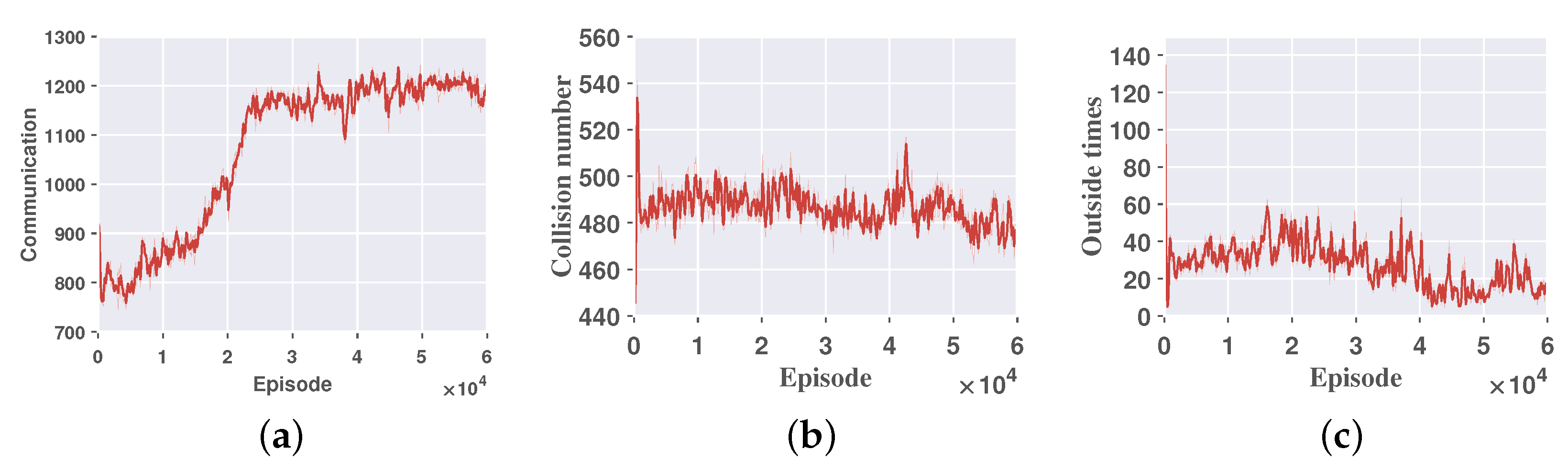
• Communication return.The communication return is the average communication quality per episode for the UGVs and is calculated based on Equation (1). The communication returns converge quickly from the initial –800 to –300 as shown by Figure 5a, which indicates that the communication quality has been improved and has stabilized in an interval.
• Collision times: The collision times are the sum of collisions between UGVs and obstacles and between drones and drones in an average round. The collision indicator converges from 540 to below 480, as shown by Figure 5b, indicating that the number of collisions has also been reduced somewhat, and since this study allows UGVs to have a certain number of collisions, the collision indicator is not the main optimization objective.
• Outside times: The outside times are the number of times the UGVs go out of bounds and run out of the environment we set. From Figure 5c, the rapid reduction in the number of times going out of bounds indicates that our research has significantly limited ineffective boundary violations, demonstrating that our study effectively operates within the designated area.

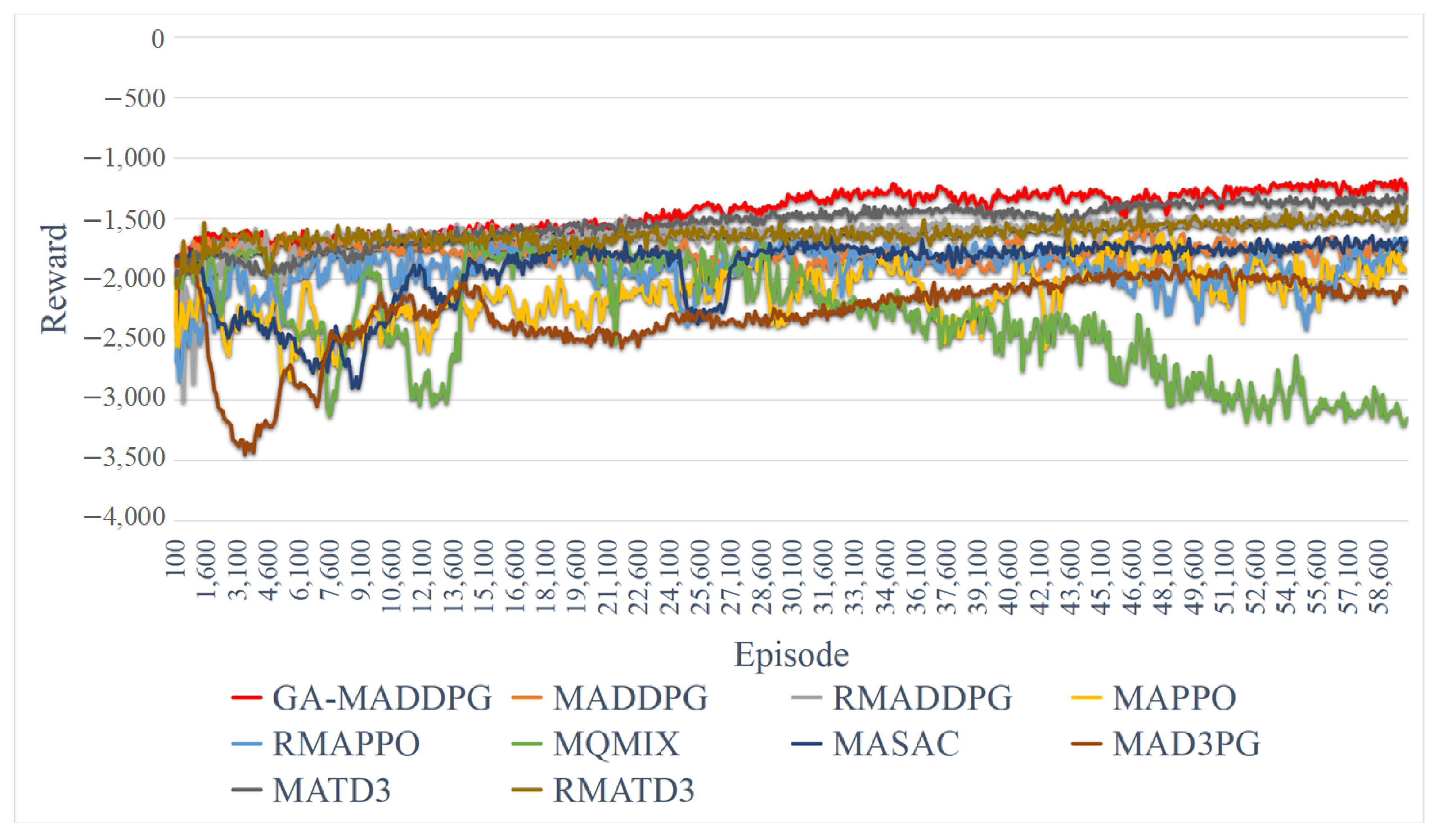
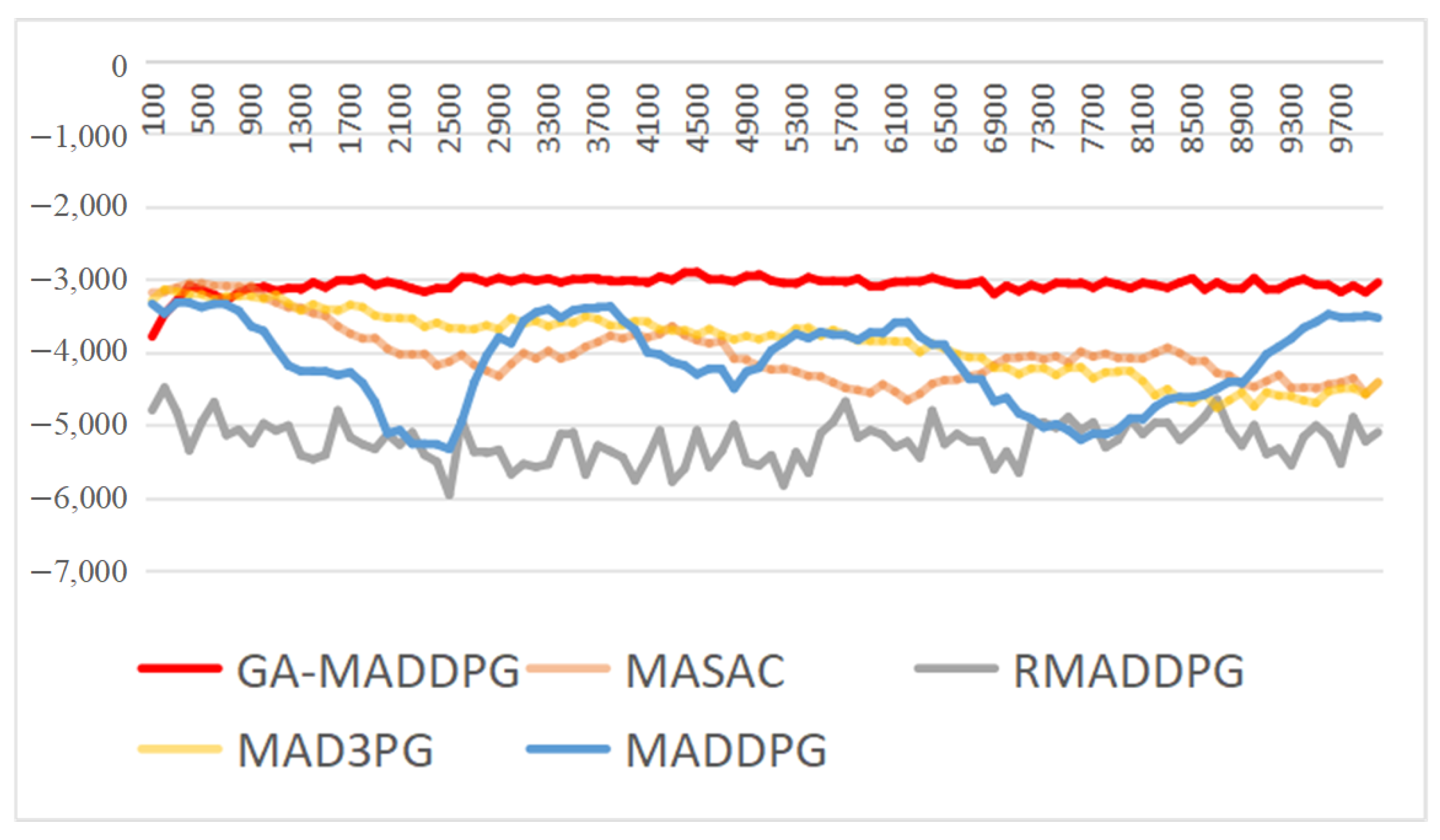
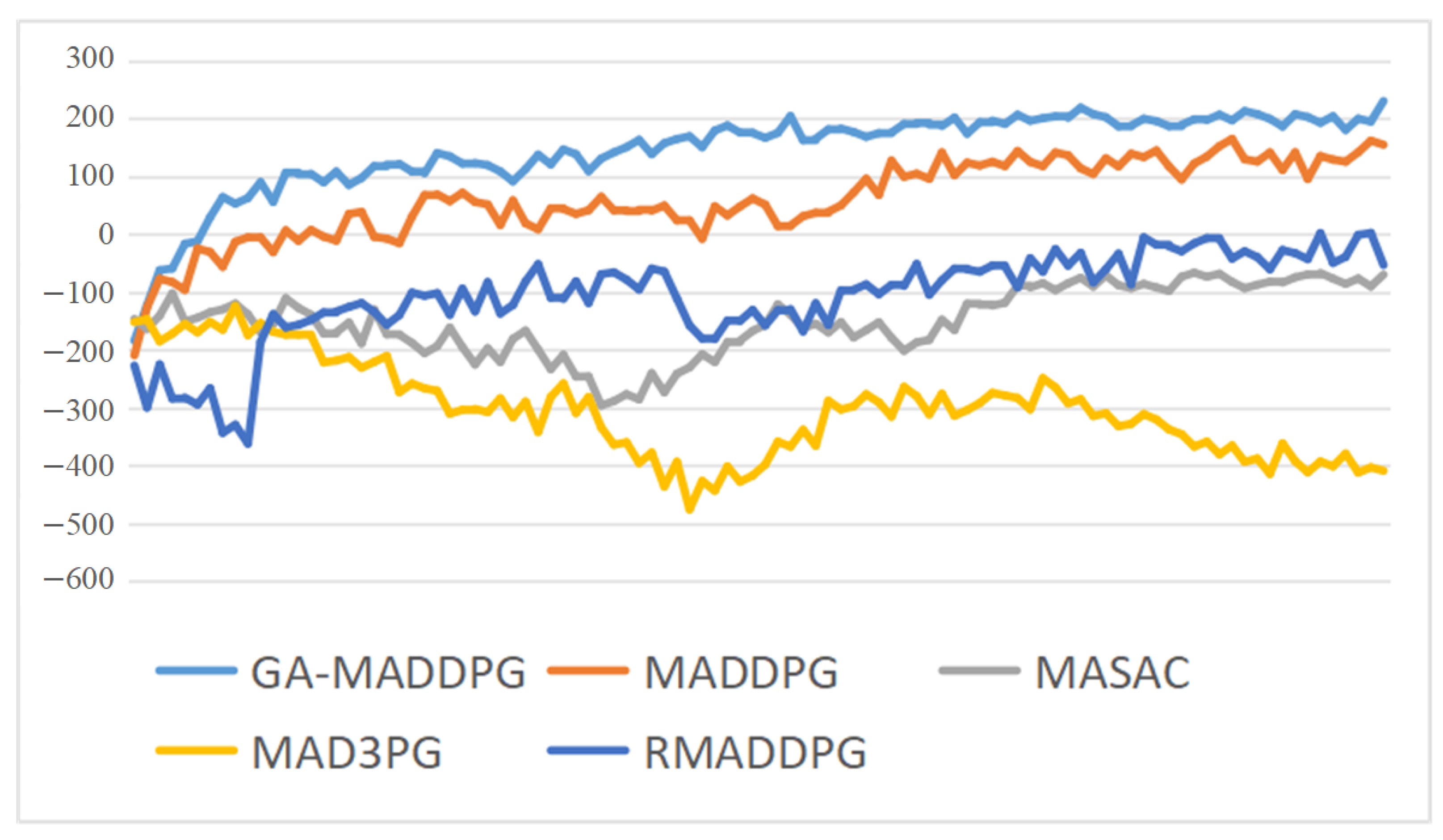
4.3. Comparative GA-MADDPG Experimentation

To compare with the suggested algorithm and determine whether the algorithm works better, we provide seven RL approaches that are thought of as baselines. The methods are MADDPG [24]: a classic multi-agent deep deterministic policy gradient, R-MADDPG [38]: a deep recurrent multi-agent actor–critic, MAPPO [39]: multi-agent proximal policy optimization, RMAPPO [39]: a deep recurrent multi-agent proximal policy optimization, MQMIX [40]: mellow–max monotonic value function factorization for deep multi-agent, MASAC [41]: a classic multi-agent soft actor–critic, MAD3PG [42]: a multi-agent deep distributional deterministic policy gradient, MATD3 [43]: the twin delayed deep deterministic policy gradient, and RMATD3 [44]: the twin delayed deep deterministic policy gradient with a deep recurrent. Notably, we replicate these baselines using the same simulation environment to guarantee the experiment is fair.

The cumulative return of the GA-MADDPG and other algorithms, which is displayed in Figure 6, indicates the experimental comparison findings and highlights the potency of GA-MADDPG algorithms. GA-MADDPG outperforms the other algorithms by achieving a considerably higher reward return of about −1200 with 60,000 episodes, reaching its convergence point. Furthermore, as shown in Figure 6, both MADDPG and R-MADDPG achieve lower rewards of around −1600 compared to GA-MADDPG, providing strong evidence for the effectiveness of our contribution: the use of GA adaptive hyperparameters allows for better jumps out of the local optima and higher rewards. As shown in Figure 6, in the specific environment we configured, neither the original MADDPG algorithm nor its variant incorporating deep recurrent networks outperforms GA-MADDPG in areas of convergence speed and final convergence outcomes: GA-MADDPG converges in about 2000 episodes, while R-MADDPG converges in about 5000 episodes, and the original algorithm MADDPG converges even worse. Of greater significance, our experimental findings reveal that MASAC, MAPPO, MAD3PG, MQMIX, and RMAPPO encounter challenges in achieving a desirable convergence state within the multi-agent cooperative environment we constructed. MASAC required approximately 25,000 episodes to converge, ultimately stabilizing at a reward value of approximately −1800. MAPPO and RMAPPO exhibited less stable convergence, with rewards fluctuating between −2000 and −2500. Meanwhile, MAD3PG’s reward converged to approximately −2100. Regarding MQMIX, its reward demonstrated initial oscillation over the first 25,000 episodes, followed by a steady decline thereafter. This further emphasizes the superiority of GA-MADDPG in terms of performance and effectiveness.

Furthermore, certain algorithms tend to converge to local optima, which further reinforces the effectiveness of our decision to adopt the MADDPG algorithm and enhance it. As depicted in Figure 6, in the initial 25,000 episodes, GA-MADDPG may succumb to local optimality. However, the incorporation of the GA mechanism enables GA-MADDPG to attain elevated rewards beyond this threshold. Notably, MAPPO and MQMIX demonstrate subpar performance, possibly due to the lack of adaptive hyperparameter updates, hindering their effective cooperation within the multi-agent environment and leading to convergence challenges. Therefore, this observation naturally demonstrates the high effectiveness of incorporating GA into multi-agent RL algorithms. By introducing GA, multi-agent algorithms can more effectively avoid falling into local optima, resulting in improved convergence speed and outcomes. And the variation of the loss calculated by Equation (21) is represented by Figure 7, from which we can see the constant convergence of the loss to near 1800, which can prove the convergence of the algorithm. During the validation process, Figure 8 displays several simulated paths of UGVs. Under optimal communication conditions, the BS UGV might remain stationary to prevent potential losses due to collisions. However, in situations with less than excellent communication, the BS UGV proactively moves to compensate for communication limitations. Additionally, statistics for the three evaluation indicators (Figure 5) show the improvement in communication return, the reduction in collision number, and the decrease in outside number as the algorithm converges. The return on communications exhibited an improvement from an initial value of −800 to −300 towards the conclusion of the experiment. Concurrently, the frequency of collisions decreased from 540 to 470, and the occurrences of external events diminished from 100 to nearly zero. This suggests that as the algorithm converges, the three evaluation metrics also reach optimality.

4.4. Generalization Experiment of GA-MADDPG

4.4.1. Simulation with Different Numbers of UGVs

To further prove the universality of the proposed GA-MADDPG algorithm in the set environment, this study also designed two other generalization experiments for the scene. The experiment set different numbers of UGVs, target points, and obstacles in the scene to determine whether the algorithm GA-MADDPG can continue to perform superiorly. It should be noted that since some baseline algorithms in Section 4.3 have performed poorly or even have difficultly converging, the generalization experiment uses four baseline algorithms that are relatively stable in Section 4.3, including MASAC, MAD3PG, MADDPG, and its variant, RMADDPG. Generalization environment 1: The number of UGVs increases to four, the number of mobile base stations is one, the number of target points increases to four, and the number of obstacles increases to seven. The significance of setting up the environment in this way is to increase the severity of the environment by increasing the number of UGVs and the number of obstacles.

From Figure 9, we can see that despite the increased complexity of the environment, the GA-MADDPG algorithm always has a higher convergence value in harsh environments and can converge to a high value well. The GA-MADDPG algorithm can maintain convergence to a reward value of −3000, while the other baseline algorithms do not perform well or even find it difficult to converge in complex environments, and the highest reward value is only around −3300. This fully demonstrates that the GA-MADDPG algorithm still has better performance than other algorithms after the environmental complexity increases.

Generalized environment 2: The number of UGVs is reduced to two, the number of mobile base stations is one, the number of target points is reduced to two, and the number of obstacles is reduced to three. The significance of setting up the environment in this way is to improve the simplicity of the environment by simplifying the number of UGVs and obstacles so that the UGV can complete the goal with a greater reward.

As can be seen from Figure 10, the rewards of most algorithms show a good upward trend. This is because the generalized environment uses a simpler three UGVs (including a UGV base station), three obstacles, and two target points. The algorithm performs better in a simple environment and convergence is easier than for the generalized environment. As the number of vehicles decreases, the number of collisions and out-of-bounds also decrease accordingly. It should be noted that since the communication environment parameters remain unchanged, the reward value of the overall algorithm is positive, which is normal. From Figure 10, it can be seen that in this generalized environment, the reward of the GA-MADDPG algorithm always remains ahead, both in terms of convergence speed and final convergence value, which are much higher than for the other algorithms, and the final reward value can converge to about 200. As a basic algorithm, MADDPG also has a higher convergence value of about 150. This fully demonstrates that the GA-MADDPG algorithm can also perform well in a simple environment.

It can be seen from Figure 9 and Figure 10 that in the experimental environments with two different parameter settings, despite changes in the number of UGVs, the number of target points, and the number of obstacles, the GA-MADDPG algorithm can still perform better than the other algorithms, which fully demonstrates the robustness of the GA-MADDPG algorithm and its universality to environmental scenarios.

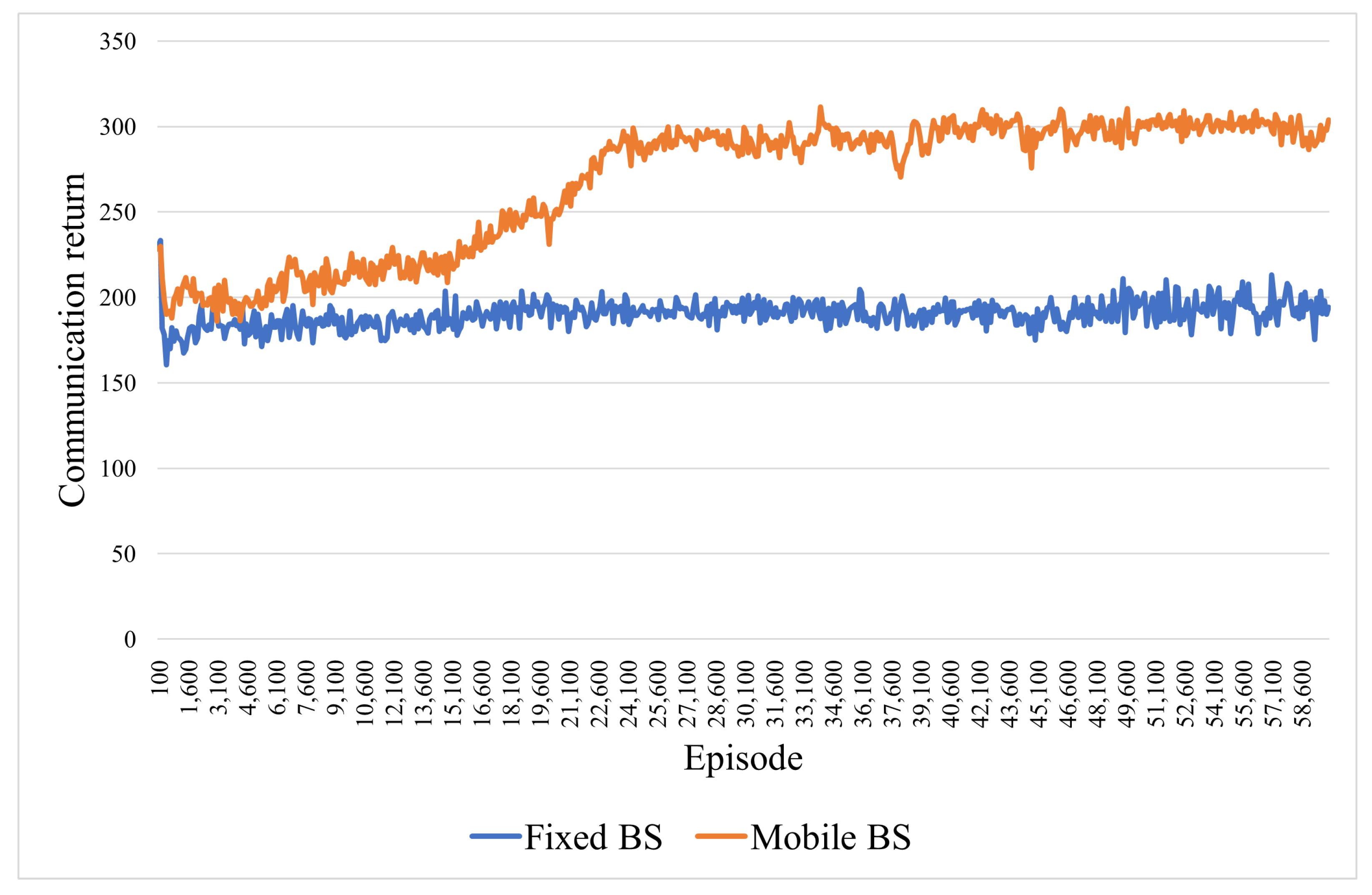
4.4.2. Experiments on the Effectiveness of the Mobile BS

The previous subsections prove the stability and convergence of our proposed algorithm. Also, the last section proves that our proposed algorithm is superior in the same scenario. To better demonstrate the effectiveness of the mobile base station proposed in this paper, we add an extra experiment: only changing the mobile BS to a fixed BS but using the same algorithm.

We use the communication return as an evaluation metric, and the communication return with a mobile base station is better than that of the fixed base station from the beginning of training, as shown by Figure 11. The communication return of a single UGV can eventually converge to around 300, while that of the fixed base station hovers around 200 feet, which fully proves the effectiveness of our proposed mobile base station.

5. Conclusions

In this article, a cooperative system for multi-UGV cooperative navigation within a communication coverage area is proposed. The system is formulated as an MDP to determine an optimal navigation policy for the UGVs, with the aim of maximizing the total reward. In contrast to prior studies focusing on fixed coverage-aware navigation, this paper introduces a novel approach by incorporating a mobile BS into the multi-intelligent-body algorithm. This innovation aims to enhance communication coverage and expand the solution space available for intelligent agents. To mitigate the risk of local optima, this study introduces a GA hyperparameter adaptive updating mechanism to address the multi-UGV navigation problem. We coin the term GA-MADDPG to refer to this novel RL algorithm. The simulation results demonstrate that GA-MADDPG exhibits favorable performance, convergence rates, and effectiveness compared to other RL algorithms.

In our future research, we would like to address the following points: (1) To enhance model realism, one can combine a traditional PID control with multi-agent RL and further optimize the navigation policy by taking control of the machine operation. (2) One can try to use a new architecture to learn policies, such as by using LSTM (long short-term memory) and the transformer architecture. LSTM can solve the problem of gradient vanishing and gradient explosion during the training of long sequences; the advantage of the transformer architecture is that its attention layer can learn a sequence of actions very well.

References

1. Afzali, S.R.; Shoaran, M.; Karimian, G. A Modified Convergence DDPG Algorithm for Robotic Manipulation. Neural Process. Lett. 2023, 55, 11637–11652. [Google Scholar] [CrossRef]
2. Chai, R.; Niu, H.; Carrasco, J.; Arvin, F.; Yin, H.; Lennox, B. Design and experimental validation of deep reinforcement learning-based fast trajectory planning and control for mobile robot in unknown environment. IEEE Trans. Neural Netw. Learn. Syst. 2022, 35, 5778–5792. [Google Scholar] [CrossRef]
3. Dong, X.; Wang, Q.; Yu, J.; Lü, J.; Ren, Z. Neuroadaptive Output Formation Tracking for Heterogeneous Nonlinear Multiagent Systems with Multiple Nonidentical Leaders. IEEE Trans. Neural Netw. Learn. Syst. 2022, 35, 3702–3712. [Google Scholar] [CrossRef]
4. Wang, Y.; Zhao, C.; Liang, J.; Wen, M.; Yue, Y.; Wang, D. Integrated Localization and Planning for Cruise Control of UGV Platoons in Infrastructure-Free Environments. IEEE Trans. Intell. Transp. Syst. 2023, 24, 10804–10817. [Google Scholar] [CrossRef]
5. Tran, V.P.; Perera, A.; Garratt, M.A.; Kasmarik, K.; Anavatti, S.G. Coverage Path Planning with Budget Constraints for Multiple Unmanned Ground Vehicles. IEEE Trans. Intell. Transp. Syst. 2023, 24, 12506–12522. [Google Scholar] [CrossRef]
6. Wu, Y.; Li, Y.; Li, W.; Li, H.; Lu, R. Robust Lidar-Based Localization Scheme for Unmanned Ground Vehicle via Multisensor Fusion. IEEE Trans. Neural Netw. Learn. Syst. 2021, 32, 5633–5643. [Google Scholar] [CrossRef]
7. Zhang, W.; Zuo, Z.; Wang, Y. Networked multiagent systems: Antagonistic interaction, constraint, and its application. IEEE Trans. Neural Netw. Learn. Syst. 2021, 33, 3690–3699. [Google Scholar] [CrossRef] [PubMed]
8. Chen, D.; Weng, J.; Huang, F.; Zhou, J.; Mao, Y.; Liu, X. Heuristic Monte Carlo algorithm for unmanned ground vehicles realtime localization and mapping. IEEE Trans. Veh. Technol. 2020, 69, 10642–10655. [Google Scholar] [CrossRef]
9. Unlu, H.U.; Patel, N.; Krishnamurthy, P.; Khorrami, F. Sliding-window temporal attention based deep learning system for robust sensor modality fusion for UGV navigation. IEEE Robot. Autom. Lett. 2019, 4, 4216–4223. [Google Scholar] [CrossRef]
10. Lyu, X.; Hu, B.; Wang, Z.; Gao, D.; Li, K.; Chang, L. A SINS/GNSS/VDM integrated navigation fault-tolerant mechanism based on adaptive information sharing factor. IEEE Trans. Instrum. Meas. 2022, 71, 1–13. [Google Scholar] [CrossRef]
11. Sun, C.; Ye, M.; Hu, G. Distributed optimization for two types of heterogeneous multiagent systems. IEEE Trans. Neural Netw. Learn. Syst. 2020, 32, 1314–1324. [Google Scholar] [CrossRef]
12. Shan, Y.; Fu, Y.; Chen, X.; Lin, H.; Lin, J.; Huang, K. LiDAR based Traversable Regions Identification Method for Off-road UGV Driving. IEEE Trans. Intell. Veh. 2023, 9, 3544–3557. [Google Scholar] [CrossRef]
13. Garaffa, L.C.; Basso, M.; Konzen, A.A.; de Freitas, E.P. Reinforcement learning for mobile robotics exploration: A survey. IEEE Trans. Neural Netw. Learn. Syst. 2021, 34, 3796–3810. [Google Scholar] [CrossRef]
14. Huang, C.Q.; Jiang, F.; Huang, Q.H.; Wang, X.Z.; Han, Z.M.; Huang, W.Y. Dual-graph attention convolution network for 3-D point cloud classification. IEEE Trans. Neural Netw. Learn. Syst. 2022, 35, 4813–4825. [Google Scholar] [CrossRef]
15. Nguyen, H.T.; Garratt, M.; Bui, L.T.; Abbass, H. Supervised deep actor network for imitation learning in a ground-air UAV-UGVs coordination task. In Proceedings of the 2017 IEEE Symposium Series on Computational Intelligence (SSCI), Honolulu, HI, USA, 27 November–1 December 2017; IEEE: Piscataway, NJ, USA, 2017; pp. 1–8. [Google Scholar]
16. Han, Z.; Yang, Y.; Wang, W.; Zhou, L.; Gadekallu, T.R.; Alazab, M.; Gope, P.; Su, C. RSSI Map-Based Trajectory Design for UGV Against Malicious Radio Source: A Reinforcement Learning Approach. IEEE Trans. Intell. Transp. Syst. 2022, 24, 4641–4650. [Google Scholar] [CrossRef]
17. Feng, Z.; Huang, M.; Wu, Y.; Wu, D.; Cao, J.; Korovin, I.; Gorbachev, S.; Gorbacheva, N. Approximating Nash equilibrium for anti-UAV jamming Markov game using a novel event-triggered multi-agent reinforcement learning. Neural Netw. 2023, 161, 330–342. [Google Scholar] [CrossRef]
18. Huang, X.; Deng, H.; Zhang, W.; Song, R.; Li, Y. Towards multi-modal perception-based navigation: A deep reinforcement learning method. IEEE Robot. Autom. Lett. 2021, 6, 4986–4993. [Google Scholar] [CrossRef]
19. Wu, S.; Xu, W.; Wang, F.; Li, G.; Pan, M. Distributed federated deep reinforcement learning based trajectory optimization for air-ground cooperative emergency networks. IEEE Trans. Veh. Technol. 2022, 71, 9107–9112. [Google Scholar] [CrossRef]
20. Watkins, C.J.; Dayan, P. Q-learning. Mach. Learn. 1992, 8, 279–292. [Google Scholar] [CrossRef]
21. Tran, T.H.; Nguyen, M.T.; Kwok, N.M.; Ha, Q.P.; Fang, G. Sliding mode-PID approach for robust low-level control of a UGV. In Proceedings of the 2006 IEEE International Conference on Automation Science and Engineering, Shanghai, China, 8–10 October 2006; IEEE: Piscataway, NJ, USA, 2006; pp. 672–677. [Google Scholar]
22. Schaul, T.; Quan, J.; Antonoglou, I.; Silver, D. Prioritized experience replay. arXiv 2015, arXiv:1511.05952. [Google Scholar]
23. Sutton, R.S.; Barto, A.G. Reinforcement Learning: An Introduction. IEEE Trans. Neural Netw. 1998, 9, 1054. [Google Scholar] [CrossRef]
24. Lowe, R.; Wu, Y.I.; Tamar, A.; Harb, J.; Pieter Abbeel, O.; Mordatch, I. Multi-agent actor-critic for mixed cooperative-competitive environments. arXiv 2017, arXiv:1706.02275. [Google Scholar]
25. Mirjalili, S.; Mirjalili, S. Genetic algorithm. Evolutionary Algorithms and Neural Networks: Theory and Applications; Springer: Berlin/Heidelberg, Germany, 2019; pp. 43–55. [Google Scholar]
26. Sehgal, A.; La, H.; Louis, S.; Nguyen, H. Deep reinforcement learning using genetic algorithm for parameter optimization. In Proceedings of the 2019 Third IEEE International Conference on Robotic Computing (IRC), Naples, Italy, 25–27 February 2019; IEEE: Piscataway, NJ, USA, 2019; pp. 596–601. [Google Scholar]
27. Chen, R.; Yang, B.; Li, S.; Wang, S. A self-learning genetic algorithm based on reinforcement learning for flexible job-shop scheduling problem. Comput. Ind. Eng. 2020, 149, 106778. [Google Scholar] [CrossRef]
28. Alipour, M.M.; Razavi, S.N.; Feizi Derakhshi, M.R.; Balafar, M.A. A hybrid algorithm using a genetic algorithm and multiagent reinforcement learning heuristic to solve the traveling salesman problem. Neural Comput. Appl. 2018, 30, 2935–2951. [Google Scholar] [CrossRef]
29. Liu, Z.; Chen, B.; Zhou, H.; Koushik, G.; Hebert, M.; Zhao, D. Mapper: Multi-agent path planning with evolutionary reinforcement learning in mixed dynamic environments. In Proceedings of the 2020 IEEE/RSJ International Conference on Intelligent Robots and Systems (IROS), Las Vegas, NV, USA, 25–29 October 2020; IEEE: Piscataway, NJ, USA, 2020; pp. 11748–11754. [Google Scholar]
30. Huang, M.; Lin, X.; Feng, Z.; Wu, D.; Shi, Z. A multi-agent decision approach for optimal energy allocation in microgrid system. Electr. Power Syst. Res. 2023, 221, 109399. [Google Scholar] [CrossRef]
31. Qiu, C.; Hu, Y.; Chen, Y.; Zeng, B. Deep deterministic policy gradient (DDPG)-based energy harvesting wireless communications. IEEE Internet Things J. 2019, 6, 8577–8588. [Google Scholar] [CrossRef]
32. Littman, M.L. Markov games as framework for multi-agent reinforcement learning. In Proceedings of the Proc International Conference on Machine Learning, New Brunswick, NJ, USA, 10–13 July 1994; pp. 157–163. [Google Scholar]
33. Feng, Z.; Huang, M.; Wu, D.; Wu, E.Q.; Yuen, C. Multi-Agent Reinforcement Learning with Policy Clipping and Average Evaluation for UAV-Assisted Communication Markov Game. IEEE Trans. Intell. Transp. Syst. 2023, 24, 14281–14293. [Google Scholar] [CrossRef]
34. Liu, H.; Zong, Z.; Li, Y.; Jin, D. NeuroCrossover: An intelligent genetic locus selection scheme for genetic algorithm using reinforcement learning. Appl. Soft Comput. 2023, 146, 110680. [Google Scholar] [CrossRef]
35. Köksal Ahmed, E.; Li, Z.; Veeravalli, B.; Ren, S. Reinforcement learning-enabled genetic algorithm for school bus scheduling. J. Intell. Transp. Syst. 2022, 26, 269–283. [Google Scholar] [CrossRef]
36. Chen, Q.; Huang, M.; Xu, Q.; Wang, H.; Wang, J. Reinforcement Learning-Based Genetic Algorithm in Optimizing Multidimensional Data Discretization Scheme. Math. Probl. Eng. 2020, 2020, 1698323. [Google Scholar] [CrossRef]
37. Yang, J.; Sun, Z.; Hu, W.; Steinmeister, L. Joint control of manufacturing and onsite microgrid system via novel neural-network integrated reinforcement learning algorithms. Appl. Energy 2022, 315, 118982. [Google Scholar] [CrossRef]
38. Shi, H.; Liu, G.; Zhang, K.; Zhou, Z.; Wang, J. MARL Sim2real Transfer: Merging Physical Reality with Digital Virtuality in Metaverse. IEEE Trans. Syst. Man Cybern. Syst. 2023, 53, 2107–2117. [Google Scholar] [CrossRef]
39. Yu, C.; Velu, A.; Vinitsky, E.; Gao, J.; Wang, Y.; Bayen, A.; Wu, Y. The surprising effectiveness of ppo in cooperative multi-agent games. Adv. Neural Inf. Process. Syst. 2022, 35, 24611–24624. [Google Scholar]
40. Rashid, T.; Farquhar, G.; Peng, B.; Whiteson, S. Weighted qmix: Expanding monotonic value function factorisation for deep multi-agent reinforcement learning. Adv. Neural Inf. Process. Syst. 2020, 33, 10199–10210. [Google Scholar]
41. Wu, T.; Wang, J.; Lu, X.; Du, Y. AC/DC hybrid distribution network reconfiguration with microgrid formation using multi-agent soft actor-critic. Appl. Energy 2022, 307, 118189. [Google Scholar] [CrossRef]
42. Yan, C.; Xiang, X.; Wang, C.; Li, F.; Wang, X.; Xu, X.; Shen, L. PASCAL: PopulAtion-Specific Curriculum-based MADRL for collision-free flocking with large-scale fixed-wing UAV swarms. Aerosp. Sci. Technol. 2023, 133, 108091. [Google Scholar] [CrossRef]
43. Ackermann, J.J.; Gabler, V.; Osa, T.; Sugiyama, M. Reducing Overestimation Bias in Multi-Agent Domains Using Double Centralized Critics. arXiv 2019, arXiv:1910.01465. [Google Scholar]
44. Xing, X.; Zhou, Z.; Li, Y.; Xiao, B.; Xun, Y. Multi-UAV Adaptive Cooperative Formation Trajectory Planning Based on an Improved MATD3 Algorithm of Deep Reinforcement Learning. IEEE Trans. Veh. Technol. 2024. [Google Scholar] [CrossRef]
Figure 1. Schematic diagram of the collaboration of a swarm of UGVs in a communication-enabled environment. (a) 3D urban environment. (b) Top view of the visualized communication environment.
Electronics 13 03028 g001
Figure 2. The results of changing communication in the environment as the mobile BS moves. The red areas indicate better communication, whereas the blue areas indicate poorer communication, Brown circles represent the mobile BS, blue circles represent UGVs, black circles represent obstacles, and red circles represent target points. This movement aims to enhance communication quality for the UGVs.
Electronics 13 03028 g002
Figure 3. Detailed diagram of the GA-MADDPG algorithm.
Electronics 13 03028 g003
Figure 4. Plan view of base station model distribution.
Electronics 13 03028 g004
Figure 5. Three evaluation indicators for UGV navigation. (a) Communication return. (b) Collision number. (c) Outside times.
Electronics 13 03028 g005
Figure 6. Average cost of the GA-MADDPG and other advanced algorithms.
Electronics 13 03028 g006
Figure 7. Evolution of loss function.
Electronics 13 03028 g007
Figure 8. Some UGV path maps based on GA-MADDPG.
Electronics 13 03028 g008
Figure 9. Average cost comparison of generalization environment 1.
Electronics 13 03028 g009
Figure 10. Average cost comparison of generalization environment 2.
Electronics 13 03028 g010
Figure 11. Comparison of communication returns between mobile BS and fixed BS.
Electronics 13 03028 g011