A Prosumer Hydro Plant Network as a Sustainable Distributed Energy Depot

Abstract

The shortage of efficient, low-cost storage depots inhibits the large-scale adoption of volatile-by-nature, renewable sources of energy (RSEs). In this paper, we outline how to utilize prosumer-owned hydro plants of a few to several kW as a distributed, short-term energy storage solution that is deployable with little investment and a low operational expenditure. The proposed solution is a system of interconnected hydro depots with an active water-flow control algorithm that reduces the grid’s load variability and benefits prosumers. According to the tests conducted, prosumer revenue grows from several percent to over 30 percent, depending on weather conditions, in comparison to the free-flow case. In turn, the cushioning effect of the distributed energy buffer balances the fluctuations introduced by other RSEs, e.g., photovoltaic- or wind-based ones. Hence, while benefitting the involved parties, it also facilitates the inclusion of RSEs within the power distribution system.

1. Introduction

Electrical energy is considered the bloodstream of today’s society. Electricity use in homes, industry, transportation, and building cooling and heating results in increased demand on a daily basis. Meanwhile, energy generation continues to be expensive, both from an environmental and an economic point of view. Global pollution, the growing cost of fossil fuels, and political pressure are just a few factors that encourage energy production from renewable sources (RSEs), e.g., the sun, wind, waves, geothermal energy, and water movement [1]. Unfortunately, the amount of energy retrieved from RSEs depends heavily on temporal weather conditions. RSEs provide inexpensive energy either at random hours (wind) or around noon (solar, mostly photovoltaic (PV)). In contrast, the demand remains at a similar level until the evening, as illustrated in Figure 1. Hence, costly, fossil-fuel-sourced plants need to be engaged in the evenings, but their activity should be constrained in favor of RSEs if the sun or wind is available. Moreover, energy generation from traditional thermal plants cannot be constrained too much due to technological factors. As a result of market dynamics, energy prices are set low (or even negative) at certain times to then reach a higher order of magnitude a few hours later, resembling the ‘duck curve’ depicted in Figure 2, which shows the initial days of July 2023 in the Polish energy market. In the interest of all stakeholders, this disparity should be reduced.

A self-imposed solution to the producer–consumer disparity is to store surplus energy when it is cheap for a later time when costly sources are incorporated. Unfortunately, today’s technology does not permit executing this on a larger scale [2]. For instance, pumped hydro plants in Poland can deliver, at most, 5% of the overall power demand, and the battery depots only deliver 1% at most. Both of these traditional methods, as well as prospective hydrogen-based systems, are expensive to deploy and maintain. The low durability of electromechanical batteries further restricts a good return on one’s investment. Hence, seeking a new, low-CAPEX (capital expenditures) and low-OPEX (operational expenditures) option for energy storage is desirable.

Recently, a substantial change in the electricity market has been observed. Traditional, large power plants are being supplemented by small-scale facilities installed by citizens on their own premises. These citizens are electricity consumers during certain hours of the day and producers at other times and are thus called prosumers. On the one hand, the popularity of prosumer installations advances the adoption of RSEs; on the other hand, it threatens the stability of the energy supply system by forcing extreme load changes on traditional plants.

This study contributes to the aforementioned challenges in the following ways:

• We propose engaging prosumer hydro plants with a peak power in the range of a few kW in order to form a distributed energy depot;
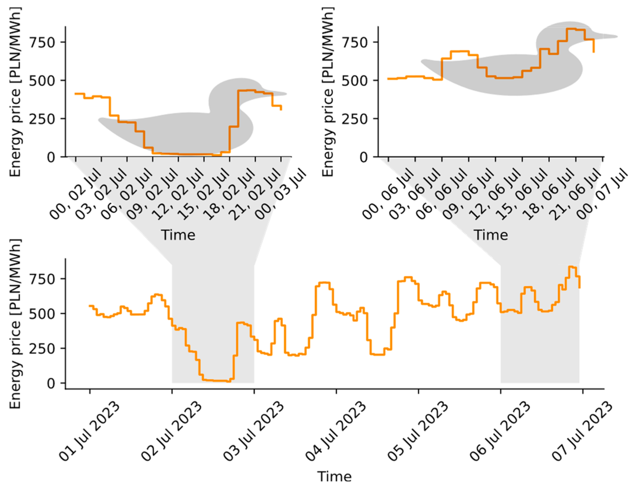
• We design an active control scheme, which allows for both increasing the revenue of the plant owners and reducing the load variability imposed on legacy thermal plants (“beheading the duck” [3]), thus achieving a win–win solution;
• Contrary to the typical approach, which focuses on a single hybrid generator, e.g., [4], we show how to co-ordinate a network of plants for a safe and efficient distributed system operation.

Figure 1. Energy generation from principal RSEs and predicted energy demands in Poland for 1–6 July 2023 (1 July was a Saturday [5]).

Figure 1. Energy generation from principal RSEs and predicted energy demands in Poland for 1–6 July 2023 (1 July was a Saturday [5]).

Figure 2. Fluctuation in next-day market energy prices [PLN/MWh] in the Polish market over 1–6 July 2023, following the ‘duck curve’ [5].

Figure 2. Fluctuation in next-day market energy prices [PLN/MWh] in the Polish market over 1–6 July 2023, following the ‘duck curve’ [5].

The remainder of the paper is organized as follows. In Section 2, the traditional methods of hydro plant control are discussed. In Section 3, we elaborate on the differences between conventional and prosumer plants. In Section 4, a discrete-time dynamic model of water flow in a multi-hydro plant system is constructed, and a procedure to optimize its operation is described. In Section 5, we evaluate the algorithm’s performance for a broad spectrum of test data. Then, we discuss the implementation considerations in Section 6. Finally, conclusions are drawn in Section 7.

2. Control of Hydro Plants

In the literature, hydro plants (HPs) are classified as normal (>100 MW), medium (<100 MW), small (<15 MW), mini (<1 MW), micro (<100 kW), or pico (<5 kW) HPs, although the actual values vary by region [6,7]. Most of the research concentrates on small, medium, and normal HPs, which play a pronounced role in electricity supply. In this paper, owing to their significance for prosumers, micro- and pico-HPs are investigated. They encompass numerous formerly abandoned mills with small artificial ponds, swamps, and other natural formations, commonly known as run-of-river HPs [8,9], thus requiring insignificant capital expenditures for deployment. For example, currently, in Poland, less than 5% of possible installations are used for energy production [10]. Moreover, numerous online service publications show that pico-HPs can be easily deployed without specialized equipment [11]. Thus, the target area of the study conducted in this work is important. Of course, a single prosumer depot is not a game-changer. However, a revenue-oriented, optimally scheduled set of prosumer HPs may constitute an efficient energy storage system resistant to perturbances with low operational costs. In fact, similar circumstances led to the popularity of PV installations, which have become a common element of the present landscape.

However, there is a fundamental difference between PV and HP installations. The PV ones are mutually independent, whereas the proper operation of an HP depends on all the stations upstream being linked in a cascade. In the past, the scheduling of the operation of a cascade of HPs has been investigated as a case study [12] rather than as a networked system subjected to a control action, i.e., each plant was adjusted manually without enforcing a common framework. While a suitable scheduling plan can be defined in this way, it may not account for the optimal operating conditions or pose a risk in terms of drought/flood protection. Other approaches consider simplified models, reducing the cascade to a single-plant case [4], where the dams are at a close distance [8,13] or located on one river but not on its tributaries [9,14]. A solution conceptually closest to the one discussed here has been proposed in [13], albeit it targets large, concentrated installations and not the distributed HPs under prosumer management.

Technically, the steering of energy production at a hydro plant is not an intricate process. By raising the weirs, one constrains the water flow and, by lowering them, one increases energy generation. However, establishing the correct sequence of raising and lowering the weirs is far from obvious. Usually, the scheduling strategy is categorized as long-term (1–5 years), mid-term (3–18 months), and short-term (2–14 days) [15]. Nevertheless, in the case of prosumer HPs, such strategies are of limited usefulness due to the small volume of the ponds. In the considered case, a meaningful scheduling strategy should span the range of a few hours or, at most, one day. Moreover, it should focus on decreasing the generation–consumption imbalance in the evenings and mornings (Figure 2) or, equivalently, take advantage of the fluctuating market prices resulting from the disparity between forecasted and actual demands [16] (Figure 1).

The optimal scheduling of the HP water release problem has been investigated for a long time ([15,17] and the references therein). However, in those studies, HPs were examined only in the context of either flood/drought protection or power generation. Here, a third role of HPs is explored, i.e., the potential to provide an energy depot [2]. Instead of focusing just on the amount of generated electricity, HPs may constrain the river flow when the energy is cheap and increase it when the price grows, thus creating an efficient energy buffer. The overall amount of the generated energy will remain the same, but the HP owner revenue will grow by embracing the short-time changes in the price profile. Simultaneously, the fluctuation of energy generation from the traditional thermal plants decreases. A similar idea has been explored in [18], but it is destined for large installations, not the prosumer ones considered in this work.

3. Prosumer Hydro Plants

Not all RSEs are sensitive to the influence of weather fluctuations, e.g., geothermal, tide-based, or large, costly hydro HPs [19]. Here, the focus is on small, flexible installations, i.e., micro- [6] and pico-HPs [20]. They are typically deployed as run-on-river installations [8,21], i.e., without large dams and reservoirs, and thus they do not have significant expenditures or intrusion into the environment [21]. As opposed to larger HPs, which are not affected by local atmospheric conditions since the amount of water over the predictions is negligible compared to the reservoir volume, the limited storage space of micro- and pico-reservoirs does make them susceptible to weather variability. For instance, a local storm can promptly fill up the pond near one micro-HP while a nearby one simultaneously has sunny and dry conditions. Today, precipitation forecasting is not precise enough to deal with such situations. The water runoff models are not accurate either [22]. Therefore, when the weather is unstable, the plant schedule has to be recomputed frequently to adjust the system to the most recent circumstances or the price variability in a real-time, balancing market [16]. Contrary to the commonly used numerical optimization approaches, the algorithm presented in this manuscript takes a fraction of a second to execute, even on a low-end device.

A set of HPs uses the water from upstream plants and tributaries. Hence, improper control may breed a flood. Therefore, it is mandatory to synchronize the HP operation, explicitly taking into account diverse factors:

(1)

Geographical factor—the distance between the plants and the ensuing delay of water reflow;

(2)

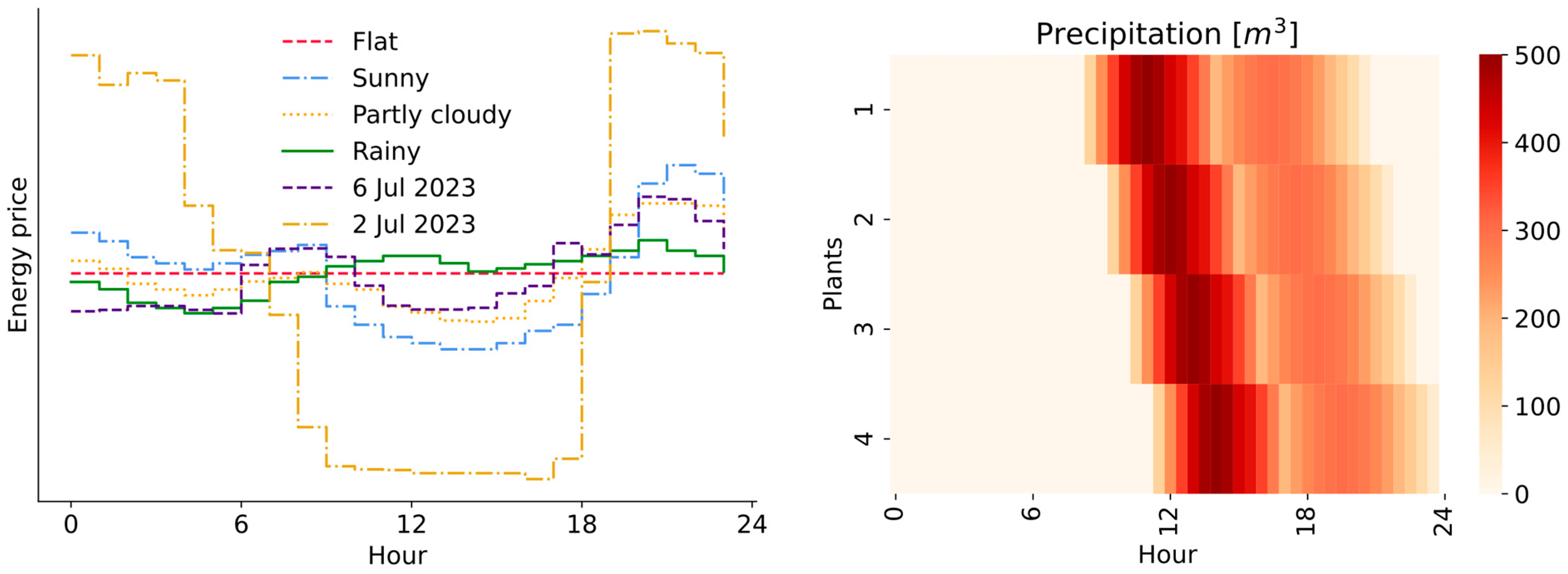
Weather-related factor—the predicted precipitation level and uncertainty level;

(3)

Application-oriented factor—the use of the HP cascade as a distributed energy depot combined with the common function of power generation.

Usually, the control schedule is established using numerical optimization procedures, incorporating artificial intelligence techniques to tackle the computational burden [15,17,21,22,23,24,25,26,27,28,29]. However, these procedures exhibit robustness issues in the considered application area, even in relatively simple cases [29]. Moreover, the large amount of time that one needs to arrive at a solution (using reasonable computing resources) contradicts the need for plan adaptability, i.e., introducing changes to the control schedule when the weather is unstable or a malfunction occurs.

To capture factors (1)–(3), information about different delays in the water flows on the links connecting the reservoirs is explicitly incorporated into the dynamical model constructed in this work. Using the system’s dynamical representation, an optimization problem is stated. It may be solved analytically if saturation is absent [30]. In contrast, here, the natural constraints are embedded in the algorithmic solution. This proposal brings benefits not only to prosumers by increasing their economic gain but also to the power grid operators by reducing the load variation for the standard power plants.

4. System Model

Usually, HP modeling concentrates on the optimization of the work of generators, ignoring the supply system [23]. Here, the generator is considered a black box, and the focus is placed on the connected HPs as a water supply system. A key point to consider in a water reflow system is the non-negligible time between issuing the control action at one reservoir before it influences the water level at a downstream one. Therefore, as opposed to the earlier models of storage networks, e.g., [31], in the approach advocated here, the control principles from time-delay storage systems [32,33] will be applied. However, the models proposed in [32,33] assume continuous-time control adjustment, which is challenging to realize in a water control system owing to the specifics of the mechanical components steering the dam weirs. The model in this work explicitly covers the effects of a finite sample time and will be constructed directly in the discrete-time domain.

4.1. Single-Plant Depot

Let us consider the model of a single HP as a constituent element of the system illustrated in Figure 3. The water budget dynamics at the plant may be described via the recursive relation

$$s_j(k+1)=s_j(k)-f_j(k)+{\displaystyle \sum _{\begin{array}{l}i\in plants \\ upstream\end{array}}{f}_i(k-T_{ij})}+r_j(k),$$

(1)

where

• k ∈ [1, m] is a time instant and m is a scheduling horizon;
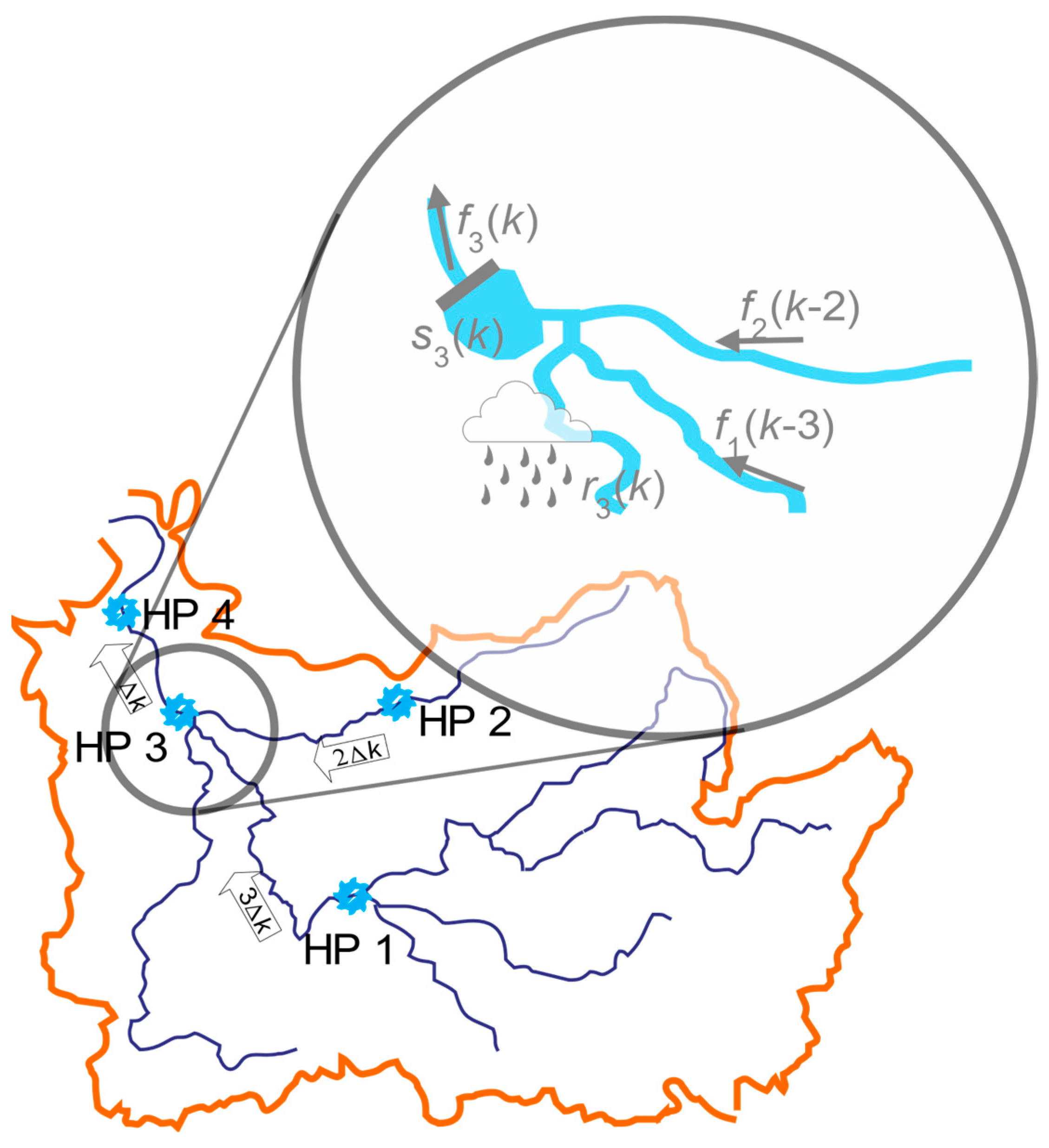
• s_j(k) is the amount of water stored in the reservoir near plant j (in Figure 3, plant j = 3 is shown in an enlarged view); s_j(k) encompasses hydroengineering construction as well as nearby swamps and similar areas;
• f_j(k) is the amount of water used to drive the power generators installed at dam j in the time between instants k and k + 1;
• r_j(k) is the supply from external hydrological sources like rain (and its runoff), melting snow, uncontrolled tributaries, and vaporization. The r_j(k) values can be obtained from the weather forecast and hydrological models within the planning horizon of m periods. r_j(k) may be positive (prevalence of precipitation) or negative (prevalence of vaporization). r_j(k) is assumed to be known in the model. When the true value of r_j(k) differs from the forecast, the algorithm is run again, which does not involve complex computations, as discussed in Section 4.3.

The tributaries supply the reservoir with the water previously used by the plants upstream. The water from upstream plant i arrives at plant j with T_ij > 0 delay. The period length Δk, i.e., the time between instants k and k + 1, can be selected arbitrarily, but according to the pace of price changes, it is reasonable to choose 1 h down to 15 min, depending on local regulations. Similarly, the planning horizon m may cover a 24 h window of known energy prices (the next-day market). The initial flow f_j(k ≤ 0) and the initial water level s_j(0) are assumed to be known. The terminal condition s_j(m) can be selected arbitrarily.

The income from the plant obtained in one period may be calculated as

$$J_j(k)={\eta }_j{p}_j(k)f_j(k)\Delta k,$$

(2)

where

• p_j(k) is the energy price at instant k. The fact that all the HPs are connected to the same system does not induce the same price profile for each plant j. The owners may have a contract with different companies, use different tariffs, or have different consumption patterns themselves;
• η_j is the efficiency of power generators, incorporating the impact of the dam height. For the prosumer generators in the lowlands, the flow of 1 m³/s corresponds to the power generation of 5–7 kW.

4.2. Multi-Plant Depot

Similar to PV, as the number of HPs grow, their impact on the grid increases. A collection of pico- and micro-HPs may constitute a large, distributed energy depot.

In the case of n power plants in the same river basin, the model variables are grouped into vectors:

$$s(k)=\left[\begin{array}{c}{s}_1(k)\\ s_2(k)\\ ⋮\\ s_n(k)\end{array}\right], f(k)=\left[\begin{array}{c}{f}_1(k)\\ f_2(k)\\ ⋮\\ f_n(k)\end{array}\right], r(k)=\left[\begin{array}{c}{r}_1(k)\\ r_2(k)\\ ⋮\\ r_n(k)\end{array}\right],$$

(3)

where s(k) is the vector of reservoir water level, f(k) is the vector of water volumes in inter-reservoir flows, and r(k) is the vector of water volumes from exogenous sources, respectively.

Derived from (1), the networked system dynamics are described by

$$s(k+1)=s(k)+{\displaystyle \sum _{t=0}^T{\Theta }_{t}f(k-t)}+r(k),$$

(4)

where T is the maximum delay, and matrices Θ_t group the information about the geographical topology and flow delays. ${\Theta }_t={\left[{\theta }_{ij}\right]}_{n\times n}$, with θ_ij = 1, if the flow from reservoir j reaches reservoir i with delay t, and otherwise, it is 0. Θ₀ describes the outflow from the system. Contrary to [13], here, the distance between plants is non-negligible. For the example from Figure 3, the longest delay T = 3 (the flow between reservoirs 1 and 3) and

$${\Theta }_0=\left[\begin{array}{cccc}-1& 0& 0& 0\\ 0& -1& 0& 0\\ 0& 0& -1& 0\\ 0& 0& 0& -1\end{array}\right],{\Theta }_1=\left[\begin{array}{cccc}0& 0& 0& 0\\ 0& 0& 0& 0\\ 0& 0& 0& 0\\ 0& 0& 1& 0\end{array}\right],{\Theta }_2=\left[\begin{array}{cccc}0& 0& 0& 0\\ 0& 0& 0& 0\\ 0& 1& 0& 0\\ 0& 0& 0& 0\end{array}\right],{\Theta }_3=\left[\begin{array}{cccc}0& 0& 0& 0\\ 0& 0& 0& 0\\ 1& 0& 0& 0\\ 0& 0& 0& 0\end{array}\right].$$

(5)

For the multi-plant system, the quality index (2) becomes

$$J={\displaystyle \sum _{k=1}^n{J}_j}={\displaystyle \sum _{k=1}^n{\displaystyle \sum _{j=1}^m{J}_j(k)}}={\displaystyle \sum _{k=1}^n{\displaystyle \sum _{j=1}^m{\eta }_j{p}_j(k)f_j(k)\Delta k}}.$$

(6)

The stakeholders tend to have contrasting objectives. Prosumers try to maximize J_j, whereas the grid operators want to maximize J. A convenient way to reconcile their interests is a price system. The algorithm presented in the latter part of this paper satisfies the objectives of both plant and grid owners.

4.3. Control Algorithm

The main challenge to solving problem (6) relates to the complexity of system dynamics originating from the presence of non-negligible delay in (4). An additional difficulty stems from the physical restrictions imposed on the variables f(k) and s(k)

$$\begin{array}{c}\underset{j,k}{\forall }{f}_j^{\min }\le f_j(k)\le f_j^{\max },\\ \begin{array}{l}\underset{j,k}{\forall }{s}_j^{\min }\le s_j(k)\le s_j^{\max },\\ \underset{j}{\forall }{s}_j(m)=S_j,\end{array}\end{array}$$

(7)

where S_j is an arbitrarily chosen terminal value.

As stated above, the standard solvers are not robust in the class of problems considered here [15,17,21,22,23,24,25,26,27,28,29]. Therefore, to address the computational aspects, a three-step min–max optimization procedure sketched in Figure 4 is applied. Each step of the algorithm is explained below. The communication among HPs conforms to the well-known industry standard Message Queuing Telemetry Transport (MQTT) [34], which provides both security and synchronization among the plant controllers.

• Step 1, initialization:

Input: price profile.

Output: preliminary water flow schedule.

Objective: Determine the intervals of accumulation and earning within the considered time frame, as shown in Figure 5. When the energy prices are above the average, then it is time to earn money (earning interval). Otherwise, one should store the water (accumulation interval). In the first case, f(k) = f^max, and in the latter case, f(k) = f^min for each k in the respective interval. As a result, for plant j, h_j periods with length m_jp are obtained. Since the HPs are managed independently owing to different tariffs or demands, the segmentation pattern may differ for each HP. Either way, this step does not involve complex computations. The approximation obtained in Step 1 may result in crossing the bounds of s(k) defined in (7).

• Step 2, local optimization:

Input: price profile and preliminary water flow schedule computed at Step 1, as well as the inflow (i.e., predicted rain, tributaries inflow, the schedule of upstream plants) to the system.

Output: locally optimized flow schedule. The result does not cross the limits defined in (7).

Objective: Looking for the optimal flow within each period found by execution of Step 1.

Since two kinds of periods exist, it is reasonable to split Step 2, accordingly.

Step 2a (accumulation interval): If, for any k, s_j(k) > s_j^max, it means that the water flow is constrained too much. Thus, the inflow of water floods the pond. Therefore, it is desirable to find instant k* with the highest price within interval n_j and increase the flow by s_j(k*) − s_j^max, but not above f_j^max. This step is repeated until the condition s_j(k) ≤ s_j^max is satisfied for all k in the investigated interval.

Step 2b (earning interval): If, for any k, s_j(k) < s_j^min, it means the flow is excessive. Thus, one should find an instant k* with the lowest price in this interval and constrain the flow by s_j^min − s_j(k*) but not below f_j^min. This step is repeated until the condition s_j(k) ≥ s_j^min is satisfied for all k in the investigated interval.

Step 2 is executed for each HP, starting from the upstream ones. The maximum number of iterations is ${\displaystyle \sum _p{m}_{jp}^2}$ for each HP j, which is low enough to perform in real-time, even for a large-scale system. Step 2 is illustrated in Figure 6. After computations, the maximum possible gain is obtained within each interval.

• Step 3, global optimization:

Input: price profile and locally optimized water flow schedule computed at Step 2.

Output: globally optimized flow schedule.

Objective: Rescheduling water flow within the whole optimization horizon.

Step 2 results in the optimal flow within each earning/accumulation interval and guarantees that condition (7) is satisfied for each interval n_j. Possibly, there is room for globally boosting the system’s performance. By observing the events illustrated in Figure 6, one may note that in the hours 0–19, the pond occupancy grows nonmonotonically until the reservoir fills up. The filling and draining intervals are delineated by the instants when the pond saturates. The rescheduling inside these intervals does not influence the final volume of reservoirs, so it is possible to increase the flow when the energy is expensive and decrease it by the same value when the energy price is lower.

The maximum number of iterations in Step 3 is similar to those in Step 2. The result of an example Step 3 is shown in Figure 7.

• Final considerations

The algorithm is executed whenever the input values change, e.g., when new energy prices are announced or a weather forecast update r_j(k) is obtained. The results must be broadcast to all the concerned owners in the HP’s network because Step 2 of the algorithm needs the output from upstream plants. The algorithm can be run locally using inexpensive hardware, e.g., a microcontroller.

5. Evaluation

The four-node topology in Figure 3 was used for the algorithm assessment. It is simple enough to illustrate the algorithm’s properties while covering the major challenges of a prosumer HP network originating from arborescent topology and non-negligible delay among the plants. No common management is assumed—the prosumers make the control decisions at their plants independently from each other. Only broadcasting the control decisions is necessary. Formal regulations can easily enforce it.

The algorithm from Section 4 was tested using diverse price profiles taken from [5], including those illustrated in Figure 2, in the presence of a moving wave of intensive rain and the corresponding runoff depicted in Figure 8. The computations were executed for each profile and different volumes of ponds. In all the cases, an exogenous flow of constant intensity f(k) = [2, 3, 5, 5] × 10³ [m³/h] supplies the system. Other system parameters are taken as f^max = [5, 6, 10, 10] × 10³ [m³/h], f^min = [0.5, 0.6, 1, 1] × 10³ [m³/h], s(0) = s(m), s^min = 0.1 × s(0), s^max = 2 × s(0), with the initial water level s(0) set as follows:

Scenario 1 (small-size reservoirs): s(0) = s(m) = [0.5, 0.75, 1.25, 1.25] × 10⁴ [m³];

Scenario 2 (medium-size reservoirs): s(0) = s(m) = [1, 1.5, 2.5, 2.5] × 10⁴ [m³];

Scenario 3 (large reservoirs): HPs are connected to larger artificial lakes with a negligible probability of saturation, s(0) = s(m) = [2, 3, 5, 5] × 10⁴ [m³].

Figure 8. Example price profiles scaled to the same average and assumed precipitation pattern with runoff used to validate results.

Figure 8. Example price profiles scaled to the same average and assumed precipitation pattern with runoff used to validate results.

While the algorithm does not expect any specific relation among the price profiles, for the sake of readability, all the HPs share the same data. For that reason, the turbine output is also taken as a linear function of the flow intensity η_j(f_j(k)) = const.

Table 1. Profit gain [%] with respect to free flow [m³] for the price profiles from Figure 7 and different reservoir sizes.

Profile	Plant 1	Plant 2	Plant 3	Plant 4	All Plants	Remark
Small-volume ponds (Scenario 1)
Sunny	10.85	11.80	10.98	6.74	9.71
Partly cloudy	4.52	4.80	6.95	1.69	4.44
Rainy	2.54	2.41	6.62	198.52	34.55	When Plant 4 is left uncontrolled, then the production drops below the minimum for 5 h.
6 July 2023	10.13	10.35	13.39	28.16	17.30
2 July 2023	29.25	33.81	59.53	46.64	47.30
Medium-volume ponds (Scenario 2)
Sunny	20.13	19.38	15.91	11.44	15.65
Partly cloudy	11.98	12.07	13.86	38.17	21.29	When Plant 4 is left uncontrolled, then the production drops below the minimum for 3 h.
Rainy	9.31	11.37	17.44	65.61	33.05	When Plants 3 and 4 are left uncontrolled, then the production drops below the minimum for 5 h (both), and Plant 3 experiences a flood during 2 h.
6 July 2023	14.47	13.77	14.25	49.92	25.15	When Plant 4 is left uncontrolled, then the production drops below the minimum for 4 h.
2 July 2023	68.50	68.34	69.79	82.83	74.03	When Plant 4 is left uncontrolled, then the production drops below the minimum for 2 h.
Large-volume ponds (Scenario 3)
Sunny	21.04	20.82	19.52	16.15	18.86
Partly cloudy	14.73	14.72	14.43	19.43	16.76	When Plant 4 is left uncontrolled, then the production drops below the minimum for 1 h.
Rainy	6.93	6.79	6.61	5.78	6.41
6 July 2023	15.39	15.18	13.83	12.36	13.82
2 July 2023	59.52	56.83	80.13	65.47	67.83

summarizes the prosumer’s gain and the grid operator’s overall payoff. The gain is established with respect to the case when the HPs are not controlled. The discrepancy in the final state under free flow is refilled or released at the average price.

The data shown in Table 1 reveal that the larger the pond volume, the more profit obtained. However, with the proposed algorithm applied, even for small reservoirs, the relative monetary benefit reaches several dozen and grows with price variability, albeit not linearly. The data also show that small changes in r_j(k) or p_j(k) may lead to a substantial discrepancy in the outcome. The gain grows when the distance between the HPs increases, which is attributed to a larger difference between p_j(k) and p_j(k − T_ij). It is worth noting that the algorithm tends to fill up the ponds at low prices around midnight yet does not allow for floods. This behavior is advantageous as the ponds contribute to the soil moisture, thus alleviating the problem of persistent droughts in various regions.

The algorithm opts for the maximum or minimum flow intensity f(k) rather than intermediate ones. This property facilitates turbine construction and maintenance by increasing efficiency in the nominal conditions.

The results obtained using the proposed algorithm, summarized in Table 1, are much better than those obtained by standard optimization algorithms [29]. Moreover, all the downstream HPs are protected from otherwise common floods and droughts (Scenario 2).

The balancing market may earn additional profit for both the prosumers and grid operators [16]. When the grid operator to which the prosumer network is connected detects a lack of energy, it may trigger an immediate water release or, conversely, constrain the flow in the case of surplus.

6. Implementation Aspects

Prior to deployment, a few more aspects should be considered:

• Legal issues. System deployment requires consent from the regulator of water resources and corresponding agreements from the grid operators.
• Information exchange. The designed algorithm requires a reliable communication platform among prosumer plants. We propose MQTT [35] for this purpose.
• Weather forecast. Next-day forecasting is currently not accurate enough to predict local storms several hours ahead. However, radar-based imaging provides thorough precipitation estimates in a timeframe of a few hours.
• Depots as a real-time system. Each HP’s controller operates independently from others. Hence, the system is potentially prone to unfavorable phenomena from distributed systems like rushes or deadlocks. The MQTT protocol solves this issue without increasing computational load as the schedule calculation takes only a fraction of a second, and the forecasting updates are infrequent.
• Depots as a control system. The system operates in an open loop. The updates to the schedule only impact the downstream HPs. The system is bounded-input bounded-output (BIBO) stable.
• Security. The proposed communication platform conforms to high industry security standards [35].
• Computational resources. The proposed algorithm does not require high-end computing resources to execute. It operates and communicates efficiently on low-end, inexpensive devices.

7. Conclusions

This paper presents an optimal strategy to control a system of connected HPs, forming a sustainable, distributed energy depot. Such a system benefits both the power grid operators by reducing fluctuations in the grid load and the plant owners by increasing their income. It can be deployed with low capital and operational expenditures. In addition, by slowing down the precipitation runoff, the system elevates the resilience to floods and droughts in the area, which is of paramount importance in the face of climate change. The control algorithm does not assume the same price pattern or the scheduling horizon used by different stakeholders. The HP owners are not forced to co-operate—they only need to broadcast their control decisions to neighbors. As opposed to the adverse PV “inverter combat” [35], the co-operation among prosumers in the proposed scheme boosts their profits. Also, contrary to pumped HPs, energy accumulation does not incur extra costs, so even small price variations allow for increasing the revenue.

The presented algorithm performs better than classical optimization procedures in terms of numerical stability and robustness [29]. It can be implemented with negligible computing resources and triggered asynchronously at the HPs. While the final income depends on the weather, forecast accuracy, variability of energy prices, and other external conditions, the increase compared to a non-controlled case falls in the 20–70% range and should grow with the impact of RSEs, especially PV and wind RSEs.

References

1. Kolosok, S.; Bilan; Vasylieva, T.; Wojciechowski, A.; Morawski, M. A scoping review of renewable energy, sustainability and the environment. Energies 2021, 14, 4490. [Google Scholar] [CrossRef]
2. Rahman, M.M.; Oni, A.O.; Gemechu, E.; Kumar, A. Assessment of energy storage technologies: A review. Energy Convers. Manag. 2020, 223, 113295. [Google Scholar] [CrossRef]
3. Wirfs-Brock, J. IE Questions: Why Is California Trying to Behead the Duck? 2014. Available online: https://insideenergy.org/2014/10/02/ie-questions-why-is-california-trying-to-behead-the-duck/ (accessed on 12 May 2023).
4. Borkowski, D.; Cholewa, D.; Korzeń, A. A run-of-the-river Hydro-PV battery hybrid system as an energy supplier for local loads. Energies 2021, 14, 5160. [Google Scholar] [CrossRef]
5. PSE. Market Energy Prices. Available online: https://www.pse.pl/dane-systemowe/funkcjonowanie-rb/raporty-dobowe-z-funkcjonowania-rb/podstawowe-wskazniki-cenowe-i-kosztowe/rynkowa-cena-energii-elektrycznej-rce (accessed on 1 August 2023).
6. Anaza, S.O.; Abdulazeez, M.S.; Yisah, Y.A.; Yusuf, Y.O.; Salawu, B.U.; Momoh, S.U. Micro Hydro-Electric Energy Generation—An Overview. Am. J. Eng. Res. 2017, 6, 5–12. [Google Scholar]
7. Sachdev, H.; Akella, A.K.; Kumar, N. Analysis and evaluation of small hydropower plants: A bibliographical survey. Renew. Sustain. Energy Rev. 2015, 51, 1013–1022. [Google Scholar] [CrossRef]
8. Yiwei, Q.; Jin, L.; Liu, F.; Dai, N.; Song, Y.; Chen, G.; Ding, L. Tertiary Regulation of Cascaded Run-of-the-River Hydropower in the Islanded Renewable Power System Considering Multi-Timescale Dynamics. IET Renew. Power Gener. 2021, 15, 1778–1795. [Google Scholar]
9. Jamali, S.; Jamali, B. Cascade hydropower systems optimal operation: Implications for Iran’s Great Karun hydropower systems. Appl. Water Sci. 2019, 9, 66. [Google Scholar] [CrossRef]
10. Wyszkowski, K.; Piwowarek, Z.; Pałejko, Z. Małe Elektrowne Wodne w Polsce. Technical Report, UN Global. 2022. Available online: https://ungc.org.pl/wp-content/uploads/2022/03/Raport_Male_elektrownie_wodne_w_Polsce.pdf (accessed on 1 June 2024). (In Polish).
11. YouTube. Constriction General Channel. 2024. Available online: https://www.youtube.com/watch?v=MBDV_Xj6Dj8 (accessed on 1 June 2024).
12. IEA Hydropower. Management Models for Hydropower Cascade Reservoirs, Compilation of Cases. Tech Report. 2021. Available online: https://www.ieahydro.org/media/02e6ec8e/EAHydro_AnnexXIV_Management%20Models%20for%20Hydropower%20Cascade%20Reservoirs_CASE%20COMPILATION.pdf (accessed on 1 June 2024).
13. Yu, Y.; Wu, Y.; Sheng, Q. Optimal scheduling strategy of cascade hydropower plants under the joint market of day-ahead energy and frequency regulation. IEEE Access 2021, 9, 87749–87762. [Google Scholar] [CrossRef]
14. Zhang, H.; Chang, J.; Gao, C.; Wu, H.; Wang, Y.; Lei, K.; Long, R.; Zhang, L. Cascade hydropower plants operation considering comprehensive ecological water demands. Energy Convers. Manag. 2019, 180, 119–133. [Google Scholar] [CrossRef]
15. Thaeer Hammid, A.; Awad, O.I.; Sulaiman, M.H.; Gunasekaran, S.S.; Mostafa, S.A.; Manoj Kumar, N.; Khalaf, B.A.; Al-Jawhar, Y.A.; Abdulhasan, R.A. A Review of Optimization Algorithms in Solving Hydro Generation Scheduling Problems. Energies 2020, 13, 2787. [Google Scholar] [CrossRef]
16. Mielczarski, W. Energy Systems & Markets; Association of Polish Electrical Engineers: Warszawa, Poland, 2018. [Google Scholar]
17. Singh, V.K.; Singal, S. Operation of hydro power plants—A review. Renew. Sustain. Energy Rev. 2017, 69, 610–619. [Google Scholar] [CrossRef]
18. Li, J.; Zhao, Z.; Li, P.; Mahmud, M.A.; Liu, Y.; Chen, D.; Han, W. Comprehensive benefit evaluations for integrating off-river pumped hydro storage and floating photovoltaic. Energy Convers. Manag. 2023, 296, 117651. [Google Scholar] [CrossRef]
19. Wijesinghe, A.; Lai, L. Small hydro power plant analysis and development. In Proceedings of the 2011 4th International Conference on Electric Utility Deregulation and Restructuring and Power Technologies (DRPT), Weihai, China, 6–9 July 2011; pp. 25–30. [Google Scholar]
20. Khomsah, A.; Laksono, A.S. Pico-hydro as A Renewable Energy: Local Natural Resources and Equipment Availability in Efforts to Generate Electricity. IOP Conf. Ser. Mater. Sci. Eng. 2018, 462, 012047. [Google Scholar] [CrossRef]
21. Anderson, D.; Moggridge, H.; Warren, P.; Shucksmith, J. The impacts of ‘run-of-river’ hydropower on the physical and ecological condition of rivers. Water Environ. J. 2015, 29, 268–276. [Google Scholar] [CrossRef]
22. Nguyen, A.; Vu, V.; Hoang, D.; Nguyen, T.; Nguyen, K.; Nguyen, P.; Ji, Y. Attentional ensemble model for accurate discharge and water level prediction with training data enhancement. Eng. Appl. Artif. Intell. 2023, 126, 107073. [Google Scholar] [CrossRef]
23. Alvarez, G. An optimization model for operations of large scale hydro power plants. IEEE Lat. Am. Trans. 2020, 18, 1631–1638. [Google Scholar] [CrossRef]
24. Shaw, A.R.; Sawyer, H.; LeBoeuf, E.; McDonald, M.; Hadjerioua, B. Hydropower optimization using artificial neural network surrogate models of a high-fidelity hydrodynamics and water quality model. Water Resour. Res. 2017, 53, 9444–9461. [Google Scholar] [CrossRef]
25. Ahmadianfar, I.; Samadi-Koucheksaraee, A.; Asadzadeh, M. Extract nonlinear operating rules of multi-reservoir systems using an efficient optimization method. Sci. Rep. 2022, 12, 18880. [Google Scholar] [CrossRef]
26. Bernardes, J., Jr.; Santos, M.; Abreu, T.; Prado, L., Jr.; Miranda, D.; Julio, R.; Viana, P.; Fonseca, M.; Bortoni, E.; Bastos, G.S. Hydropower operation optimization using machine learning: A systematic review. AI 2022, 3, 78–99. [Google Scholar] [CrossRef]
27. Marcelino, C.G.; Leite, G.M.C.; Delgado, C.A.D.M.; de Oliveira, L.B.; Wanner, E.F.; Jiménez-Fernández, S.; Salcedo-Sanz, S. An efficient multi-objective evolutionary approach for solving the operation of multi-reservoir system scheduling in hydro-power plants. Expert Syst. Appl. 2021, 185, 115638. [Google Scholar] [CrossRef]
28. Linke, H. A model-predictive controller for optimal hydro-power utilization of river reservoirs. In Proceedings of the 2010 IEEE International Conference on Control Applications, Yokohama, Japan, 8–10 September 2010; pp. 1868–1873. [Google Scholar]
29. Morawski, M.; Ignaciuk, P. Balancing energy budget in prosumer water plant installations with explicit consideration of flow delay. IFAC-PapersOnLine 2023, 56, 11748–11753. [Google Scholar] [CrossRef]
30. Ignaciuk, P.; Morawski, M. Optimal Control of Cascade Hydro Plants as a Prosumer-Oriented Distributed Energy Depot. Energies 2024, 17, 469. [Google Scholar] [CrossRef]
31. Danielson, C.; Borrellia, F.; Oliver, D.; Anderson, D.; Phillips, T. Constrained flow control in storage networks: Capacity maximization and balancing. Automatica 2013, 49, 2612–2621. [Google Scholar] [CrossRef]
32. Basin, M.V.; Guerra-Avellaneda, F.; Shtessel, Y.B. Stock management problem: Adaptive fixed-time convergent continuous controller design. IEEE Trans. Syst. Man Cybern. Syst. 2020, 50, 4974–4983. [Google Scholar] [CrossRef]
33. Ignaciuk, P. Dead-time compensation in continuous-review perishable inventory systems with multiple supply alternatives. J. Process Control 2012, 22, 915–924. [Google Scholar] [CrossRef]
34. Sengul, C. Message Queuing Telemetry Transport (MQTT) and Transport Layer Security (TLS) Profile of Authentication and Authorization for Constrained Environments (ACE) Framework; RFC 9431. 2023. Available online: https://datatracker.ietf.org/doc/rfc9431/ (accessed on 1 June 2024).
35. Gu, Y.; Green, T.C. Power System Stability With a High Penetration of Inverter-Based Resources. Proc. IEEE 2023, 111, 832–853. [Google Scholar] [CrossRef]
Figure 3. Model of connected hydro plants in a river basin. Plant 3 (magnified) is supplied by the inflows from reservoirs 1 and 2 with delays indicated by thick arrows (Δk—sampling period) and exogenous sources, e.g., rain or tributary in the south. The amount of water delivered to the plant from these sources within Δk at instant k is f1(k − 3), f2(k − 2), and r3(k), respectively. The outflow from the dam generators at plant 3 is f3(k). The input and output flow difference is buffered in the pond, whose current water volume is denoted by s3(k).
Electronics 13 03043 g003
Figure 4. Algorithm flow chart.
Electronics 13 03043 g004
Figure 5. Illustration of Step 1: identifying accumulation and earning intervals for the price profile from 6 July. Marked periods impact the version of Step 2 of the presented algorithm.
Electronics 13 03043 g005
Figure 6. Flow intensity obtained in Step 2 for the pattern from Figure 5. No action is required for the first 3 periods. In the last period, terminal condition s(m) is violated, so the flow needs to be constrained.
Electronics 13 03043 g006
Figure 7. Outcome of Step 3 juxtaposed with the outcome of Step 2 (Figure 6). Arrows mark the rescheduled water volume.
Electronics 13 03043 g007