Abstract
Deepfake has become an emerging technology affecting cyber-security with its illegal applications in recent years. Most deepfake detectors utilize CNN-based models such as the Xception Network to distinguish real or fake media; however, their performance on cross-datasets is not ideal because they suffer from over-fitting in the current stage. Therefore, this paper proposed a spatial consistency learning method to relieve this issue in three aspects. Firstly, we increased the selections of data augmentation methods to 5, which is more than our previous study’s data augmentation methods. Specifically, we captured several equal video frames of one video and randomly selected five different data augmentations to obtain different data views to enrich the input variety. Secondly, we chose Swin Transformer as the feature extractor instead of a CNN-based backbone, which means that our approach did not utilize it for downstream tasks, and could encode these data using an end-to-end Swin Transformer, aiming to learn the correlation between different image patches. Finally, this was combined with consistency learning in our study, and consistency learning was able to determine more data relationships than supervised classification. We explored the consistency of video frames’ features by calculating their cosine distance and applied traditional cross-entropy loss to regulate this classification loss. Extensive in-dataset and cross-dataset experiments demonstrated that Swin-Fake could produce relatively good results on some open-source deepfake datasets, including FaceForensics++, DFDC, Celeb-DF and FaceShifter. By comparing our model with several benchmark models, our approach shows relatively strong robustness in detecting deepfake media.
1. Introduction
Deepfake generation and detection both kept developing in an attacker–defender game from 2019 to 2021; however, with the rapid development of GAN-based methods [1,2] and Diffusion Models (DMs) [3], the powerful generative abilities of these models with advanced post-processing, such as color blending, make synthetic faces look more realistic. Thus, it is harder to distinguish one single video frame’s authenticity with human eyes in a deepfake video nowadays.
Even though convolutional neural network (CNN)-based detectors [4,5,6] have had a remarkable effect on deepfake classification work, they still suffer from large reliance on training data, which results in the accuracy or Area Under the Curve (AUC) dropping considerably in cross-dataset experiments. Thus, in recent years, deepfake detectors tend to be designed as consistency learning methods to explore the spatial or temporal consistency, self-consistency or inconsistency between representations or patches. Additionally, Vision Transformers [7,8] have been proven to have strong applications, especially in image classification. Transformer-based deepfake detectors are becoming mainstream in this field because of their unique attention mechanisms that can be applied to generate spatial and temporal features. Compared with other Vision Transformers [9,10], Swin Transformer can considerably enhance classification performance by setting window partition, cyclic shift and relative position bias mechanisms.
In this paper, we proposed a simple consistency learning framework utilizing Swin Transformer [11] as a feature extractor to explicitly extract and learn the consistency between captured video frames. Compared with traditional deepfake detectors, our approach also contains a data pre-processing block and a backbone model for feature extraction, but our loss combines the frames’ consistency and classification loss. As for the data pre-processing work, we divided one video into several frames as a group to classify deepfake videos, which can be regarded as an ensemble technique. Unlike other ensemble learning techniques, we enriched feature extraction to help the model learn different forgery features with random and different data augmentation methods. In addition, traditional deepfake detectors always utilize some unchanged data augmentation methods such as basic transformation and normalization; however, for our data pre-processing block, we chose multiple advanced data augmentation methods to increase the randomness of data enhancement and prove that no matter how much the data are enhanced, the same category of data can be maintained with good consistency. As shown in Figure 1, each video was equally divided into frames to ensure the facial area is evenly distributed across the duration of the video. Our data pre-processing block also contains multiple data augmentations and is randomly applied on each captured frame to enrich different inputs. Then, a shared Transformer-based encoder extracts representations and calculates the similarity of pairs by making combinations to form consistency loss. Finally, a supervised classifier assigns the label for each extracted frame feature.
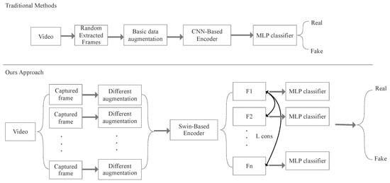
Figure 1.
Illustration of Swin-Fake framework compared with traditional deepfake video detector framework.
There are three main improvements in our method compared with traditional deepfake detectors: (1) We utilize five data augmentation methods, including base transformation, Random Erasing [12], Random Augmentation, Random Crop and DFDC Selim [13], which are randomly applied, and they will largely avoid over-fitting at the input stage. (2) Swin Transformer is chosen as the encoder, which will combine the correlations between different divided image patches. (3) The final total loss is determined by two components, which are consistency loss and cross-entropy loss, and the decision is guaranteed by consistency learning.
2. Related Work
2.1. Deepfake Detection
Deepfake detection is always defined as a binary classification or a multi-class classification work because it essentially requires the model to distinguish the media as real or fake. The most popular framework is to utilize vanilla Xception [14] or ResNet [15] as backbones to encode and then combine contrastive learning or explore representations’ consistency. Capsule Network [4] is an effective lightweight network which can solve “Inverse Graphic” problems and proposes a dynamic routing algorithm to regroup the extracted features. CORE [16] is a consistency learning method based on Xception Network which improves the number of data augmentations to prove the model’s consistency. Youtu-Lab [17] proposed a dual-contrastive learning architecture to distinguish the authenticity of faces using different data augmentations as well. Ensemble learning deepfake detectors could also significantly improve classification performance and have been widely applied in recent research; for example, Zhang [18] proposed a heterogeneous feature ensemble learning method to first extract gray gradient features, spectrum features and texture features from images, and then integrate them into an ensemble feature vector through a flattening process. Using DeepfakeStack, the authors of [19] chose to combine several state-of-the-art deepfake classification models to create an improved composite classifier which could reach 99.65% accuracy in some deepfake datasets. However, our proposed method, Swin-Fake, aims to explore the ability of Swin Transformer to extract forged features, such as PRNU noise and boundary mismatch, and then extract different frames of one video to prove the model’s consistency in the classification process using different data augmentations.
2.2. Swin Transformer
Swin Transformer [11] is a hierarchical Vision Transformer that improves multi-head attention blocks (MSAs) to window multi-head attention (W-MSAs) and shifted window multi-head attention blocks (SW-MSAs). It layers different sizes of features by setting up different sizes of windows, which is different from the traditional Vision Transformer [7], and could save more on computing costs than the traditional Vision Transformer. Normally the input image has a size of and the output feature size is . This framework contains one patch portion layer, one linear embedding layer and twelve Swin Transformer blocks to extract features, and the features are correlated with different patch embeddings. This network structure can more effectively simulate the sense of consistency and inconsistency of different patches when human eyes are observing and scanning different deepfake facial areas. Moreover, we investigated existing papers related to Transformer-based deepfake detectors, and surprisingly found there are not many papers focused on spatial consistency learning with a Transformer backbone. Most of them put more effort into designing temporal feature extraction blocks to obtain more temporal consistency information. Recently, Ilyas et al. [20] proposed an AVNet to detect audio–visual media using Swin Transformer, and Khalid [21] proposed utilizing Swin Y-Net for deepfake detection.
2.3. Data Augmentation
In the computer vision field, it is important to apply data augmentation, which is the first stage in preventing overfitting and an effective method to increase the amount of data. In this paper, we only utilize five image manipulation methods to change pixel values and positions. Base transformation is employed to combine pixel normalization and resizing. Random Erasing [12] is a cutout data transformation that randomly selects a rectangle block of the facial area and changes its color to totally black. Random Crop is used to crop the facial area in a random ratio and then resize it to a specific height and width. DFDC Selim is a complex data augmentation containing Gaussian noise, Gaussian blur, random shift and scale, and has already been proven to be the most useful data augmentation in deepfake classification work [16]. Random Augmentation randomly selects either Random Erasing, Random Horizontal Flip or Random Resize Crop. Compared with the design of traditional deepfake detectors, we have dramatically improved the diversity and randomness of input data, and it can be used for the subsequent verification of the similarity between different video frames of one video clip.
3. Proposed Methods
In this work, we outline the deepfake image detector pipeline and divide it into four parts: data pre-processing (including facial detection, crop and data augmentations), feature extraction, consistency calculation and prediction through classifiers. As shown in Figure 2, we first equally capture the frames of one detected video and randomly select and apply data augmentations to create different data views. After extracting the features through Swin Transformer, we separately calculate the cosine distances between representations in combinations and subtract the mean cosine distance as a consistency loss (See Algorithm 1). To prevent the unbalanced classes problem, we combine other databases’ real videos into our training set, which is very important for further evaluation; in addition, we also choose to up-sample the real video frames; for example, if every fake video is equally divided into eight frames, the real video frame is equally divided into 16 or 32 correspondingly. This could largely prevent the trained model’s predicted output from remaining in the same class.
| Algorithm 1 The workflow of Swin-Fake |
|
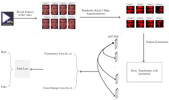
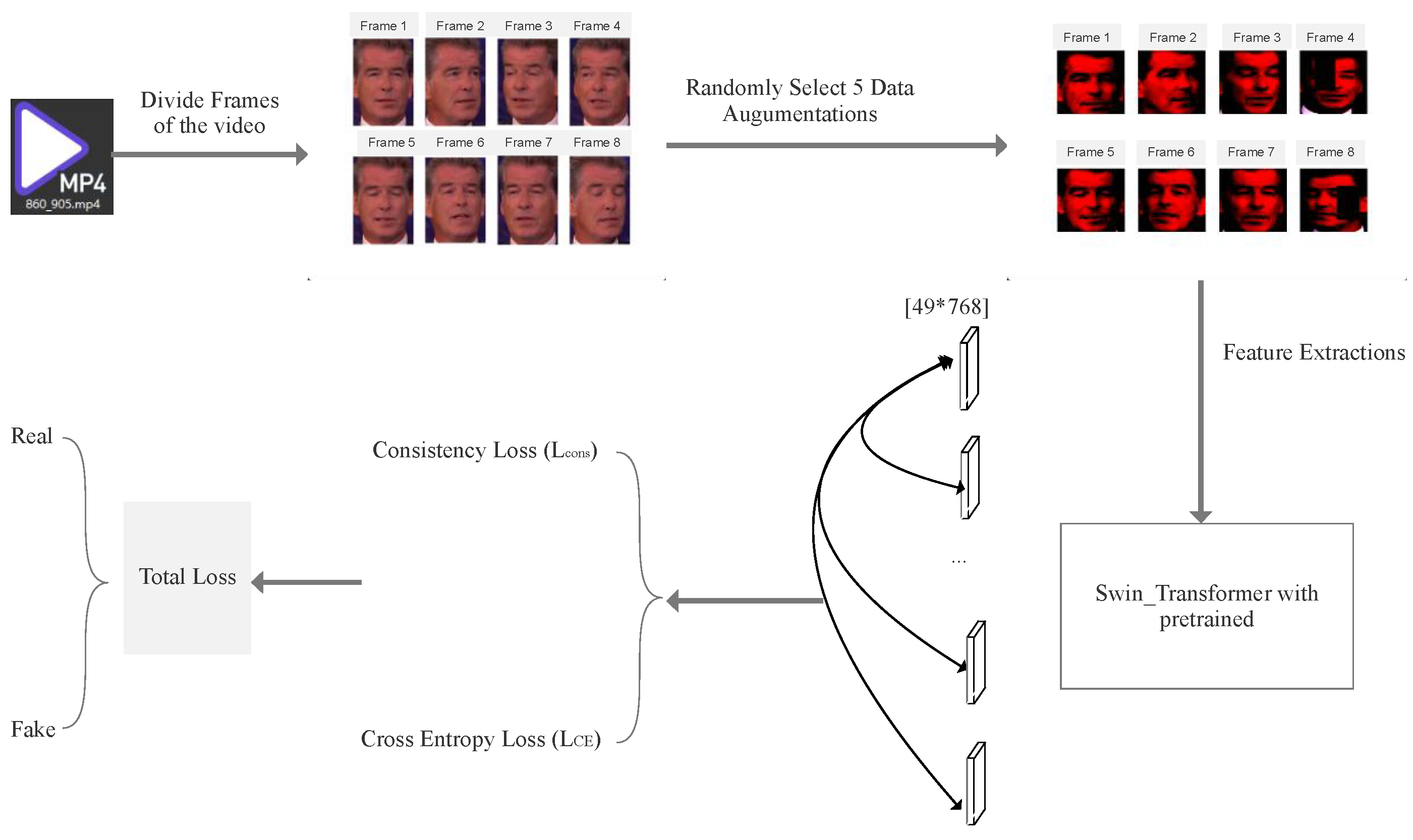
Figure 2.
Explanation of Swin-Fake architecture. We firstly divide M frames of one video and apply different data augmentations for each frame. Then, they are sent to a shared Swin Transformer encoder. After obtaining M representations, they will be sent to separately calculate classification loss and consistency loss.
3.1. Pre-Processing Work
Firstly, we give an input batch of B videos and equally divide each video into M video frames based on calculating each video’s total frame number. The pre-processing stage also embeds a facial detector, “SCRFD” [22] to locate facial areas, align the faces and crop them to create specific datasets. Specifically, this facial detector is based on Insightface and utilizes specific Sample Redistribution (SR) and Computation Redistribution (CR) methods for facial detection. “scrfd 10g kps.onnx” is one of the model weight files utilizing this face detection method [22], and kps represents the 5 facial key points detected in this model. To preserve some background information, we expand the width and height of the cropped images by 10%. Then, the total frames are neatly arranged in order, serving as the inputs for the Swin Transformer, and all resized to . Since we apply and randomly selected five data augmentations in a transformation set T on frames, the input vector sets I have a size of [B, M, 3, 224, 224] which means every group contains M [3, 224, 224] views. Finally, the input view set is written as:
where represents each frame view, B represents a batch of video, represents the B-th group of data views and M represents how many frames are equally divided.
Once the input data views are obtained, five data augmentation methods will be randomly applied on these data views. These augmented tensors are the final input of the Swin-Fake model’s inputs, as shown in Figure 3.
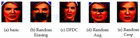
Figure 3.
Examples of random augmented data. For Random Erasing, we set the Random Erasing that will be performed to 0.8, the scale is from 0.02 to 0.2 and the erased area ratio is from 0.5 to 2.0. For Random Crop, we set the Random Crop scale from 0.77 to 1 and Random Crop ratio from 0.9 to 1.1.
3.2. Encoder Network
We adopt Swin Transformer [11] as our feature extractor f because of its unique hierarchical structure. It contains multiple stacking Transformer blocks, among which the lower-level blocks can capture some color and edge information and the higher-level blocks can be utilized to analyze the semantic information. After applying the shifted window partitioning approach and linear embedding, we can change the dimension of the input feature and obtain the query (Q), key (K) and value (V) vectors separately. The queries (Q) and keys (K) have the same dimension of d. By computing the dot products of the query (Q) with all keys (K) and dividing each by , the first step of the attention correlation is finished. Then, we add the bias and apply a softmax function to squeeze the output within the range of 0 to 1 and obtain a value score. This attention calculation method aims to compute the weighted sum of values, which is the same as “Scaled Dot-product Attention”. The calculation of self-attention is written as
where is the scaling factor of Q, K and B is the bias of Q, K, V.
When the input set I goes through the encoder and is mapped into representations, the representation is a two d-dimensional vector with a size of [49, 768]. Meanwhile, each M representation is set as one group and fed into the computation of consistency loss. After applying a linear layer on the last basic Swin block, we send the representations to compute Cross Entropy loss for classification. Thus, each batch of frames requires going through multiple data-augmented operations, and then, we can obtain the extracted low-dimensional features (See Figure 4). Finally, there will be two output vectors calculated, one for consistency loss calculation and another operated by the linear layer for classification loss. A detailed explanation of these two loss function calculations can be seen in Section 3.3.

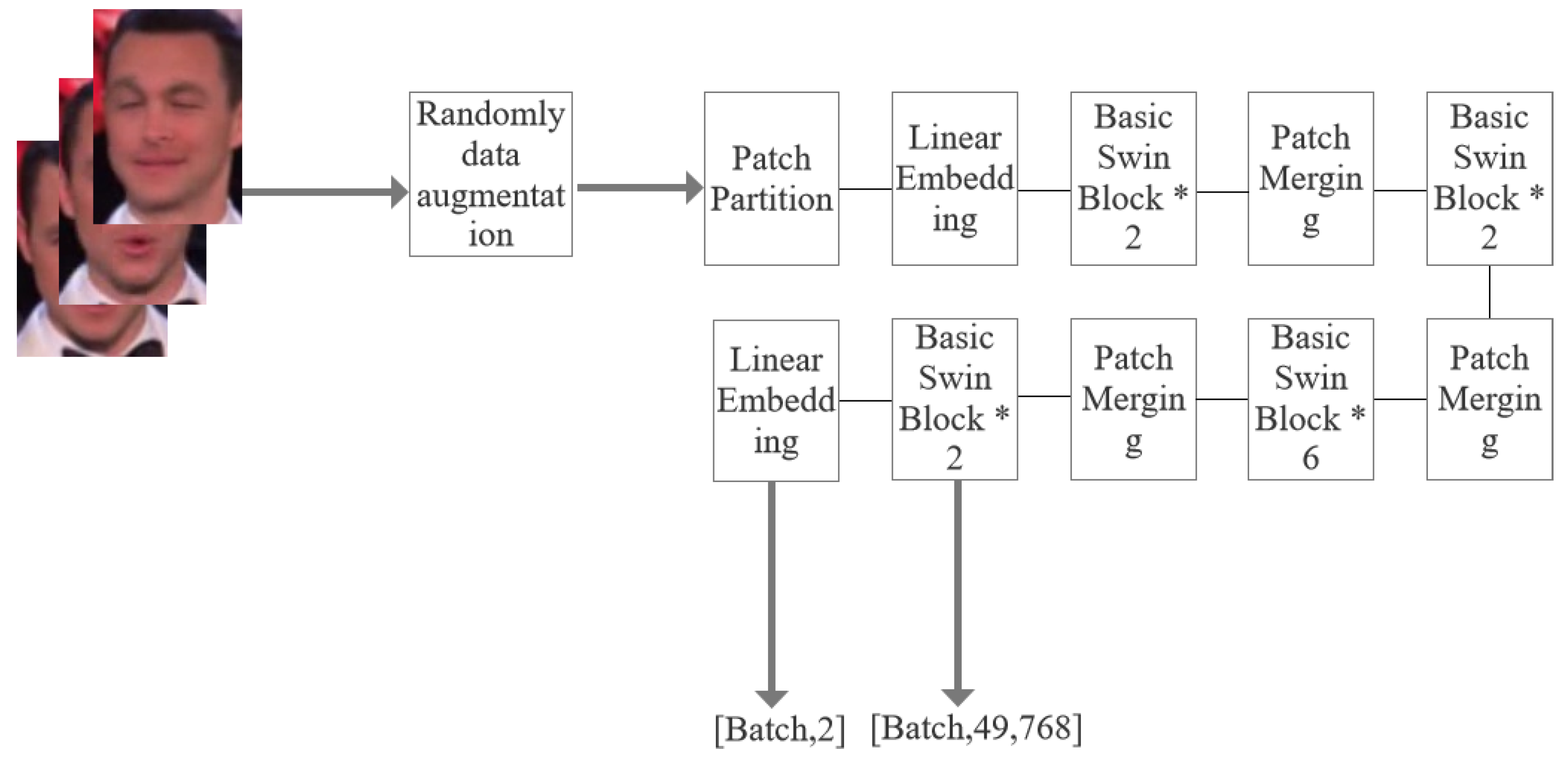
Figure 4.
The architecture of the Swin Transformer backbone. * represents how many Basic Swin Blocks are applied in the backbone. There are two output vectors for each input data view set in our model, which are the extracted low-dimensional features with a size of and the predicted probability .
3.3. Loss Functions
The loss function of this model is designed with two components: classification loss and consistency loss. Consistency loss is applied on each group of M extracted representations and we subtract their distances. In addition, the reason we adopt the cosine distance to complete the consistency loss design is that we do not force each pair of representations to be exactly the same but to be more and more similar. The cosine distance calculation of each pair of representations can be written as
where and represent the i-th and t-th frames of data views, and and represent the normalized representations extracted by a shared encoder.
Since we have obtained augmented video clips with the amount of B groups as the input of our model, we also need to calculate the similarity between these features of the captured video clips. The aim of this is to solve some incorrectly distinguished results of hard samples by shortening their cosine distances, and we regard this as consistency loss. As for another factor that influences the total loss, consistency loss is designed to calculate the mean cosine distances of B batch videos. Specifically, the extracted M representations of one video can generate pairs of similarities through the above equation. The single consistency of one video can be expressed as the mean of pair similarity, and the total consistency loss of B batch videos requires us to calculate the average value of all the calculated single consistencies. Therefore, the consistency loss can be written as
where B represents the batch size of the video.
The main purpose of setting up consistency loss is to prove that no matter how realistic one particular deepfake video frame is, the model is able to shorten its spatial distance with other forgery frames. On the other hand, consistency loss validates the classification consistency of different frames of one video. Since the classification work is inseparable from supervised labels, we apply standard cross-entropy loss as classification loss, and we formulate it as follows:
where y is the ground truth label, p is the predicted probability, and represents the total number of video frames.
Because our model is a consistency learning model, we utilize two loss functions (consistency loss and cross-entropy loss) in the linear combination to form our total loss. However, we set the hyper-parameter as the weight balance to observe what proportion of these two loss functions can reach the minimum total loss and reach the highest accuracy. In Section 4.4, we conduct one ablation test to observe what value of this hyper-parameter can predict the most samples by traversing the weight parameter by adding 0.1 in every experiment, because we hope to find out the best fitting weight to balance these two loss functions, and we do not hope the total loss is largely biased toward one of the loss functions’ results.
where is the hyper-parameter to balance cross entropy loss and consistency loss, and it ranges from 0 to 1.
4. Experiments
4.1. Datasets
To evaluate our method, we selected four common datasets in this field: FaceForensics++ [23], DFDC [24], Celeb-DF [25] and FaceShifter [26]. In particular, the first two datasets were used for the training phase, and Celeb-DF V2 and FaceShifter were used for cross-dataset experiments to prove our model’s generalization ability. FaceForensics++ is a pioneering large-scale dataset in facial manipulation which contains 1000 real videos and 4000 fake videos generated by Face2Face, FaceSwap, Neural Textures and Deepfakes. DFDC is the largest datasets of these four datasets, containing 119,197 videos filmed by real actors. Compared with the previous two datasets, Celeb-DF is derived from 590 original YouTube videos and 5639 manipulated videos with advanced color blending, which is hard to distinguish by human eyes. FaceShifter is one sub-class of FaceForensics++ datasets, and it contains 1000 fake videos with different shooting scenarios. Considering the imbalanced training data of FaceForensics++, we randomly combined 2000 real videos from the DFDC database with real FF++ videos to solve this problem. As for the DFDC training, we chose to down-sample some fake video frames to solve the data imbalance.
4.2. Implementation Details
For data pre-processing, we extracted M frames of each video by setting a confidence threshold of 0.5 and an NMS threshold of 0.5 for “scrfd 10g kps.onnx”. In addition, the detected cropped faces with bounding boxes were enlarged by 1.2 both in width and height to ensure there existed some background information on the model’s inputs. As for the data augmentation settings, we set an 80% probability of erasing the facial area, the range of the proportion of the erased area against the input image was set from 0.02 to 0.2, and the range of the aspect ratio of the erased area was set from 0.5 to 2.0 in the Random Erasing operation. In the Random Crop augmentation, we set the scale’s lower and higher bounds to 0.77 and 1, which means the random area of cropping before resizing was from 0.77 to 1 correspondingly. During the experiment, some selected frames (See Figure 5) with no human faces were copied from the last detected index frame instead of being directly sent to the input data view set.
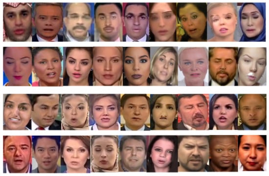
Figure 5.
Some deepfake samples processed by “scrfd 10g kps.onnx”, which is the original input for our model training.
For model training, we set the video mini-batch size to 4 with an image size of , and then utilized an AdamW optimizer [27] with weight decay set to 0.05 and the learning rate set to 0.0001. To effectively train this model, we stopped training early if there was no increase in validating accuracy in the first 5 epochs, and the total epoch was set to 30. In addition, all the dropout rates were set to 0.2 avoid over-fitting in our experiment. All our models used swin-tiny-patch4-window7-224.pth and were pre-trained on ImageNet-1K as the backbone, and the output features were extracted by the linear layer with a size of and the vectors with a size of . We initially adopted a balanced weight of 0.5 because we regarded consistency loss as having the same importance as classification loss at the beginning.
4.3. In-Dataset Study
In this section, we evaluate our proposed model’s validating performance in the same sources as the training datasets. For the in-dataset experiments, we assessed DFDC and FaceForensics++, which are two relatively large datasets, because we found that Swin Transformer always requires a large amount of training data to reach a good validation level during training experiments; otherwise, it will present a relatively low starting validating accuracy in some small-scale training datasets. And the initial hyper-parameter was set to 0.5 as default. We compared our consistency learning method with three baselines: Capsule Network, STIL [28] and ISTVT [10]. As shown in Table 1, Capsule Network presents the lowest accuracy and ISTVT performs better than STIL. Our approach performs much better than Capsule Network, and the in-dataset accuracy is a little bit higher than that of STIL and ISTVT.

Table 1.
Deepfake detection accuracy. The best in-datasets accuracy results are bolded. Except for Capsule Network, which is reproduced, the other methods’ results are from [10,28].
4.4. Ablation Test Results
To test the significance of the consistency branch of our model, we also conducted an ablation experiment (see Table 2) on Swin Transformer deepfake image classification with our approach (with consistency learning supervised). We found that consistency learning can effectively increase the accuracy, which is because our approach uses consistency loss to shorten the distances (increases the similarity) between different frames of the video so that if one frame is distinguished by the classification branch as fake with a really high confidence score, there is a high probability that other hard sample frames will be regarded as fake as well.
Table 2.
Ablation experiment accuracy comparison. We utilized Swin Transformer to conduct a deepfake image binary test and compare its accuracy with that of our approach.
In addition, the balance weight is another variable that decides the final total loss; thus, we conducted an ablation experiment to determine how much weight is required for the consistency loss to show the best performance in this discriminative model by setting this hyper-parameter to 0.4, 0.5, 0.6, 0.7 and 0.8. In this ablation test, we still utilized FaceForensics++ as the dataset to explore what balance weight could reach the highest predicted accuracy. In addition, we combined all the fake categories into one class to test binary performance instead of testing multiple classifications. Because we did not set this weight balance as a learnable parameter in our model, we chose to traverse the weight balance by adding 0.1 per experiment. Once we obtained the highest accuracy, we regarded this model as the state-of-the-art model, and we utilized this model’s trained parameters to conduct cross-dataset experiments. As shown in Table 3, we find that the weight balance setting of 0.7 shows the best performance, and was trained on the FaceForensics++ binary test.
Table 3.
Ablation experiment accuracy on different weight balances. This is to test which weight balance of our loss function will achieve the best result.
4.5. Cross-Dataset Study
Due to the multiple forgery methods, it is important to evaluate the model’s cross-dataset performance. To test the generalization ability of our model, we trained our model on FaceForensics++ and tested it on Celeb-DF, FaceShifter and DFDC. Considering that most deepfake datasets’ sample sizes for the real class and fake class are unbalanced, we also chose to utilize the Area Under the Curve (AUC) to evaluate the robustness of our model, as shown in Table 4.
Table 4.
The AUC of the cross-dataset experiment. We trained our model on FF++ and tested the unseen data. The best cross-dataset AUC results are bolded. The other methods’ results are from [10,28,29,30,31].
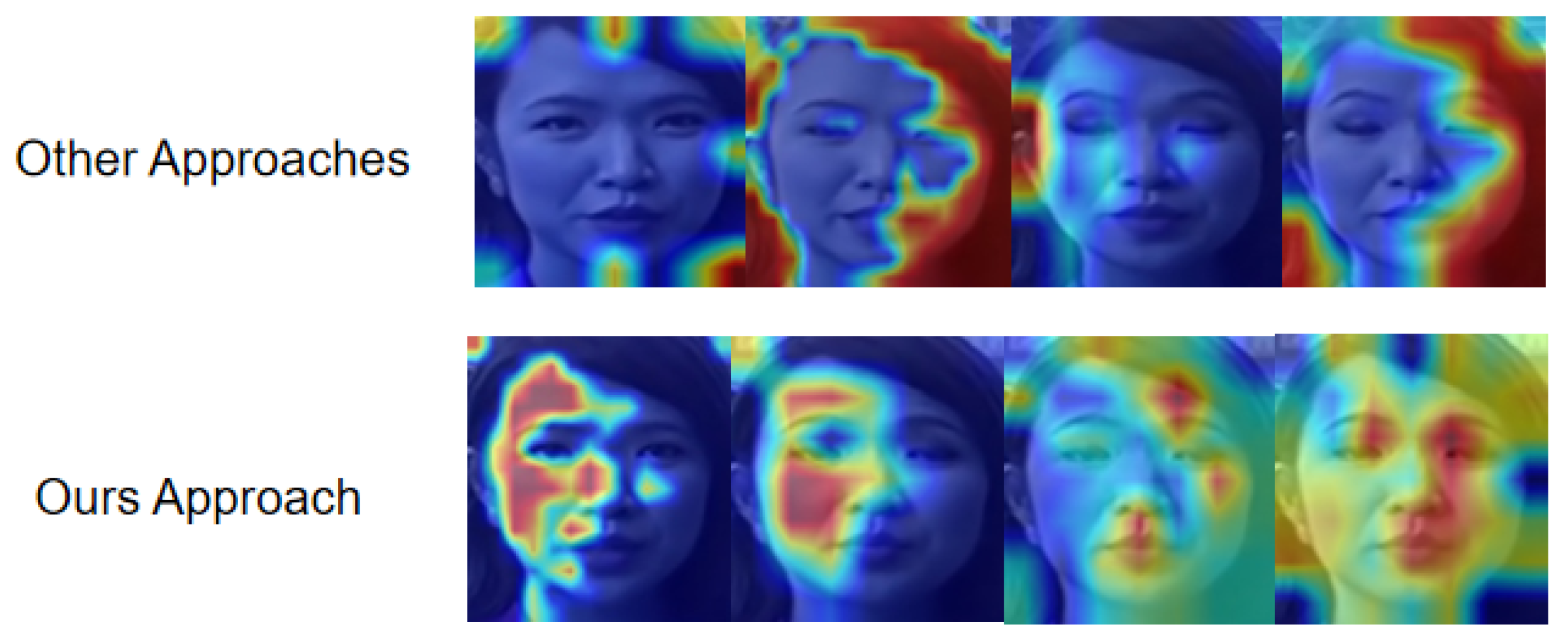
We found that our approach could only have the best results on Celeb-DF. This is because Celeb-DF contains advanced post-processing work such as color blending and it is really hard to find out when boundary mismatch happens in generated media. To prove this point of view, we chose to create heatmaps of our model and other CNN-based detection models to explain the model’s visualization of focus regions of deepfake media. By observing the heatmap of our model, we found that our model focuses more on generated human facial contents such as lips and eyes instead of boundary texture information (see Figure 6). By checking some example videos of FaceShifter, we found that forgery clues always happen in the facial boundary area, which is the facial region that our model pays less attention to, but Celeb-DF’s forgery clues occur on the facial features, such as unnaturally manipulated human eyes and lips. In addition, we compared the data in Celeb-DF with the data of DFDC, and we found that DFDC contains more data with different shooting scenarios, such as dark indoor backgrounds and faces with extreme poses. This makes it really hard for our model to achieve consistency and obtain useful information to distinguish real or fake media because we utilized the model trained by FaceForensics++, and it included more human faces with normal poses and bright shooting scenarios, which is similar to the Celeb-DF data distribution.
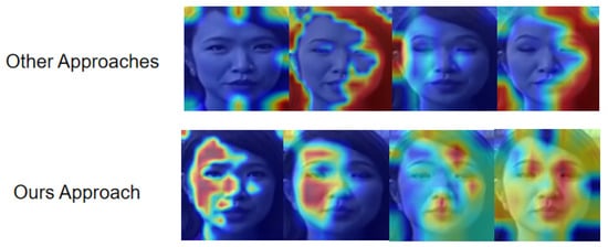
Figure 6.
Comparison heatmap between other deepfake detector methods and our approach. From this figure, it is obvious that most deepfake detectors focus on boundary information of generated fake media.
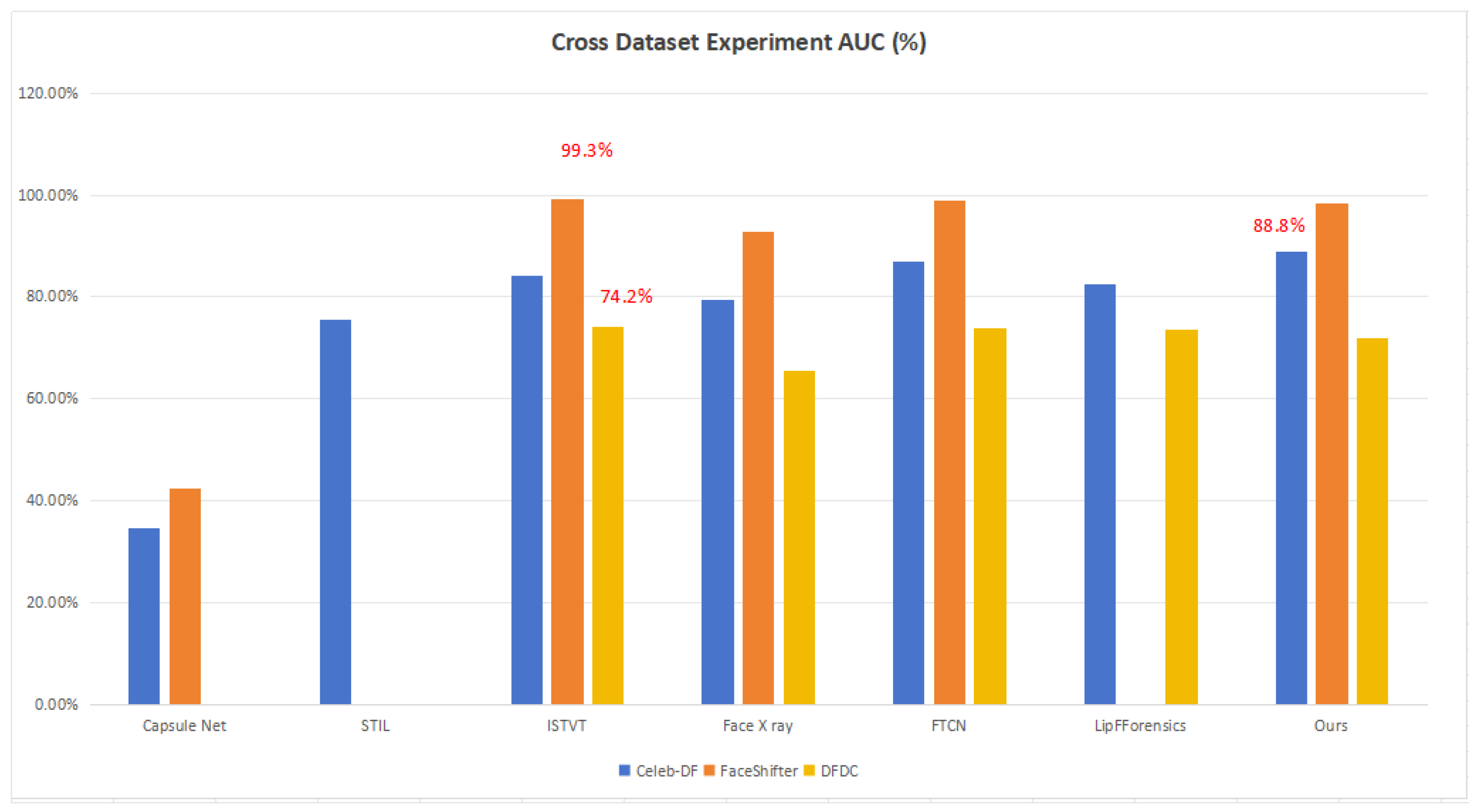
In addition, we also compared the Transformer-based method ISTVT as a benchmark model, and it achieved slightly better AUC results on FaceShifter and DFDC (see Figure 7). This is because the authors who used ISTVT applied a self-subtraction mechanism and temporal self-attention in their work, which is what our approach lacks. The self-subtraction mechanism can focus more on inter-frame distortion, which is another significant technique for deepfake detection. It requires the application of an input token before the projection to query and key vectors. It generates feature residuals to replace the original features. However, our model still achieves competitive results compared with other previous state-of-the-art models such as STIL and Face X-ray.
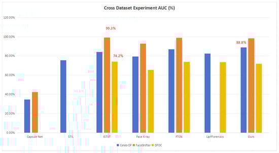
Figure 7.
Cross-dataset AUC results based on Capsule Net, STIL, ISTVT, Face X-ray, FTCN, LipForensics and our approach. The best performance on each dataset is labeled in the figure.
5. Conclusions and Future Work
In this paper, we propose Swin-Fake, which, for the first time, combines Swin Transformer with consistency loss, as a consistency learning method for deepfake detection. We employ Swin Transformer as the feature extractor and utilize the average Cosine distance as a measure of consistency loss, which improved generalization ability in some deepfake databases. We proved that a Transformer-based classifier could reach a higher level in the deepfake detection field compared with other previous CNN-based methods. During the training and validation phases, we concluded that Swin Transformer had better deepfake distinguishing ability, while large-scale databases such as FF++ and DFDC do not exhibit promising performance on some small datasets such as Celeb DF. In addition, calculating the consistency between the frames’ features could significantly decrease the loss and enhance the evaluation metrics; thus, we believe that applying the consistency learning method with Transformer for deepfake detection could be a new trend in fake media detection.
Deepfake video detection cannot be completed without temporal information because frame jittering always happens in the adjacent frames. In recent research, temporal attention is always combined with spatial attention for video detection. As another technique in the video detection field, temporal attention can be seen as a dynamic temporal selection mechanism that determines when to pay attention to a certain feature of a video, and is often applied in video processing. It is also an effective method to increase the evaluation metrics in this field if we can combine temporal consistency information together with extracted spatial information, and the most common method is to design a specific modules to explore temporal consistency or inconsistency by applying horizontal and vertical convolutional layers. Thus, in future work, we will further investigate temporal self-attention of the Swin Transformer-based backbone. Even though our current work is focused on video-based detectors, we still focus on spatial feature extraction, and feature consistency is applied for intra-class comparison. Combining temporal consistency with spatial consistency would probably involve more information, which would benefit the classification of videos. As for the weight balance , we added 0.1 in each experiment to test the efficiency of the consistency block and obtain the value with the highest accuracy. To obtain a more accurate value of this hyper-parameter, we will set the weight balance as a learnable parameter in future investigations. Additionally, we will further investigate other visualization methods for Swin Transformer-based deepfake detectors to interpret what spatial features are captured and contribute to the deepfake classifier.
Author Contributions
Conceptualization, L.Y.G. and X.J.L.; methodology, L.Y.G. and X.J.L.; software, L.Y.G.; validation, L.Y.G.; formal analysis, L.Y.G.; investigation, L.Y.G.; resources, L.Y.G. and X.J.L.; data curation, L.Y.G. and X.J.L.; writing—original draft preparation, L.Y.G., X.J.L. and P.H.J.C.; writing—review and editing, L.Y.G., X.J.L. and P.H.J.C.; visualization, L.Y.G. and X.J.L.; supervision, X.J.L. and P.H.J.C.; project administration, X.J.L. and P.H.J.C. All authors have read and agreed to the published version of the manuscript.
Funding
This research received no external funding.
Data Availability Statement
The relative datasets are downloaded from [24], DFDC reproduced codes are from [13].
Conflicts of Interest
The authors declare no conflicts of interest.
References
- Goodfellow, I.; Pouget-Abadie, J.; Mirza, M.; Xu, B.; Wared-Farley, D.; Ozair, S.; Courville, A.; Bengio, Y. Generative Adversarial Network. Commun. Acm 2018, 63, 139–144. [Google Scholar] [CrossRef]
- Karras, T.; Laine, S.; Aila, T. A style-based generator architecture for generative adversarial networks. In Proceedings of the IEEE/CVF Conference on Computer Vision and Pattern Recognition, Long Beach, CA, USA, 15–20 June 2019. [Google Scholar]
- Ho, J.; Jain, A.; Abbeel, P. Denoising Diffusion Probabilistic Models. In Proceedings of the 34th International Conference on Neural Information Processing System, Red Hook, NY, USA, 6–12 December 2020; pp. 6840–6851. [Google Scholar]
- Nguyen, H.H.; Yamagishi, J.; Echizen, I. Use of a Capsule Network to Detect Fake Images and Videos. In Proceedings of the Computer Vision and Pattern Recognition, Long Beach, CA, USA, 16–20 June 2019. [Google Scholar]
- Das, S.; Seferbekov, S.; Datta, A.; Islam, M.S.; Amin, M.R. Towards solving the deepfake problem: An analysis on improving deepfake detection using dynamic face augmentation. In Proceedings of the IEEE/CVF International Conference on Computer Vision, Montreal, BC, Canada, 11–17 October 2021. [Google Scholar]
- Zhao, T.; Xu, X.; Xu, M.; Ding, H.; Xiong, Y.; Xia, W. Learning Self-Consistency for Deepfake Detection. In Proceedings of the IEEE/CVF Conference on Computer Vision and Pattern Recognition, Nashville, TN, USA, 20–25 June 2021. [Google Scholar]
- Dosovitskiy, A.; Beyer, L.; Kolesnikov, A.; Weissenborn, D.; Zhai, X.; Unterthiner, T.; Dehghani, M.; Minderer, M.; Heigold, G.; Gelly, S.; et al. An Image is Worth 16 × 16 Words: Transformers for Image Recognition at Scale. In Proceedings of the International Conference on Learning Representations, Virtual, 26 April–1 May 2020. [Google Scholar]
- Khan, S.A.; Dai, H. Video Transformer for Deepfake Detection with Incremental Learning. In Proceedings of the 29th ACM International Conference on Multimedia, Virtual Event, 20–24 October 2021; pp. 1821–1828. [Google Scholar]
- Khormali, A.; Yuan, J. DFDT: An End-to-End DeepFake Detection Framework Using Vision Transformer. Appl. Sci. 2022, 12, 2953. [Google Scholar] [CrossRef]
- Zhao, C.; Wang, C.; Hu, G.; Chen, H.; Liu, C.; Tang, J. ISTVT: Interpretable Spatial-Temporal Video Transformer for Deepfake Detection. IEEE Trans. Inf. Forensics Secur. 2023, 18, 1335–1348. [Google Scholar] [CrossRef]
- Liu, Z.; Lin, Y.; Cao, Y.; Hu, H.; Wei, Y.; Zhang, Z.; Lin, S.; Guo, B. Swin Transformer: Hierarchical Vision Transformer using Shifted Windows. In Proceedings of the IEEE/CVF International Conference on Computer Vision, Montreal, BC, Canada, 11–17 October 2021. [Google Scholar]
- Zhong, Z.; Zheng, L.; Kang, G.; Li, S.; Yang, Y. Random Erasing Data Augmentation. In Proceedings of the AAAI Conference on Artificial Intelligence, New York, NY, USA, 7–12 February 2020. [Google Scholar]
- DFDC Selim. Available online: https://github.com/selimsef/dfdc_deepfake_challenge (accessed on 15 May 2024).
- Chollet, F. Xception: Deep learning with depthwise separable convolutions. In Proceedings of the Computer Vision and Pattern Recognition, Honolulu, HI, USA, 21–26 July 2017. [Google Scholar]
- He, K.; Zhang, X.; Ren, S.; Sun, J. Deep Residual Learning for Image Recognition. In Proceedings of the 2016 IEEE Conference on Computer Vision and Pattern Recognition, Las Vegas, NV, USA, 27–30 June 2016. [Google Scholar]
- Ni, Y.; Meng, D.; Yu, C.; Quan, C.B.; Ren, D.; Zhao, Y. CORE: Consistent Representation Learning for Face Forgery Detection. In Proceedings of the IEEE/CVF Conference on Computer Vision and Pattern Recognition, New Orleans, LA, USA, 18–24 June 2022. [Google Scholar]
- Sun, K.; Yao, T.; Chen, S.; Ding, S.; Li, J.; Ji, R. Dual Contrastive Learning for General Face Forgery Detection. AAAI Conf. Artif. Intell. 2022, 36, 2316–2324. [Google Scholar] [CrossRef]
- Zhang, J.; Cheng, K.; Sovernigo, G.; Lin, X. A Heterogeneous Feature Ensemble Learning based Deepfake Detection Method. In Proceedings of the ICC 2022—IEEE International Conference on Communications, Seoul, Republic of Korea, 16–20 May 2022; pp. 2084–2089. [Google Scholar]
- Rana, M.S.; Sung, A.H. DeepfakeStack: A Deep Ensemble-based Learning Technique for Deepfake Detection. In Proceedings of the 2020 7th IEEE International Conference on Cyber Security and Cloud Computing (CSCloud)/2020 6th IEEE International Conference on Edge Computing and Scalable Cloud (EdgeCom), New York, NY, USA, 1–3 August 2020; pp. 70–75. [Google Scholar]
- Ilyas, H.; Javed, A.; Malik, K.M. AVFakeNet: A unified end-to-end Dense Swin Transformer deep learning model for audio–visual deepfakes detection. Appl. Soft Comput. 2023, 136, 110124. [Google Scholar] [CrossRef]
- Khalid, F.; Akbar, M.H.; Gul, S. SWYNT: Swin Y-Net Transformers for Deepfake Detection. In Proceedings of the 2023 International Conference on Robotics and Automation in Industry (ICRAI), Peshawar, Pakistan, 3–5 March 2023; pp. 1–6. [Google Scholar]
- Guo, J.; Deng, J.; Lattas, A.; Zafeiriou, S. Sample and Computation Redistribution for Efficient Face Detection. In Proceedings of the International Conference on Learning Representation, Virtual Event, 3–7 May 2021. [Google Scholar]
- Zhou, T.F.; Wang, W.G.; Liang, Z.Y.; Shen, J.B. Face Forensics in the Wild. In Proceedings of the Computer Vision and Pattern Recognition (CVPR), Virtual, 19–25 June 2021. [Google Scholar]
- Kaggle. Available online: https://www.kaggle.com/c/deepfake-detection-challenge/overview (accessed on 12 December 2023).
- Li, Y.Z.; Yang, X.; Sun, P.; Qi, H.G.; Lyu, S. Celeb-DF: A Large-scale Challenging Dataset for DeepFake Forensics. In Proceedings of the Computer Vision and Pattern Recognition, Seattle, WA, USA, 14–19 June 2020. [Google Scholar]
- Li, L.; Bao, J.; Yang, H.; Chen, D.; Wen, F. FaceShifter: Towards High Fidelity And Occlusion Aware Face Swapping. In Proceedings of the IEEE/CVF Conference on Computer Vision and Pattern Recognition, Seattle, WA, USA, 13–19 June 2020. [Google Scholar]
- Loshchilov, I.; Hutter, F. Decoupled weight decay Regularization. In Proceedings of the International Conference on Learning Representations, New Orleans, LA, USA, 6–9 May 2019. [Google Scholar]
- Gu, Z.; Chen, Y.; Yao, T.; Ding, S.; Li, J.; Huang, F.; Ma, L. Spatiotemporal Inconsistency Learning for Deepfake Video Detection. In Proceedings of the IEEE/CVF Conference on Computer Vision and Pattern Recognition, Virtual, 19–25 June 2021. [Google Scholar]
- Li, L.; Bao, J.; Zhang, T.; Yang, H.; Chen, D.; Wen, F.; Guo, B. Face X-ray for More General Face Forgery Detection. In Proceedings of the IEEE/CVF Conference on Computer Vision and Pattern Recognition, Seattle, WA, USA, 13–19 June 2020. [Google Scholar]
- Zheng, Y.; Bao, J.; Chen, D.; Zeng, M.; Wen, F. Exploring temporal coherence for more general video face forgery detection. In Proceedings of the IEEE/CVF International Conference on Computer Vision, Montreal, QC, Canada, 10–17 October 2021; pp. 15044–15054. [Google Scholar]
- Haliassos, A.; Vougioukas, K.; Petridis, S.; Pantic, M. Lips don’t lie: A generalisable and robust approach to face forgery detection. In Proceedings of the IEEE/CVF Conference on Computer Vision and Pattern Recognition, Virtual, 19–25 June 2021; pp. 5039–5049. [Google Scholar]


Disclaimer/Publisher’s Note: The statements, opinions and data contained in all publications are solely those of the individual author(s) and contributor(s) and not of MDPI and/or the editor(s). MDPI and/or the editor(s) disclaim responsibility for any injury to people or property resulting from any ideas, methods, instructions or products referred to in the content. |
© 2024 by the authors. Licensee MDPI, Basel, Switzerland. This article is an open access article distributed under the terms and conditions of the Creative Commons Attribution (CC BY) license (https://creativecommons.org/licenses/by/4.0/).