Abstract
Unmanned surface vehicles (USVs) in nearshore areas are prone to environmental occlusion and electromagnetic interference, which can lead to the failure of traditional satellite-positioning methods. This paper utilizes a visual simultaneous localization and mapping (vSLAM) method to achieve USV positioning in nearshore environments. To address the issues of uneven feature distribution, erroneous depth information, and frequent viewpoint jitter in the visual data of USVs operating in nearshore environments, we propose a stereo vision SLAM system tailored for nearshore conditions: SP-SLAM (Segmentation Point-SLAM). This method is based on ORB-SLAM2 and incorporates a distance segmentation module, which filters feature points from different regions and adaptively adjusts the impact of outliers on iterative optimization, reducing the influence of erroneous depth information on motion scale estimation in open environments. Additionally, our method uses the Sum of Absolute Differences (SAD) for matching image blocks and quadric interpolation to obtain more accurate depth information, constructing a complete map. The experimental results on the USVInland dataset show that SP-SLAM solves the scaling constraint failure problem in nearshore environments and significantly improves the robustness of the stereo SLAM system in such environments.
1. Introduction
Unmanned Surface Vehicles (USVs) have been widely applied in tasks such as ocean mapping and reservoir inspection in recent years. Since the 1980s, USVs have also been used for military missions [1,2]. Modern USVs are extensively utilized in various water engineering projects [3]. For example, in Wang’s research project [4], a USV-UAV joint system was deployed to complete maritime search and rescue tasks using visual navigation and reinforcement learning techniques. In Artur’s project [5], a USV was used for depth detection in extremely shallow waters at a public beach in Gdynia, Poland. Oktawia [6] employed a USV to collect datasets for a 3D reconstruction project in coastal areas.
The aforementioned examples are all typical cases of USVs operating in nearshore environments. The key to autonomous operations in such settings is accurate self-localization and environmental perception, enabling the vessel to avoid collisions and navigate effectively. Traditional methods employ the Automatic Identification System (AIS) [7] and satellite-based positioning. However, nearshore environments present challenges such as environmental occlusion and electromagnetic interference, which affect the accuracy of satellite-positioning methods [8]. Consequently, researchers have proposed using measurement-based methods to perceive the surrounding environment and achieve self-localization. Ma et al. [9] utilized a method that fuses radar and satellite images to determine the position of USVs, which proved effective in open ocean areas beyond 100 m from the shoreline. However, in nearshore environments, the accuracy was limited by the resolution of satellite images. Han et al. [10] employed marine radar and a SLAM framework for navigation relative to the coastline in coastal areas, but the complexity of nearshore environments introduced significant radar data noise, resulting in unnecessary measurements and insufficient localization accuracy. Liu et al. [11] designed an adaptive algorithm based on unscented Kalman filtering to predict the trajectory of USVs and restore position information when satellite signals were unavailable, but the method was ineffective during manually controlled turns and sudden stops. The underwater helicopter for coastal monitoring developed by Broman et al. [12] used traditional GPS positioning methods, achieving an accuracy of approximately 5 m in coastal areas, and obtained relevant profile information.
For small- to medium-sized USVs operating in nearshore environments, it is crucial to balance equipment cost and localization accuracy. Therefore, we are dedicated to exploring low-cost yet high-accuracy localization methods for USVs in nearshore environments.
Cost-effective visual localization technologies have gradually matured in recent years. One of the most classic visual odometry (VO) systems was employed on NASA’s Mars rovers [13], using a VO system equipped with stereo cameras to detect and compensate for unexpected rover slippage. Visual Simultaneous Localization and Mapping (VSLAM) algorithms based on visual odometry have been successfully applied to mobile robots [14]. In 2005, Nister [15] developed SLAM technologies for ground vehicle navigation, achieving error rates generally less than . Trujillo and colleagues’ [16] collaborative VSLAM system, when applied to drones, validates the feasibility of using VSLAM for localization in special circumstances when GPS signals fail.
Nearshore environments primarily refer to areas near the shoreline, including onshore structures, coastal vegetation, and water bodies within 50 m of the shore. These environments are common in all kinds of water, as illustrated in Figure 1. Nearshore environments are significantly different from indoor environments. Nearshore environment images typically contain reflections and ripples, as shown in Figure 1a. This poses a challenge for feature extraction, as the strong light regions present in ripples often result in feature points being extracted. However, as ripples change in each frame, it becomes difficult to track continuous ripple features, and a large number of ripple features will affect the matching accuracy. Additionally, frequent viewpoint jitter occurs when USVs operate on the water surface, making feature tracking difficult. Moreover, the open nature of nearshore environments complicates the measurement of depth information.
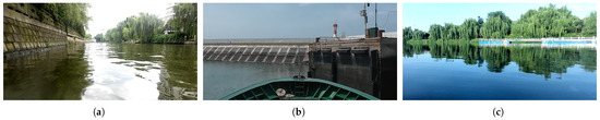
Figure 1.
Nearshore environments image, (a) is the river channel, (b) is the coastal area, and (c) is the lake.
To address the aforementioned issues, this paper proposes a stereo VSLAM algorithm suitable for nearshore environments. This method is based on ORB-SLAM2 [17] and incorporates relevant improvements tailored to the visual characteristics of nearshore environments. The specific improvements are as follows:
1. To address the issue of anomalous depth information of feature points in open environments, we design a distant segmentation method for images in nearshore environments. This method labels feature information from different regions and adaptively filters outliers during the optimization.
2. We improve the stereo depth estimation method by introducing the Sum of Absolute Differences (SAD) to match image blocks and perform quadric interpolation, thereby obtaining sub-pixel accuracy in depth information.
3. In order to tackle the issues caused by water surface reflections and ripples, we convert the uncertainty of each estimation from a Hessian matrix into a scalar and use a sliding window to monitor and correct errors.
2. Related Work
SLAM technology enables robots to construct maps in real time and accurately determine their position within unknown environments. Depending on the application domain, SLAM can be categorized into topological approaches, which provide high-level global navigation, and metric approaches, which are used for detailed local navigation and obstacle avoidance [18]. This paper primarily focuses on the latter, i.e., considering environmental geometric information, constructing environmentally meaningful maps, and achieving real-time localization. This localization method has already been employed in many autonomous driving technologies, such as Adaptive Cruise Control (ACC), Lane Keeping Assistance (LKA), and Automatic Emergency Braking (AEB) systems, which help drivers avoid collisions [19]. Metric methods can be further divided into direct methods and feature-based methods.
The direct method estimates camera motion by minimizing the photometric error between consecutive frames, where photometric error is defined as the difference in pixel intensity between images. This method is based on the assumption of brightness constancy in local regions of the image sequence. Representative algorithms of this method include DTAM [20], LSD-SLAM [21], and SVO [22]. Although this technique can directly process input images, it is extremely sensitive to changes in illumination, making it unsuitable for nearshore environments with significant lighting variations. In contrast, the feature-based method uses some representative content in the image to indirectly represent the image, typically in the form of point features. By continuously tracking these point features in sequential frames and minimizing the reprojection error, the camera’s pose can be recovered to achieve localization and mapping. Representative algorithms of this method include PTAM [23] and ORB-SLAM [24]. However, in low-texture scenes, where features are difficult to extract and there are insufficient parameters to construct the equation for minimizing the reprojection error, the accuracy of localization may fail completely.
In nearshore environments, significant lighting variations are prevalent. To address this issue, researchers have adopted many methods such as lighting adaptation and semantic segmentation. Li et al. [25] developed an improved ORB-SLAM algorithm suitable for low-light environments, which uses adaptive correction of environmental colors in the HVS space of the image to extract more features, thereby improving the algorithm’s accuracy under low-light conditions. The stereo visual SLAM algorithm based on dynamic feature filtering designed by Tian et al. [26] was once utilized by us to eliminate water surface ripple features, but unfortunately, it did not yield the desired results. The VSLAM system incorporating semantic segmentation designed by Ai et al. [27,28] did not perform effectively in the expansive dynamic environments of nearshore waters.
To address issues such as frequent viewpoint jitter and erroneous depth information, researchers have explored both traditional methods and emerging deep learning techniques. Wei [29] utilized guided points and dynamic programming to accelerate the matching process and employed adaptive filtering to effectively remove environmental noise. Kavitha et al. [30] used convolutional neural networks for the extraction and matching of binocular image features, and experiments demonstrated that this method achieved excellent performance in large-scale image matching and depth measurement. Lin et al. [31] deployed multiple visual sensors and set up circular constraints to guide device motion, generating disparity from multiple viewpoints and calculating the depth of environmental features. They constructed a prototype device for rotational depth measurement, which showed promising results in experiments.
There are relatively few cases of using visual SLAM for USV positioning in water surface scenarios. Zou et al. [32,33] employed the WSD algorithm to segment water surface scenes into water and non-water regions, simplifying the computation by fixing the camera in a specific position. Their experiments demonstrated the robustness of this method. Ystein et al. [34] designed a positioning system that combines visual and acoustic data, achieving precise localization with an error margin of less than in port and channel areas. David et al. [35] implemented a traditional monocular visual odometry system in urban inland waterways. Due to the abundant structural features provided by the buildings along the riverbanks, this approach yielded excellent results.
3. SP-SLAM Method
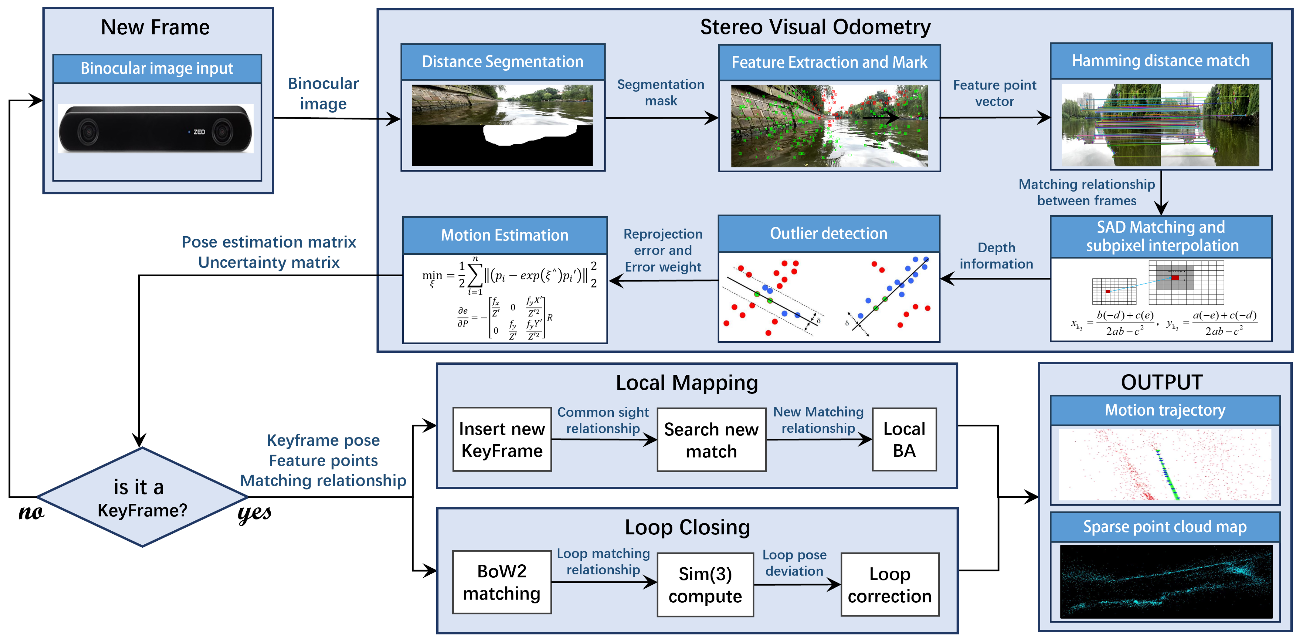
The overall structure of the proposed SP-SLAM system is illustrated in the accompanying Figure 2. This structure is derived from the well-established ORB-SLAM2 and comprises three distinct threads: visual odometry, local mapping, and loop closure. In the visual odometry thread, we incorporate a distance segmentation module to label feature points in different regions and adaptively filter outliers during optimization, while also refining the depth estimation algorithm. Additionally, we improve the criteria for keyframe selection. The specific workflow of SP-SLAM is as follows:
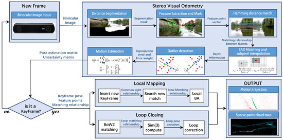
Figure 2.
Structure of the SP-SLAM system.
In the visual odometry thread, when a new stereo frame image is input, we first perform distance segmentation on the left image to obtain a mask that distinguishes between distant and near scenes. We then extract and label features from the stereo frame images. An improved stereo-matching method is used to measure the depth of feature points and calculate their 3D coordinates. During optimization and estimation, statistical methods are used to monitor outliers and adjust their weights, yielding preliminary estimation results.
Due to the continuous accumulation of tracking errors in the visual odometry thread, the system periodically uses additional information to correct the camera poses. To control memory usage during runtime, a KeyFrame strategy is employed to determine if a correction is needed based on specific conditions. We have improved the keyframe selection strategy by converting the estimated uncertainties into a scalar form for calculation and monitoring them using a sliding window.
In local mapping, we initialize keyframes and supplement co-visibility relationships. We update the depth information of map points based on new matching relationships. We optimize the poses and map points using the Huber loss function. Finally, we update all map points.
The loop closure follows the method of ORB-SLAM2, using Bag of Words (BoW) [36] for loop closure detection and Sim(3) for offset calculation and global correction.
3.1. Nearshore Feature Tracking
This section reviews the most critical aspect of our work: nearshore feature tracking. We extract features from stereo frame sequences for tracking and compute the camera’s 3D motion and its uncertainty by minimizing the reprojection error. A distance segmentation module is designed to extract and label feature points from different regions. We improve the depth measurement method by using SDA block matching and quadratic surface interpolation to obtain sub-pixel precision disparity, enabling accurate depth calculation of feature points. Additionally, we monitored and filtered outliers during optimization.
Through the analysis of stereo frame sequences, we identify the unique characteristics of feature points in nearshore environments. Due to the open nature of nearshore environments, the average depth is relatively large, and the depth measurement capability of stereo cameras is limited by their baseline length. Therefore, there is significant uncertainty in determining the depth of distant feature points. This uncertainty can adversely affect feature tracking between frames.
To address this issue, we implement a distance-based feature selection strategy, labeling feature points at different depths. In subsequent processing, we monitor and filter outliers among distant feature points to reduce their interference with motion estimation.
3.1.1. ORB Features
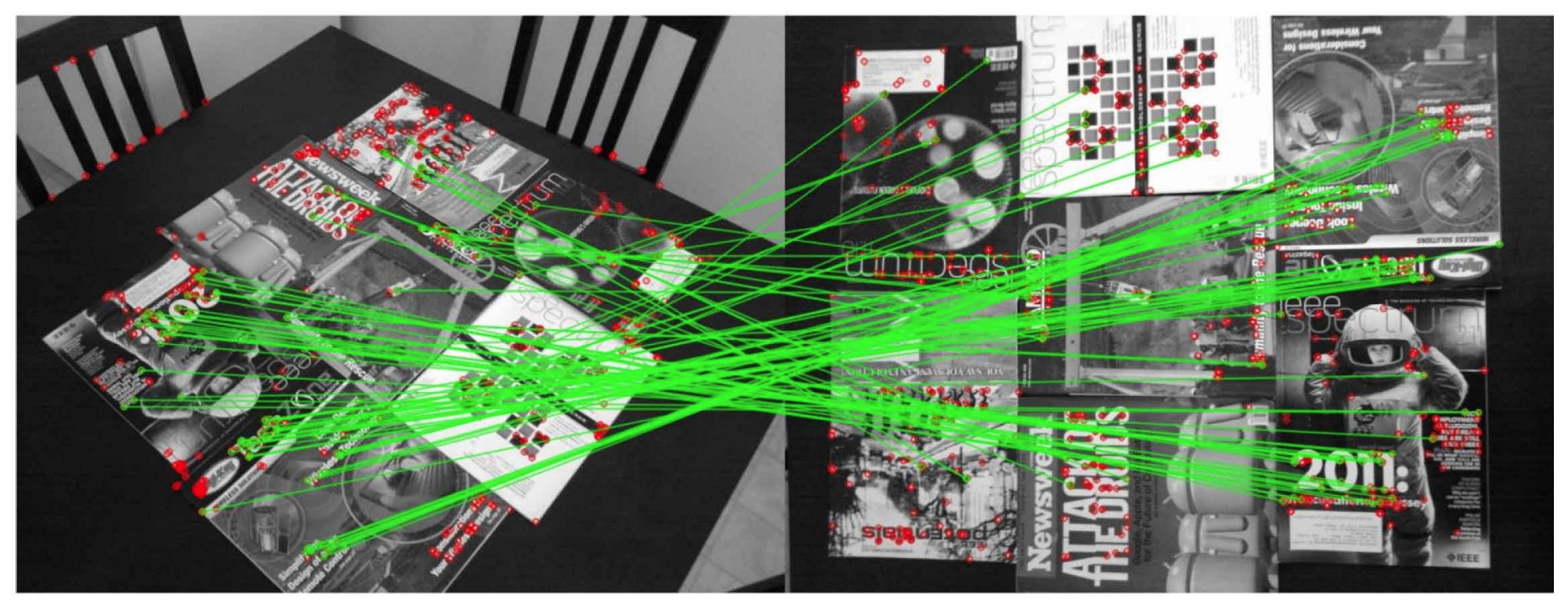
In this study, we continue to use ORB features [37] as the means for point feature extraction due to their excellent performance in keypoint detection. ORB employs oFAST keypoints, which are both rotation-invariant and scale-invariant, meeting the requirements for keypoint extraction in nearshore environments. Its strong rotational invariance (as shown in Figure 3) helps us track feature points under frequent viewpoint oscillations. For feature descriptors, we select BRIEF, a binary string that offers high extraction efficiency, high matching efficiency, and large information storage capacity.

Figure 3.
Rotation invariance and scale invariance of ORB features.
3.1.2. Distant Segmentation
To mitigate the impact of erroneous depth information from distant feature points on inter-frame feature tracking, we divide the image into distant and near regions and label the feature points in the distant region. Research on distance segmentation in open environments is not a mainstream field; most researchers [38] focus on using deep learning methods to estimate the depth of close-range images. Considering the limited computational resources of control equipment onboard small- to medium-sized USVs, deep learning, which requires a large number of parameters, may consume excessive computational resources and affect the results of localization calculations. Therefore, this study employs a traditional threshold-based segmentation method.
First, we determine whether the current frame contains distinct near and distant regions based on the pixel distribution of the image. For images that require segmentation, an initial coarse division is performed. Given that nearshore environment images may include areas such as the sky, where pixel intensities exhibit distinct characteristics, we calculate an appropriate threshold for preliminary segmentation.
The specific threshold selection uses the OTSU [39] method, which is based on the principle of maximizing inter-class variance. This method is suitable for images with a bimodal grayscale distribution, adaptively finding an appropriate threshold, as shown in Equation (1).
where and represent the proportions of the foreground and background, respectively, while and denote the mean gray values of the foreground and background, respectively. g is the inter-class variance. The algorithm traverses each gray value u and selects the gray value with the maximum inter-class variance as the segmentation threshold.
In the face of significant lighting variations in nearshore environments, images may experience sudden overexposure or low-light conditions. This can lead to inadequate segmentation. Therefore, we iteratively calculate the threshold while using a sliding window to monitor the pixel intensity histogram over a period of time, preventing abrupt changes in the threshold. Finally, we apply binarization to obtain a coarse delineation of the distant region, as shown in Equation (2).
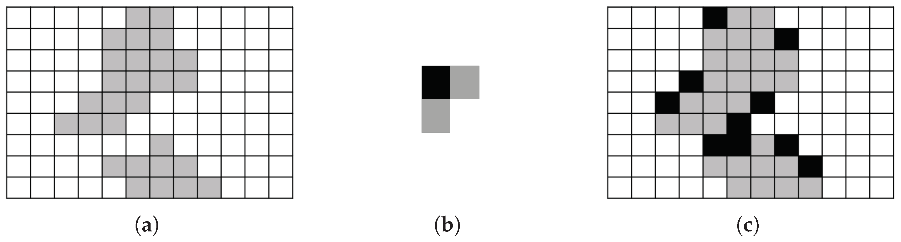
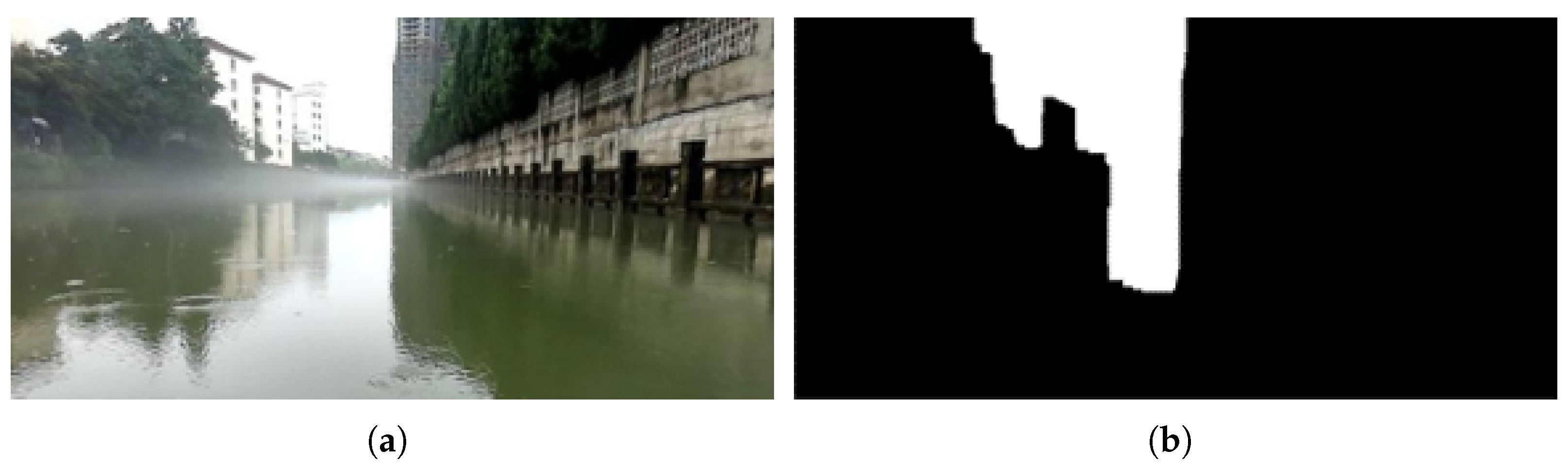
After the initial segmentation, a thorough segmentation of the distant regions in the image is performed. Morphological dilation operations are used to smooth the areas near the boundary lines. Dilation works by expanding the boundaries of the target region outward, filling small gaps and breaks by detecting changes in the pixels of the target area. The principle of dilation is illustrated in Figure 4. The specific effect is shown in Figure 5, where the white area in Figure 5b represents the distant area. The expanded image is segmented into the distant view of the nearshore environment, and the image distance segmentation function is realized.
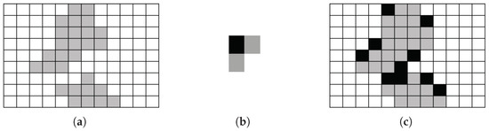
Figure 4.
Morphological dilatation, (a) is the original image, (b) is the structural element, and (c) is the expanded image; the gray areas represent the pixel distribution before dilation, while the black areas denote the pixels filled during the dilation process.

Figure 5.
Distance segmentation, (a) is the original image, (b) is the image after distance segmentation.
3.1.3. Stereo Calibration and Depth Estimation
Feature tracking estimates the motion increment between two frames by minimizing the reprojection error. This process requires obtaining the depth values of feature points relative to the camera. After extracting image features, we use SAD block matching and quadratic interpolation strategies to achieve sub-pixel precision disparity values, and then we calculate the depth of the feature points.
For disparity calculation, we adopt a “coarse matching—fine matching—sub-pixel interpolation” process. In epipolar line matching, we incorporate SAD block matching and quadratic surface interpolation techniques. During the coarse matching stage, we search along the camera’s epipolar line direction and match all feature points, identifying the best matching points. The matching index uses Hamming distance [40], as shown in Equation (3).
where and are the descriptors of two feature points, and ⊕ is the bitwise XOR operator.
In the depth-measurement process of ORB-SLAM2, linear window image block matching is used, achieving certain results. However, in nearshore environments, frequent viewpoint jitter causes the stereo camera baseline to fail to maintain a horizontal orientation. Therefore, we designed a square sliding window to expand the matching range and used the SAD method [41] to calculate the best matching neighborhood, obtaining the fine matching correction. This is expressed as follows in Equation (4):
where represents the start of the search window. is the value of the current offset location. denotes the minimum value in the search window. represents the values of the block to be matched. M and N represent the window search ranges along the -axis and -axis.
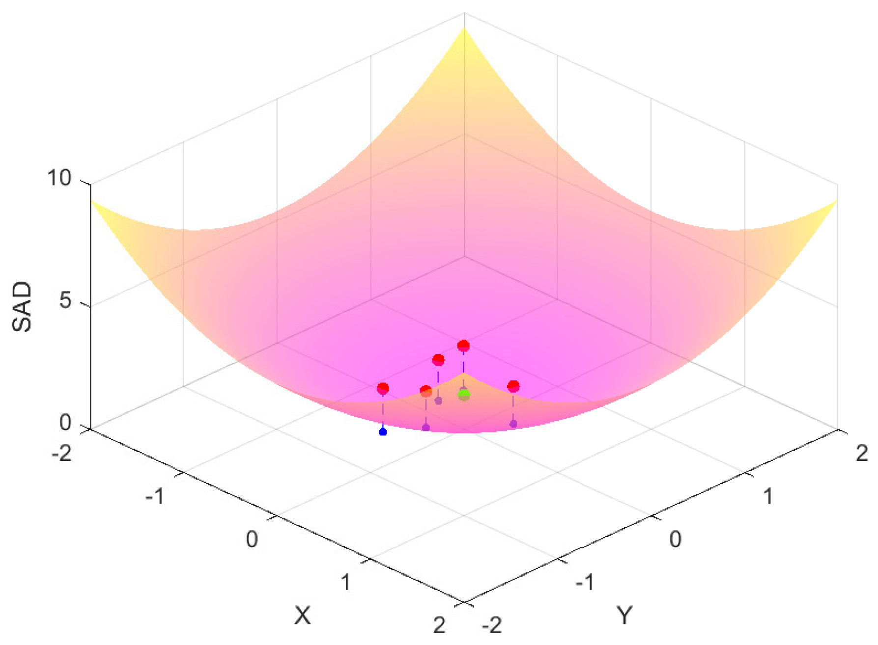
It is worth noting that the position of the best matching point does not necessarily coincide with a specific pixel location; thus, the disparity may result in sub-pixel accuracy. During the fine matching process, the similarity between image blocks within the sliding window and the image block near the feature point to be matched exhibits certain characteristics, forming a parabolic surface structure, as illustrated in Figure 6.

Figure 6.
Quadric interpolation diagram.
The establishment of this parabolic model requires only five sets of parameters. We use the best five sets of data from the fine matching process to construct the parabolic model and calculate the minimum value of the parabola. This value represents the local extremum within the sliding window, which is the optimal matching point. From the matching point, we obtain the sub-pixel level disparity and calculate the depth of the feature points using Equation (5).
where represents the depth value of the feature point, is the baseline length of the stereo camera, f is the focal length of the camera, and S is the disparity value of the feature point in the stereo frames.
3.1.4. Motion Estimation
During the process of motion estimation between two stereo frames, we utilize the minimization of projection error. Initially, we perform feature matching between frames to obtain a set of matched point pairs. In cases where multiple approximate matches exist, we directly filter them out to ensure that all matched points are sufficiently accurate.
We assume uniform motion of the camera and apply the motion increment from the previous frame to the camera extrinsic parameters of the current frame as the initial value for the optimization equation. The camera extrinsic parameters consist of a rotation matrix R and a translation vector t.
During the calculation of re-projection errors, the initial motion pose R and T are first applied to the set of 3D feature points extracted from the previous frame in the world coordinate system, transforming them into the current frame’s camera coordinate system. Subsequently, the camera intrinsic matrix K is used to project the 3D points in the camera coordinate system onto the image plane. The point set is then normalized according to the depth information. The projection process is described by Equation (6).
The reprojection error for all feature points is obtained by calculating the difference between the projected point set from the previous frame and the actual observed point set in the current frame. The difference is computed using the Euclidean distance, as shown in Equation (7).
We obtain the set of re-projection errors for the current frame and divide it into two parts based on the previously defined near-field and far-field regions: .
For the near-field region, which has high reliability, the errors are directly included in the total projection error. For the far-field region, where depth information is more prone to errors, we use the RANSAC method to filter outliers. A probabilistic model is then established based on the frequency of outlier occurrences to assess the uncertainty of the depth information for the current frame. When incorporating these errors into the total projection error, an adaptive weighting factor is applied based on the uncertainty, as shown in Equation (8).
After calculating the total re-projection error, an objective function is established based on this error, as shown in Equation (9). The optimal pose is obtained by minimizing the total re-projection error. We iteratively estimate the camera’s ego-motion using the Levenberg–Marquardt method.
Finally, we obtain the motion estimation between two consecutive frames and its uncertainty. This is represented in the form of a normal distribution: , where is the six-degree-of-freedom vector representing the camera motion between the previous and current frames, and represents the uncertainty covariance of this estimation. The covariance is approximated by computing the Hessian matrix from the error (represented by the Jacobian matrix) during the final iteration [18].
3.2. Local Mapping
This section primarily describes our work in the local mapping thread. To address the issue of tracking failures caused by frequent viewpoint jitter in nearshore environments. We have made three improvements in the mapping method.
1. We improve the keyframe selection strategy to convert the uncertainty of motion estimation into a scalar and constantly monitor it. Compared with traditional methods, it can insert keyframes in a more timely manner to correct accumulated errors.
2. We use the multi-view observation data of the same map point to update the depth information of the point, solve the problem of incorrect depth information in stereoscopic frame matching, and obtain a more accurate spatial position of the map point.
3. The pseudo-HUBER loss function is introduced in the local optimization of key frame attitude and map point position during mapping. This helps to filter outliers and improve the final map accuracy.
3.2.1. Keyframe Filtering and Initialization
During the feature tracking process, we continuously assess whether the current frame can be considered a keyframe. Once a new keyframe is confirmed, it is inserted into the SP-SLAM’s local mapping thread for further optimization. The selection of keyframes is based on the following three conditions, and meeting any one of these conditions is sufficient to insert a new keyframe:
1. A significant amount of time (number of frames) has passed since the last keyframe was generated, or sufficient movement has occurred, or of the feature points from the last keyframe have been lost.
2. The feature points of the previous frame have lost .
3. Using Equation (10), the uncertainty in each motion estimation is converted from the Hessian matrix to a scalar [42].
where m denotes the dimensionality of the covariance matrix representing the uncertainty. We then employ a sliding window to monitor the changes in uncertainty across several pose estimations. If the rate of change exceeds , it indicates an unstable state, necessitating the insertion of a keyframe.
When a new keyframe is added to the local mapping thread, we obtain the camera pose of the new keyframe, the 3D positions of the feature points in the world coordinate system, and their matching relationships. We then perform new matching within the existing keyframe database and optimize both the pose and the map points.
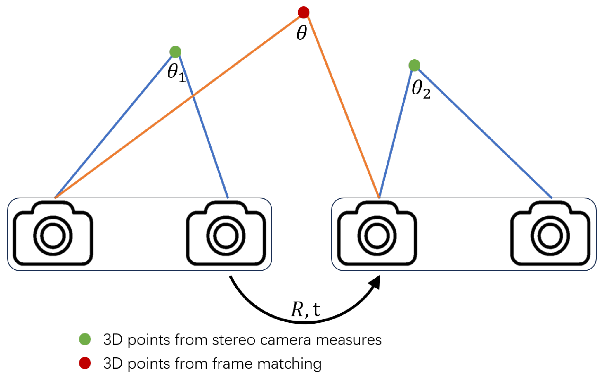
During feature tracking, the 3D reconstruction of feature points relies entirely on stereo frame matching for depth measurement, which is prone to significant errors. Therefore, when a new keyframe is inserted, we update the 3D coordinates of the feature points. For feature points in the new keyframe that have matching relationships in other keyframes, referred to as co-visibility, we re-triangulate these feature points using the co-visible keyframes. As illustrated in Figure 7, when the depth value deviates significantly or exhibits anomalies during RANSAC detection when or the depth values exhibit anomalies during RANSAC detection, the 3D points are updated using triangulation between the co-visible keyframes (red lines); otherwise, the old values are used.
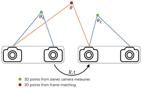
Figure 7.
Three-dimensional point updating.
3.2.2. Local Bundle Adjustment
Local Bundle Adjustment (BA) is a commonly used method to improve the accuracy of the local map. This method is based on the fundamental idea of minimizing reprojection error. By optimizing the camera poses and the positions of map points within the local region, it iteratively computes more accurate values using additional constraint relationships.
Unlike the feature tracking stage, the goal of local Bundle Adjustment (BA) is to minimize the reprojection error of all observed points by simultaneously adjusting camera poses and map point positions. The reprojection error is defined as follows:
where is the observed position (pixel coordinates) of the map point in keyframe . is the computed result of projecting the map point onto the image plane using the camera projection model and the pose of keyframe .
Since we re-measured the positions of map points during keyframe initialization, all errors are assigned uniform weights in the local BA process. The objective function for local BA is established as follows:
We continue to use the Levenberg–Marquardt method for iterative optimization. Additionally, we refer to the method proposed in [43], employing a pseudo-Huber loss function to handle outliers and ensure data reliability.
4. Experiment
To evaluate the performance of the proposed SP-SLAM, we conducted experiments on the USVInland Dataset [44], which is designed for surface environments. USVInland is the first multi-sensor dataset specifically for USVs in inland waterways. This dataset is provided by ORCAUBOAT, located in Xi’an, China. We obtained access to six sequences from the USVInland dataset through a research process.
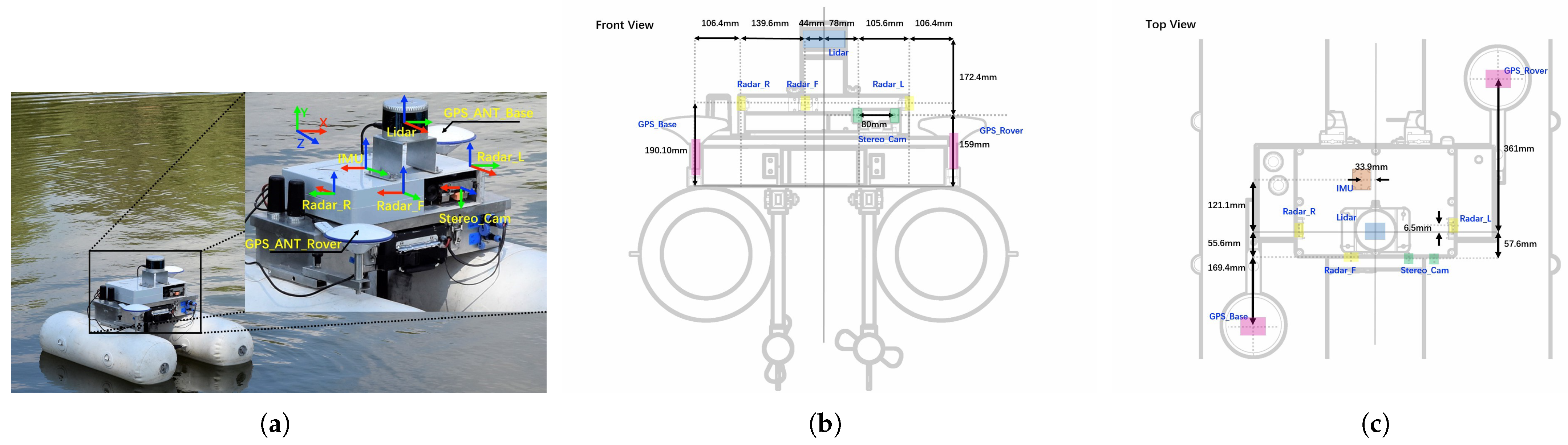
USVInland utilizes USVs to record navigation data in inland waterways. The sensor layout on the USVs is shown in Figure 8. Three IWR684 millimeter-wave radars from Texas Instruments are mounted on the sides and front of the ship, recording information along the shoreline and detecting obstacles ahead. A 16-line LiDAR from LeiShen Intelligence System Co., Ltd., Shenzhen, China, was installed on the top of the boat to record point cloud information along the shore, capable of capturing environmental data up to a depth of 100 m. A stereo camera with a baseline length of 8 cm is installed to record visual information during navigation. The data collected by this device are also the most critical for SP-SLAM. An IMU (Inertial Measurement Unit) is mounted at the center of gravity of the vessel to record the vessel’s attitude and acceleration.
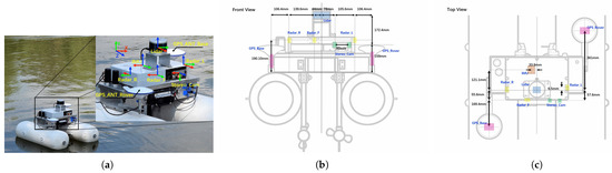
Figure 8.
USVInland Acquisition Platform: (a) is the physical picture of the unmanned ship, (b) is the front view of the unmanned ship, (c) is the top view of the unmanned ship.
In addition, a GPS positioning system with RTK technology is used to record the real-time trajectory of the vessel. However, due to several GPS signal-blocked waterways encountered during navigation, these data are for reference only.
The USVInland dataset encompasses various weather conditions such as sunny days, rainy days, and heavy fog. These sequences capture visual information at different distances from the shore, including vegetation, boats, and shore-based structures. The travel distances in each sequence range from 70 m to 400 m.
In the experimental section, we first conducted experiments on the effectiveness of distant segmentation. Different morphological operation structures were used to experiment on nearshore environment images under various conditions. For the overall evaluation of the SLAM system, we performed a qualitative analysis of motion trajectories, a comparison of absolute trajectory errors, a comparison of relative trajectory errors, and a qualitative comparison of mapping results.
Apart from the USVInland dataset, we also utilized the widely used standard dataset KITTI [45] for evaluating the SP-SLAM system in the field of autonomous driving. The KITTI dataset consists of 11 sequences, all of which were collected from urban road information by moving vehicles. These urban road scenes also include factors from open areas. Our method is capable of segmenting and extracting information from these features.
All experiments were conducted on a personal computer equipped with an Intel Core i7-12700 CPU and 32GB RAM, running Ubuntu 20.04 operating system.
4.1. Distant Segmentation and Experiment
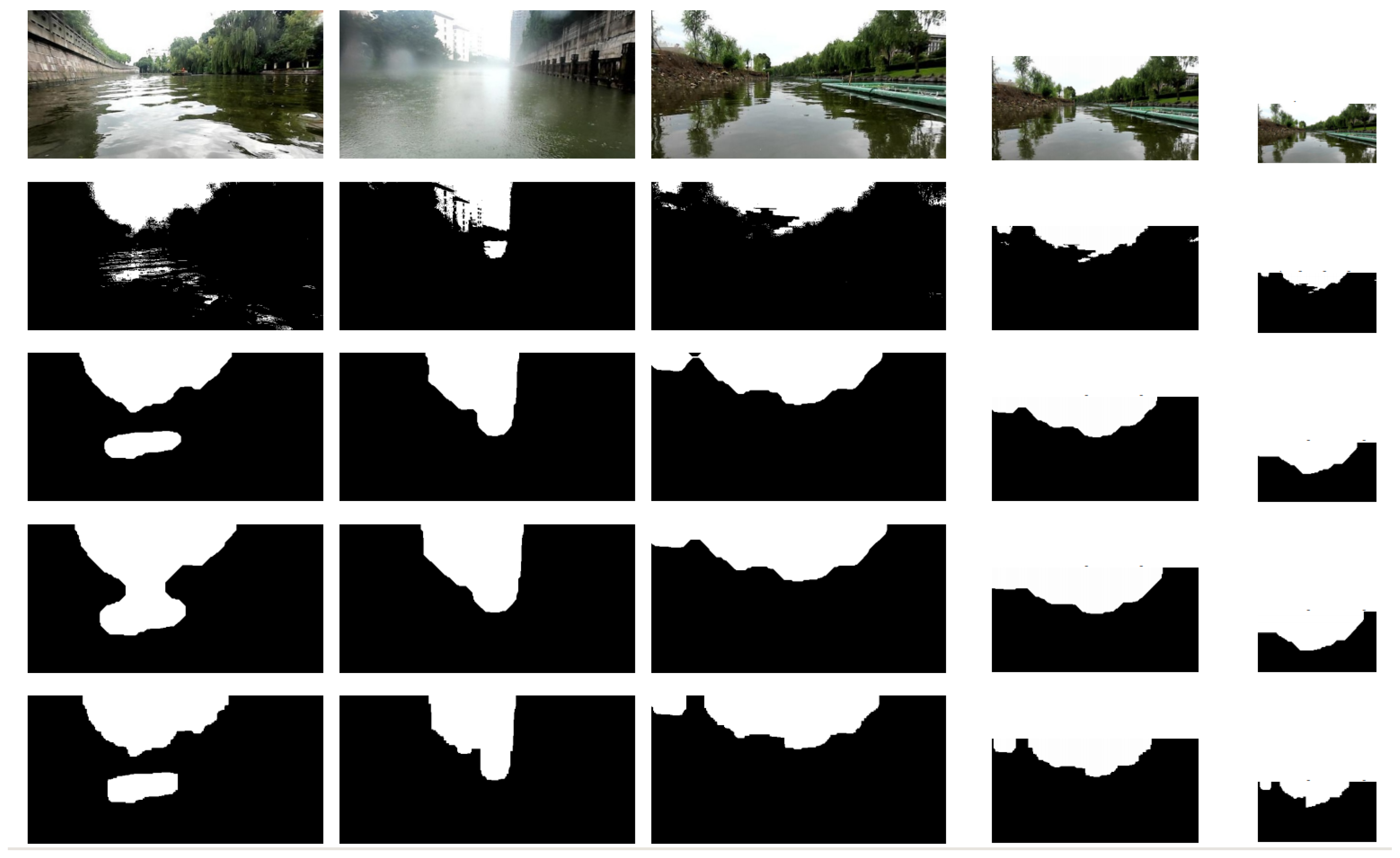
During the experiments, we first calculated the threshold iteratively and used binarization to achieve initial distance segmentation, as shown in the second row in Figure 9. Subsequently, we selected the two largest connected regions in the distant part of the image and applied dilation operations using different structural elements on these two regions to obtain the final distant and near-scene segmentation results.

Figure 9.
The distance segmentation effect processed by different structural parts is as follows: the first act is the original image, the second act is the binary image segmented by the iterative threshold, and the third to fifth lines are segmented by different structural elements.
The experiment tested images of nearshore environments under different weather conditions and scales. The first column of Figure 9 depicts cloudy weather, the second column depicts rainy weather, the third column depicts sunny weather, and the fourth and fifth columns depict sunny weather images scaled down by factors of 2 and 4.2, respectively. We utilized different structuring elements and analyzed their impact on the segmentation results. In the third row of sub-images, a circular structuring element with a radius of 15 pixels was used. In the fourth row, a circular structuring element with a radius of 25 pixels was employed. In the fifth row, a rectangular structuring element with a length of 25 pixels and a width of 15 pixels was applied.
The experimental results indicate that circular structuring elements produce smoother edges in the segmentation of near- and far-field scenes, while rectangular structuring elements are more advantageous in expanding and supplementing connected regions. Considering the fundamental requirements for near and far-field segmentation in nearshore visual localization, we ultimately chose to use a circular structuring element with a radius of 25 pixels.
After distance segmentation, performing feature extraction on the image can effectively identify distant points, reducing the impact of erroneous depth values from these points on pose estimation. As shown in Figure 10a, the proposed method extracts most of the distant points in areas very close to the shore. In Figure 10b, the method also successfully segments the distant building regions as far-field in rainy and foggy weather. In the open large-scale scenes depicted in Figure 10c,d, this method successfully segments the far-field regions and marks the majority of distant feature points. Notably, in Figure 10d, when confronted with a similarly white sky and wall, the method successfully marks the feature points at the boundary between the distant area and the sky, thereby avoiding the large, light-colored areas near the white wall in the foreground.
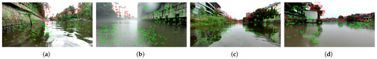
Figure 10.
Nearshore feature extraction effect, (a–d) illustrate the extraction results in different scenarios, where the green points represent foreground feature points and the red points represent background feature points.
4.2. Comparison of Motion Trajectories
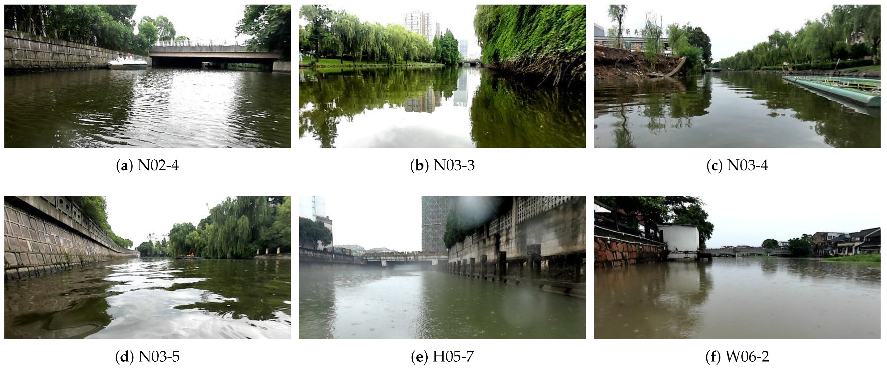
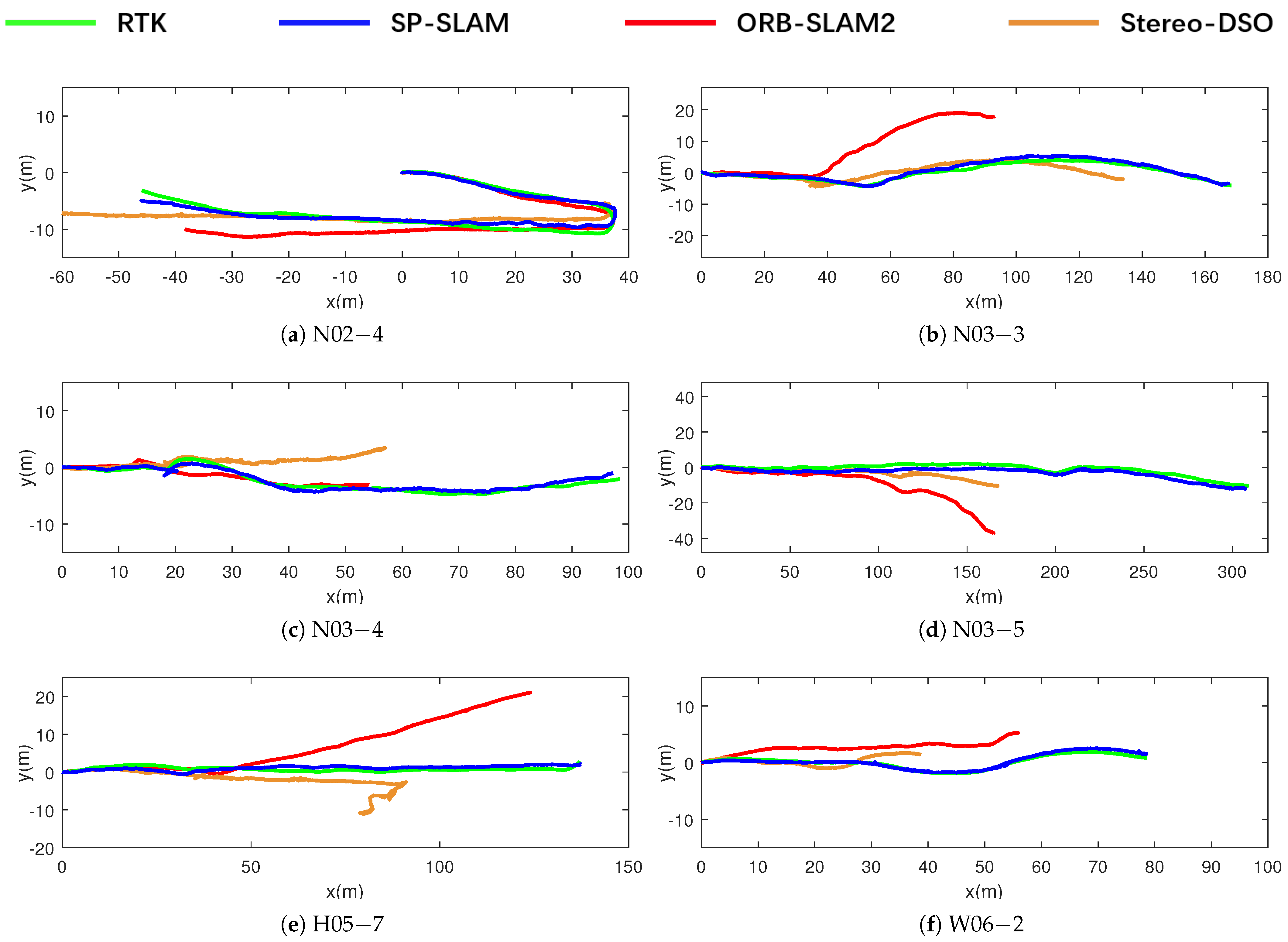
To visually demonstrate the effectiveness of the SP-SLAM algorithm, this paper uses the RTK-collected data from the USVInland dataset as the ground truth trajectory. We plot the output trajectories of the feature-based ORB-SLAM2 algorithm, the direct method-based Stereo-DSO [46] algorithm, and our proposed algorithm. These trajectories are visualized together for qualitative comparison. Figure 11 shows the specific scenes of six different sequences. The six sequences have certain differences in weather conditions, traveling distance, and round-trip conditions. The comparison of the algorithm running trajectory is shown in Figure 12.

Figure 11.
USVInland real environment presentation.
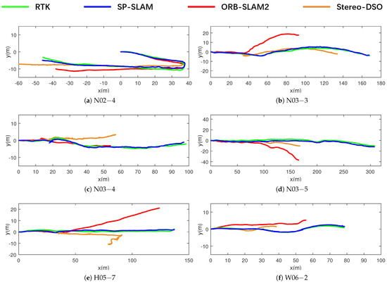
Figure 12.
Comparison of motion trajectories.
In the N02-4 sequence, which includes a significant rotational movement and a bridge scene, SP-SLAM maintains better accuracy, whereas ORB-SLAM2 and Stereo-DSO, influenced by various factors, incorrectly estimate the travel distance. The N03-3 sequence involves navigation along the shoreline vegetation, with distant buildings and other difficult-to-measure depth information. SP-SLAM accurately reconstructs this trajectory. The N03-4 sequence follows a river channel, where there are some simultaneously moving vessels on the water surface, posing a significant challenge for feature tracking and causing some degradation during motion. Stereo-DSO’s estimation of both scale and rotation is affected, but SP-SLAM still accurately reconstructs the motion trajectory.
In the N03-5, H05-6, and W06-2 sequences, the traditional ORB-SLAM2 algorithm incorrectly estimates depth. The performance of the direct method-based Stereo-DSO in these sequences is poor, even leading to tracking loss in some cases. Thanks to the distance segmentation method used in SP-SLAM, we reduce the impact of these erroneous depths on the final results, achieving more accurate outcomes.
From the comparative trajectory plots of the above sequences, it can be observed that the traditional ORB-SLAM2 method performs well in tracking rotational movements, accurately reconstructing both small turns and large rotations in the true trajectory. However, it fails to restore the correct scale during translational movements in pose tracking. The direct method-based Stereo-DSO struggles to reconstruct the pose accurately due to complex lighting variations on the water surface. In contrast, the proposed SP-SLAM effectively restores the scale, resulting in a more accurate trajectory.
4.3. Absolute Trajectory Error Comparison
For a precise comparison of motion trajectory errors, we use Absolute Trajectory Error (ATE). The ATE calculation estimates the difference between the estimated trajectory and the ground truth trajectory, directly reflecting the SLAM algorithm’s localization accuracy and global trajectory consistency. The ATE values for the two algorithms across six sequences in the USVInland dataset are shown in Table 1.

Table 1.
Comparisons of ATE [m] in dynamic sequences of USVInland dataset for ORB-SLAM2 and SP-SLAM.
According to Table 1, the ATE estimated by our SP-SLAM algorithm is superior to that of the traditional ORB-SLAM2 algorithm across all six data sequences. The accuracy of camera pose estimation has significantly improved, with a notable reduction in absolute trajectory error, indicating preliminary localization capability. The traditional ORB-SLAM2 algorithm’s incorrect scale estimation results in substantial trajectory error, rendering it ineffective for motion estimation and localization. This finding is consistent with the results obtained by the developers of the USVInland dataset.
4.4. Relative Pose Error Comparison
In addition to the precise data comparison of motion trajectory errors, we also calculate the Relative Pose Error (RPE) for both algorithms. RPE measures the difference between the estimated pose change and the true pose change over a fixed time interval, reflecting the local localization accuracy of the SLAM algorithm. We divide RPE into rotational error and translational error for separate calculations to more intuitively demonstrate the advantages of the SP-SLAM algorithm.
The RPE values for both algorithms across six sequences in the USVInland dataset are shown in Table 2 and Table 3. Table 2 presents the translational errors, where SP-SLAM achieves significant improvements in frame-to-frame translational estimation compared to ORB-SLAM2, with each frame’s translational estimate being more accurate. Table 3 shows the rotational estimates, indicating that both ORB-SLAM2 and SP-SLAM perform well in rotational estimation. By improving keyframe selection, SP-SLAM achieves better rotational accuracy. However, in the N03-4 sequence, SP-SLAM encounters an erroneous estimation, incorrectly determining that the vessel has reversed direction. Nonetheless, the system automatically optimizes and corrects this error in the subsequent keyframes, ensuring the accuracy of the trajectory.
Table 2.
Comparisons of RPE [m/s] in dynamic sequences of USVInland dataset for ORB-SLAM2 and SP-SLAM.
Table 3.
Comparisons of RPE [deg/s] in dynamic sequences of USVInland dataset for ORB-SLAM2 and SP-SLAM.
4.5. Algorithm Efficiency Analysis
To verify the impact of adding a distance segmentation module and improving the depth estimation algorithm, we collect and analyze the processing time of each image frame. Each image extracts 1500 feature points, and comparative tests were conducted on a personal computer (Intel Core i7-12700 4.90 GHz CPU, 32 GB RAM, and Ubuntu 20.04) and a commonly used embedded platform, Jetson Nano (4 GB RAM). The specific results are shown in Table 4 and Table 5.
Table 4.
Inference speed on personal computer (ms).
Table 5.
Inference speed on Jetson nano (ms).
It can be observed that the method proposed in this paper takes more time in the feature tracking thread compared to the traditional ORB-SLAM2. This is due to the additional computational load introduced by the distance segmentation module, quadratic surface interpolation method, and the computation of the Hessian matrix representing uncertainty during optimization. However, SP-SLAM is still able to maintain a frame rate of around 8 FPS on embedded devices, which basically meets the real-time localization requirements of unmanned surface vessels.
4.6. KITTI Dataset Error Comparison
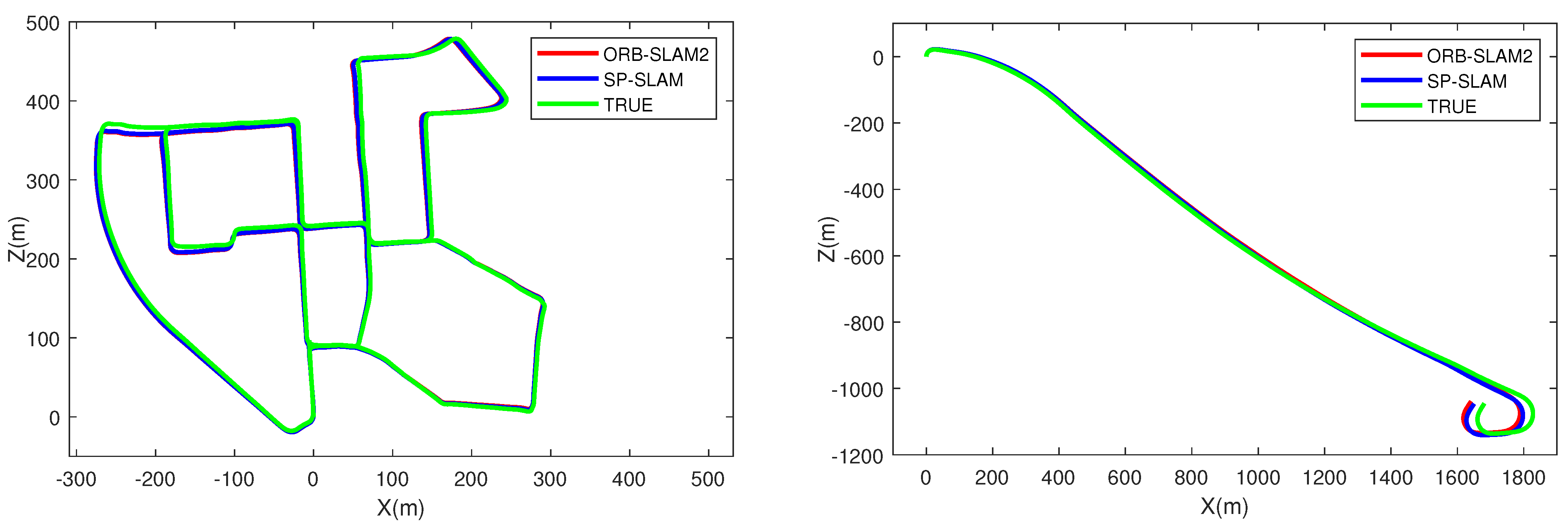
We also conduct a comparison of the KITTI dataset with the traditional ORB-SLAM2 and the direct method-based stereo DSO, using ATE and RPE as evaluation metrics. As shown in Table 6, we divide RPE into angular relative error and translation relative error , and ATE only compares the absolute error of translation . SP-SLAM’s performance is generally on par with the classic methods across various sequences and shows certain improvements in large-scale scenes. We also present the trajectory comparison plots for the 00 and 01 sequences in the KITTI dataset, as shown in Figure 13. It can be observed that the approach of filtering out feature points with anomalous depth values in SP-SLAM does not introduce system bias. Overall, the performance shows a slight improvement compared to the traditional ORB-SLAM2 (stereo) and Stereo-DSO.
Table 6.
Comparisons of RPE and ATE of KITTI dataset for ORB-SLAM2 and SP-SLAM.
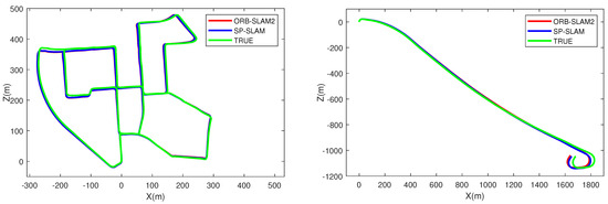
Figure 13.
KITTI datasets 00, 01 sequence trajectory comparison diagram.
4.7. Qualitative Analysis of Mapping Effect
To verify the actual mapping performance of SP-SLAM in nearshore environments, we qualitatively analyze the mapping results of two sequences. The SP-SLAM algorithm proposed in this paper is a sparse feature point SLAM algorithm; therefore, we do not impose overly stringent requirements on the mapping results. The primary goal is to roughly depict the surrounding scene and provide localization results.
Figure 14 shows the mapping results for the N03-5 sequence, which involves navigation along a shoreline. Figure 14a displays the actual environment of the shoreline and the mapping effect for this section. The algorithm successfully extracts feature information from the stones and brick seams, accurately reconstructing the positions of feature points from near to far in three-dimensional space, thereby reflecting the spatial relationships between the feature points. Figure 14b provides a satellite overhead view of the data collection area for this sequence and the overall mapping results for the area. The approximate motion path is marked by a red line. The mapping thread constructs the entire shoreline along the path without significant overlap or degradation phenomena.
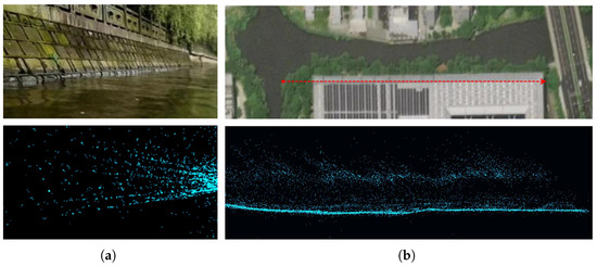
Figure 14.
N03-5 mapping effect display, (a) shows the real scene image and mapping results of the riverbanks, and (b) displays the satellite top view of the river and the overall mapping outcomes. The red line in the figure indicates the approximate path of the unmanned surface vessel.
Figure 15 shows the mapping results for the N02-4 sequence, which includes a 180-degree rotation and captures bridge scenes from two different directions in the nearshore environment. Figure 15a presents the bridge scenes in both directions before and after the rotation. Figure 15b provides a satellite overhead view and the overall mapping results for the area. Notably, as the sequence moves under the bridge, the information observed after the rotation (the right side of the point cloud in Figure 15b) is roughly constructed in the map. Additionally, no excessive spatial point drift occurs during the mapping process.
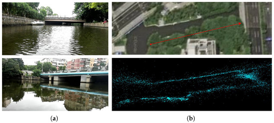
Figure 15.
N02-4 mapping effect display, (a) shows the real scene images of both ends of the river, both of which are bridge scenes; (b) displays the satellite top view of the river and the overall mapping results. The red line in the figure indicates the approximate path of the USVs.
Additionally, the primary limitation of our mapping method lies in the granularity of the maps produced. In current autonomous driving systems, perception typically constructs more detailed and fine-grained maps by using mapping techniques. However, the method described in this paper follows the ORB-SLAM2 mapping strategy, which produces a sparse point cloud map. The main reason for this approach is that the main control computer resources of the unmanned vessel we plan to produce are limited, and constructing detailed maps would consume a significant amount of memory resources.
5. Conclusions
In this study, we propose a stereo vision SP-SLAM system employing a distance segmentation strategy for nearshore water surface environments. The focus is on addressing the impact of erroneous feature depths on motion estimation within nearshore environments. We incorporate a distance segmentation method into the visual odometry thread to label feature information across different regions. During the optimization process, we monitor and filter out feature points with abnormal depth values to mitigate the influence of erroneous depth information on pose estimation results. We have improved the binocular depth measurement method, enhancing the accuracy of feature point measurements and obtaining more precise map information.
SP-SLAM is a SLAM system specifically designed for water surface scenarios, and we conducted experiments using the USVInland dataset. Experimental results verify that our algorithm effectively addresses motion estimation errors caused by erroneous depth information, thereby enhancing the robustness of the algorithm. We performed real-time tests on an embedded system, demonstrating that it can construct sparse point cloud maps for localization, essentially restoring image features.
We believe that the SP-SLAM localization and mapping method proposed in this paper can provide real-time environmental information for the planning and control of unmanned surface vessels in nearshore environments. This enables features such as adaptive cruising and emergency braking. Additionally, it allows for advanced route planning to avoid obstacles and terrain in the environment. According to the relevant autonomous driving classification manual [47], we believe that, with the support of the method presented in this paper, the unmanned surface vessel can achieve Level 2 autonomous driving.
Compared to the previously mentioned AHV [12], our method improves the average accuracy and achieves positioning under conditions where GPS signals are obstructed. The visual algorithm in this paper can also perform object recognition and localization functions, enabling it to undertake more nearshore tasks.
However, there is still significant room for improvement in current positioning accuracy. SP-SLAM, while effective, has certain deficiencies when operating in nearshore environments. It struggles to accurately track feature points amidst water ripples. We plan to incorporate deep learning techniques to achieve more accurate matching. Additionally, the issue of viewpoint jitter caused by water flow impacts in nearshore environments also affects the algorithm’s accuracy. We believe this problem can be mitigated by introducing an inertial navigation module. By constructing a tightly coupled multi-sensor fusion framework, we can compensate for variations in viewpoint.
Apart from these existing challenges for navigation planning and control of USVs, we believe that combining nearshore environment visual localization with traditional satellite-based positioning can be beneficial. Furthermore, employing multi-layered planning and control strategies from the field of autonomous driving, such as the MAS-Based Hierarchical Architecture developed by Liang et al. [48], can effectively address the tasks of tracking, prediction, and control during the navigation of the USVs. This approach aims to achieve full-process autonomous navigation capabilities for USVs.
Author Contributions
Data curation, X.L.; methodology, X.G., X.L. and F.L.; writing—original draft preparation, X.L.; writing—review and editing, F.L. and H.H; funding acquisition, H.H. All authors have read and agreed to the published version of the manuscript.
Funding
This work was supported by the Education and Scientific Research Project of Fujian Provincial Department of Finance (Grant GY-Z23272 and GY-Z23010), key scientific and technological innovation projects of Fujian Province: 2023XQ015, and the Research start-up funding of The Fujian University of techology: GY-Z23056.
Data Availability Statement
Data are contained within the article.
Acknowledgments
Thank you to the ORCAUBOAT Company for providing USVInland dataset support for this paper.
Conflicts of Interest
The authors declare that they have no known competing financial interests or personal relationships that could have appeared to influence the work reported in this paper.
References
- Heo, J.; Kim, J.; Kwon, Y. Analysis of design directions for unmanned surface vehicles (USVs). J. Comput. Commun. 2017, 5, 92–100. [Google Scholar] [CrossRef]
- Peng, Y.; Yang, Y.; Cui, J.; Li, X.; Pu, H.; Gu, J.; Xie, S.; Luo, J. Development of the USV ‘JingHai-I’ and sea trials in the Southern Yellow Sea. Ocean. Eng. 2017, 131, 186–196. [Google Scholar] [CrossRef]
- Barrera, C.; Padron, I.; Luis, F.S.; Llinas, O. Trends and challenges in unmanned surface vehicles (USV): From survey to shipping. TransNav Int. J. Mar. Navig. Saf. Sea Transp. 2021, 15, 135–142. [Google Scholar] [CrossRef]
- Wang, Y.; Liu, W.; Liu, J.; Sun, C. Cooperative USV–UAV marine search and rescue with visual navigation and reinforcement learning-based control. ISA Trans. 2023, 137, 222–235. [Google Scholar] [CrossRef] [PubMed]
- Makar, A. Coastal bathymetric sounding in very shallow water using USV: Study of public beach in Gdynia, Poland. Sensors 2023, 23, 4215. [Google Scholar] [CrossRef] [PubMed]
- Specht, O. Land and Seabed Surface Modelling in the Coastal Zone Using UAV/USV-Based Data Integration. Sensors 2023, 23, 8020. [Google Scholar] [CrossRef] [PubMed]
- Makar, A. Limitations of Multi-GNSS Positioning of USV in Area with High Harbour Infrastructure. Electronics 2023, 12, 697. [Google Scholar] [CrossRef]
- Tetreault, B.J. Use of the Automatic Identification System (AIS) for maritime domain awareness (MDA). In Proceedings of the Oceans 2005 MTS/IEEE, Washington, DC, USA, 17–23 September 2005; pp. 1590–1594. [Google Scholar]
- Ma, H.; Smart, E.; Ahmed, A.; Brown, D. Radar image-based positioning for USV under GPS denial environment. IEEE Trans. Intell. Transp. Syst. 2017, 19, 72–80. [Google Scholar] [CrossRef]
- Han, J.; Cho, Y.; Kim, J. Coastal SLAM with marine radar for USV operation in GPS-restricted situations. IEEE J. Ocean. Eng. 2019, 44, 300–309. [Google Scholar] [CrossRef]
- Liu, W.; Liu, Y.; Bucknall, R. A robust localization method for unmanned surface vehicle (USV) navigation using fuzzy adaptive Kalman filtering. IEEE Access 2019, 7, 46071–46083. [Google Scholar] [CrossRef]
- Broman, D.R.; Ledesma, M.M.; Pujol, B.G.; Díaz, A.A.; Subirana, J.T. A Low-Cost Autonomous Vehicles for Coastal Sea Monitoring; Mediterranean Institute of Advanced Studies (CSIC–UIB): Esporles, Spain, 2005. [Google Scholar]
- Nistér, D.; Naroditsky, O.; Bergen, J. Visual odometry. In Proceedings of the 2004 IEEE Computer Society Conference on Computer Vision and Pattern Recognition 2004, Washington, DC, USA, 27 June–2 July 2004; Volume 1. [Google Scholar]
- Taketomi, T.; Uchiyama, H.; Ikeda, S. Visual SLAM algorithms: A survey from 2010 to 2016. IPSJ Trans. Comput. Vis. Appl. 2017, 9, 16. [Google Scholar] [CrossRef]
- Nistér, D. Preemptive RANSAC for live structure and motion estimation. Mach. Vis. Appl. 2005, 16, 321–329. [Google Scholar] [CrossRef]
- Trujillo, J.-C.; Cano-Izquierdo, J.M.; de la Escalera, A.; Armingol, J.-M. Cooperative Visual-SLAM System for UAV-Based Target Tracking in GPS-Denied Environments: A Target-Centric Approach. Electronics 2020, 9, 813. [Google Scholar] [CrossRef]
- Mur-Artal, R.; Tardós, J.D. Orb-slam2: An open-source slam system for monocular, stereo, and rgb-d cameras. IEEE Trans. Robot. 2017, 33, 1255–1262. [Google Scholar] [CrossRef]
- Gomez-Ojeda, R.; Moreno, F.A.; Zuniga-Noël, D.; Scaramuzza, D.; Gonzalez-Jimenez, J. PL-SLAM: A stereo SLAM system through the combination of points and line segments. IEEE Trans. Robot. 2019, 35, 734–746. [Google Scholar] [CrossRef]
- Liang, J.; Tian, Q.; Feng, J.; Pi, D.; Yin, G. A polytopic model-based robust predictive control scheme for path tracking of autonomous vehicles. IEEE Trans. Intell. Veh. 2023, 9, 3928–3939. [Google Scholar] [CrossRef]
- Newcombe, R.A.; Lovegrove, S.J.; Davison, A.J. DTAM: Dense tracking and mapping in real-time. In Proceedings of the 2011 International Conference on Computer Vision, Barcelona, Spain, 6–13 November 2011. [Google Scholar]
- Engel, J.; Schöps, T.; Cremers, D. LSD-SLAM: Large-scale direct monocular SLAM. In Proceedings of the European Conference on Computer Vision, Zurich, Switzerland, 6–12 September 2014; Springer International Publishing: Cham, Switzerland, 2014. [Google Scholar]
- Forster, C.; Pizzoli, M.; Scaramuzza, D. SVO: Fast semi-direct monocular visual odometry. In Proceedings of the 2014 IEEE International Conference on Robotics and Automation (ICRA), Hong Kong, China, 31 May–7 June 2014; pp. 15–22. [Google Scholar]
- Pire, T.; Fischer, T.; Castro, G.; De Cristóforis, P.; Civera, J.; Berlles, J.J. S-PTAM: Stereo parallel tracking and mapping. Robot. Auton. Syst. 2017, 93, 27–42. [Google Scholar] [CrossRef]
- Mur-Artal, R.; Martinez Montiel, J.M.; Tardos, J.D. ORB-SLAM: A versatile and accurate monocular SLAM system. IEEE Trans. Robot. 2015, 31, 1147–1163. [Google Scholar] [CrossRef]
- Li, P.; Cao, C. Vision SLAM Algorithm for Low Light Environment. J. Beijing Univ. Posts Telecommun. 2024, 47, 106. [Google Scholar]
- Tian, L.; Yan, Y.; Li, H. SVD-SLAM: Stereo Visual SLAM Algorithm Based on Dynamic Feature Filtering for Autonomous Driving. Electronics 2023, 12, 1883. [Google Scholar] [CrossRef]
- Ai, Y.; Wang, L.; Liu, Q.; Zhang, M.; Fang, H. Stereo SLAM in Dynamic Environments Using Semantic Segmentation. Electronics 2023, 12, 3112. [Google Scholar] [CrossRef]
- Guo, D.; Li, K.; Hu, B.; Zhang, Y.; Wang, M. Benchmarking Micro-action Recognition: Dataset, Methods, and Applications. IEEE Trans. Circuits Syst. Video Technol. 2024, 34, 6238–6252. [Google Scholar] [CrossRef]
- Wei, Y.; Xi, Y. Optimization of 3-D pose measurement method based on binocular vision. IEEE Trans. Instrum. Meas. 2022, 71, 8501312. [Google Scholar] [CrossRef]
- Kuppala, K.; Banda, S.; Barige, T.R. An overview of deep learning methods for image registration with focus on feature-based approaches. Int. J. Image Data Fusion 2020, 11, 113–135. [Google Scholar] [CrossRef]
- Lin, H.; Tsai, C. Depth measurement based on stereo vision with integrated camera rotation. IEEE Trans. Instrum. Meas. 2021, 70, 5009210. [Google Scholar] [CrossRef]
- Zou, X.; Gao, J.; Li, H.; Zhang, Y.; Liu, F.; Wu, H.; Yao, R. Novel Visual Odometry Method for Water Autonomous Navigation. In Proceedings of the 2022 2nd International Conference on Computation, Communication and Engineering (ICCCE), Guangzhou, China, 4–6 November 2022; pp. 13–17. [Google Scholar]
- Zou, X.; Zhan, W.; Xiao, C.; Zhou, C.; Chen, Q.; Yang, T.; Liu, X. A novel vision-based towing angle estimation for maritime towing operations. J. Mar. Sci. Eng. 2020, 8, 356. [Google Scholar] [CrossRef]
- Volden, Ø.; Cabecinhas, D.; Pascoal, A.; Fossen, T.I. Development and experimental evaluation of visual-acoustic navigation for safe maneuvering of unmanned surface vehicles in harbor and waterway areas. Ocean. Eng. 2023, 280, 114675. [Google Scholar] [CrossRef]
- Cortes-Vega, D.; Alazki, H.; Rullan-Lara, J.L. Visual odometry-based robust control for an unmanned surface vehicle under waves and currents in a urban waterway. J. Mar. Sci. Eng. 2023, 11, 515. [Google Scholar] [CrossRef]
- Gálvez-López, D.; Tardos, J.D. Bags of binary words for fast place recognition in image sequences. IEEE Trans. Robot. 2012, 28, 1188–1197. [Google Scholar] [CrossRef]
- Rublee, E.; Rabaud, V.; Konolige, K.; Bradski, G. ORB: An efficient alternative to SIFT or SURF. In Proceedings of the 2011 International Conference on Computer Vision, Barcelona, Spain, 6–13 November 2011. [Google Scholar]
- Ming, Y.; Meng, X.; Fan, C.; Yu, H. Deep learning for monocular depth estimation: A review. Neurocomputing 2021, 438, 14–33. [Google Scholar] [CrossRef]
- Xu, X.; Xu, S.; Jin, L.; Song, E. Characteristic analysis of Otsu threshold and its applications. Pattern Recognit. Lett. 2011, 32, 956–961. [Google Scholar] [CrossRef]
- Hamming, R.W. Error detecting and error correcting codes. Bell Syst. Tech. J. 1950, 29, 147–160. [Google Scholar] [CrossRef]
- Vanne, J.; Aho, E.; Hamalainen, T.D.; Kuusilinna, K. A high-performance sum of absolute difference implementation for motion estimation. IEEE Trans. Circuits Syst. Video Technol. 2006, 16, 876–883. [Google Scholar] [CrossRef]
- Kerl, C.; Sturm, J.; Cremers, D. Dense visual SLAM for RGB-D cameras. In Proceedings of the 2013 IEEE/RSJ International Conference on Intelligent Robots and Systems, Tokyo, Japan, 3–7 November 2013; pp. 2100–2106. [Google Scholar]
- Moreno, F.-A.; Blanco, J.-L.; González-Jiménez, J. ERODE: An efficient and robust outlier detector and its application to stereovisual odometry. In Proceedings of the 2013 IEEE International Conference on Robotics and Automation, Karlsruhe, Germany, 6–10 May 2013. [Google Scholar]
- Cheng, Y.; Jiang, M.; Zhu, J.; Liu, Y. Are we ready for unmanned surface vehicles in inland waterways? The usvinland multisensor dataset and benchmark. IEEE Robot. Autom. Lett. 2021, 6, 3964–3970. [Google Scholar] [CrossRef]
- Geiger, A.; Lenz, P.; Urtasun, R. Are we ready for autonomous driving? The KITTI vision benchmark suite. In Proceedings of the 2012 IEEE Conference on Computer Vision and Pattern Recognition, Providence, RI, USA, 16–21 June 2012. [Google Scholar]
- Wang, R.; Schworer, M.; Cremers, D. Stereo DSO: Large-scale direct sparse visual odometry with stereo cameras. In Proceedings of the IEEE International Conference on Computer Vision, Venice, Italy, 22–29 October 2017. [Google Scholar]
- Wiseman, Y. Autonomous vehicles. In Research Anthology on Cross-Disciplinary Designs and Applications of Automation; IGI Global: Hershey, PA, USA, 2022; pp. 878–889. [Google Scholar]
- Liang, J.; Li, Y.; Yin, G.; Xu, L.; Lu, Y.; Feng, J.; Shen, T.; Cai, G. A MAS-based hierarchical architecture for the cooperation control of connected and automated vehicles. IEEE Trans. Veh. Technol. 2022, 72, 1559–1573. [Google Scholar] [CrossRef]


Disclaimer/Publisher’s Note: The statements, opinions and data contained in all publications are solely those of the individual author(s) and contributor(s) and not of MDPI and/or the editor(s). MDPI and/or the editor(s) disclaim responsibility for any injury to people or property resulting from any ideas, methods, instructions or products referred to in the content. |
© 2024 by the authors. Licensee MDPI, Basel, Switzerland. This article is an open access article distributed under the terms and conditions of the Creative Commons Attribution (CC BY) license (https://creativecommons.org/licenses/by/4.0/).