Adaptive Active Disturbance Rejection Control with Recursive Parameter Identification

Abstract

This paper presents a new adaptive modification of active disturbance rejection control (ADRC) with parameter estimation based on a recursive least-squares (RLS) method. The common ADRC used in many applications relies on the simple approach, which assumes the simplification of the object into an integral chain form. However, this model-free ADRC does not guarantee the stability of a closed-loop system in the presence of noticeable modeling uncertainties, so it is compared in this paper to another approach, in which the linear part of the system is included in the ADRC framework (generalized ADRC). This incorporation of the model is examined in the paper for a wide range of model and controller parameters, considering also the presence of external disturbances as well as parameter uncertainties, pointing out the limitations of fixed-gain algorithms. Then, the adaptive modification of the model-based ADRC is proposed, which is equipped with a real-time estimation of model parameters by means of the RLS method in continuous time. The stability conditions of the proposed modification of the algorithm in the closed control loop are also analyzed. It can be concluded that, under appropriate conditions, the inclusion of information about known plant parameters into the ADRC can noticeably improve the conditions of the control system. The proposed adaptive model-based approach enables quality improvement during the control process even with initially unknown parameters, for time-varying parameters, and in the presence of parametric uncertainties and external disturbances. The tests were performed on a real plant—the task of controlling the angular velocity of the direct current (DC) motor was considered.

1. Introduction

The problem of precise control design is open and solutions are developed in many applications. One of the reasons for difficulties in design is, among others, the complex structure of real plants, including strong nonlinearities, constraints, equation discontinuities, etc. Approaches that do not require full knowledge of the mathematical model are a frequent choice. The simple model-free algorithms include the proportional–integral–derivative (PID) controller, which is often used in practice, but its application is limited. This is caused, for example, by a change in the behavior of the system at different work points or by the presence of strong external disturbances. In order to improve the control quality, it is necessary to extend the approach by applying more advanced methods for parameter tuning [1] or to introduce control methods relying on state variables and introduce state estimation if necessary [2]. Another example of a model-free algorithm is active disturbance rejection control (ADRC), popularized by Gao [3]. This method is theoretically capable of rejecting a wide range of disturbance types.

There are many ADRC applications in research and industry, allowing for the improvement of the control quality in electric drives [4,5,6], flying robots [7,8], mobile robotics [9,10], or image processing [11]. ADRC control is also becoming popular in medicine for controlling an exoskeleton, to ensure precise movements of the limbs [12,13]. The ADRC algorithm is often used by researchers because of its simplicity of use and tuning. In [14], the impact of changes in ADRC parameters on the quality of controlling the position of a flying robot was examined. Within the framework of the ADRC Toolbox proposed by Lakomy et al. in [15], with practical examples of use, as a temperature control unit, a direct current (DC) servo motor, or electrical machine—DC-DC buck converter. An effective control of these plants using ADRC is presented.

In recent years, many modifications of the basic ADRC algorithm have been developed to achieve even more precise results in the context of control and state estimation. Madonski et al. in [16] presented the error-based ADRC control, where state variables selected for the extended state observer (ESO) are control error and its derivatives, instead of traditionally applied derivatives of the output signal. The same work presents the Tustin discretization of control algorithms in order to apply it in industrial implementation. Further research on error-based ADRC can be found in [17]. Spectral analysis and frequency responses are often the subjects of research [18]. The author of this work analyzed the influence of design parameters on the system performance in the frequency domain. Herbst et al., in [19], compared different discrete implementations of ADRC in the error form. This research shows that the choice of the discretization method is critical for system operation in cases where the sampling period is not short enough. Research on discrete-time ESO implementation can also be found in [20]. The authors of [21] proposed the ADRC-based predictive approach for the motion control of the DC motor as the single-input single-output system.

There are also examples of using computational intelligence to tune the ADRC algorithm. Zhang et al. in [22], proposed an adaptive ADRC algorithm based on fuzzy logic for the electromechanical system of aircraft anti-skid braking. The fuzzy controller was used to improve state feedback controller gains. For the proposed method, one can observe smaller estimated disturbances than for PID and the classical ADRC approach. In addition, tracking differentiation (TD) has been applied to soften time responses. The combination of ADRC and fuzzy logic was also used for electric drive [23]. Kicki et al., in [24], presented neural network-based tuning of the state observer to improve the system operation quality for the nonlinear simulation system and the 1 DoF manipulator. Some optimization approaches can also be found in ADRC tuning: the mean least squares (MLS) optimization method was used for the inertially stabilized electromechanical platform in [25]. Based on the estimation error, the authors could improve the ESO gain and minimize the estimation quality index. In paper [26], the particle swarm optimization algorithm was used to improve the state observer operation.

In [27], Zhou et al. proposed the model-based ADRC version, named generalized ADRC (GADRC). The positive impact of including model parameters in the algorithm and the possibility of disturbance rejection was presented. The algorithm principle of operation was analyzed for unstable and non-minimum phase simulation models with fixed parameter values. In [28], Fu et al. further developed this method using available knowledge about the object to improve the gains of the traditional model-free ADRC. It has been shown that the basic approach can be tuned based on knowledge of the model, improving control quality. The authors of the work [29] used a model-based ADRC algorithm with an anti-windup compensator (AWC) to design a temperature control system. It has been shown that additional filtering of the reference signal and signals in ESO could remove the windup phenomenon even in the presence of asymmetrical saturation of the control signal. However, the presented approaches improve the control quality, assuming the precise knowledge of the values of model parameters. Otherwise, there could be a deterioration in the quality of operation or even a destabilization of the closed-loop system.

When model parameters are not known a priori, parametric identification is used to obtain their values. In the paper [30], authors used the RLS method for distributed drive electric vehicle model parameter identification in the control process. The RLS method can also be used in the adaptive control process to improve closed-loop system operation, as in [31] for the permanent magnet synchronous motor (PMSM). Parameter identification methods based on the ESO were also being developed. In [32], Patelski et al. present a novel parameter identification method based on ESO and total disturbance of the system, using Lyapunov’s law. It was possible to accurately estimate the process parameters in an open-loop system, based on the total disturbance of the system from ESO as an identification error. The research was conducted for simulation systems and a real plant with a 1 degree of freedom (DoF) manipulator. The proposed method was used then in the closed-loop control system [33] and named parameter identifying disturbance rejection control (PIDRC). A similar control structure was used in [34] and named improved ADRC (IADRC), but the least squares method was used for parameter identification. The improved ADRC was used in [35] for permanent magnet synchronous motor speed control with parameter identification using model reference adaptive system (MRAS). In a simulation study, the IADRC was compared with a standard MRAS-based PI controller. In the presented approaches, the system was synthesized for the model-free algorithm, and linear regression was included outside the matrix form. Such a procedure can improve the control quality, but it also causes certain limitations in shaping the system dynamics. The impact affects only the disturbance function of the system, not directly the dynamic properties.

This research was carried out in depth for a second-order object, with the structure most often encountered in practical applications. The authors of this paper discussed in detail the method for designing a model-based ADRC control and the influence of second-order object parameters on its operation. Differences in gains and operation principles are presented in comparison to the classic model-free approach, taking into consideration the values of the model parameters and the desired speed of the system (bandwidth value). An improvement in control quality and robustness was observed when the linear part of the model was included in the design of the control system. However, knowledge of the process parameter values is assumed. In the case of parametric uncertainties, the use of the GADRC may deteriorate the control quality, increasing overshoots or even destabilizing the system. Then, an adaptive ADRC approach using on-line parametric identification was introduced, in which the system parameters are included in the matrix, unlike in the previously presented adaptive algorithms. The algorithm has been made resistant to changes in parameters and external disturbances. To the best of the authors’ knowledge, the presented structure has not been proposed in other works. Also, these are the first such comprehensive comparisons of the performance of the presented approaches in various conditions. The proposed adaptive ADRC using the recursive least squares method for parameter estimation achieves control quality for GADRC, while maintaining the robustness of the parameter to external disturbances.

The paper is organized as follows. Section 2 introduces the ADRC approach in a basic form and generalized (model-based) modification. The exemplary analysis of a typical second-order plant with model-based ADRC control structure and gain values, and the influence of object parameter values on these gains is also described. Section 3 presents the parameter identification method and introduces the adaptive ADRC algorithm and the closed-loop system stability analysis for the proposed approach. Section 4 contains the results of the experiments along with their description. The discussion and conclusions are included in Section 5.

2. Active Disturbance Rejection Control—Overview

This section presents the analyzed approaches and the design principles of the ADRC algorithm. The main concept is an extension of the state vector of the system by the total disturbance $f(·)$. The synthesis of an extended state observer (ESO) makes it possible to estimate an extended state of the system. The last state estimate ${\widehat{x}}_{n+1}$ is used in the inner loop (decoupling loop). Such a decoupled system (from the input to output perspective) is seen as an integral chain system, for which the control task, based on the first ${\widehat{x}}_{1:n}$ estimates, can be easily realized.

The method of generating the state vector and control signal may differ depending on the approach, as shown below. The schematic diagram of the ADRC operation is shown in Figure 1.

2.1. The Basics of the ADRC Idea

Active disturbance rejection control in its basic form [36] makes it possible to simplify the system model to the integral chain form. This approach is named model-free ADRC (mfADRC) in our work. The whole dynamical model equation is omitted in the synthesis of the control algorithm and included in the total disturbance estimated by ESO. The known or approximated parameters: input gain scaling factor (used in the control law) and the order of the model should be taken into account. On the other hand, in generalized ADRC [27], one can assume that the linear part of the system model is generally known and can be taken into account in the controller synthesis. This form is named model-based ADRC (mbADRC) in this paper.

The general model of the single input and single output (SISO) system is considered in this work. An example of the analysis of such an object can be found in [37] for a three-phase PWM rectifier. The model of the system analyzed takes the following form

$$y^{\left(n\right)}\left(t\right)={\mathit{\phi }}^{\mathrm{T}}\left(t\right)\mathit{\theta }+g\left(y\left(t\right),\dot{y}\left(t\right),\dots ,y^{(n-1)}\left(t\right),u\left(t\right),t\right)+b\left(t\right)u\left(t\right)+w\left(t\right),$$

(1)

where n is the system order, $y\left(t\right)$ is the output signal, $y^{\left(n\right)}\left(t\right)={\displaystyle \frac{d^{n}y\left(t\right)}{d{t}^n}}$ is the n-th output derivative, ${\mathit{\phi }}^{\mathrm{T}}\left(t\right)=[y\left(t\right),\dot{y}\left(t\right),\dots ,y^{(n-1)}\left(t\right)]$ is the regression vector, $\mathit{\theta }={[a_0,a_1,\dots ,a_{n-1}]}^{\mathrm{T}}$ is the parameter vector (the linear coefficients of the system dynamics), $u\left(t\right)$ is the input signal, $g(·)$ represents the nonlinearities and unmodeled parts of system dynamics, $b\left(t\right)$ is the scaling function of the system input, and the $w\left(t\right)$ signal is the external disturbance signal. To simplify the description, in the further part of the work, the time index will be omitted, so $y=y\left(t\right)$.

One can rewrite the system Equation (1) into the form

$$y^{\left(n\right)}={\mathit{\phi }}^{\mathrm{T}}\widehat{\mathit{\theta }}+f\left(y,\dot{y},\dots ,y^{(n-1)},u,w,t\right)+\widehat{b}u,$$

(2)

where $\widehat{\mathit{\theta }}={[{\widehat{a}}_0,{\widehat{a}}_1,\dots ,{\widehat{a}}_{n-1}]}^{\mathrm{T}}$ is the estimated parameter vector, $\widehat{b}$ is the estimated input gain value, $f(·)=g(·)+w+{\mathit{\phi }}^{\mathrm{T}}(\mathit{\theta }-\widehat{\mathit{\theta }})+(b-\widehat{b})u$ is the total disturbance function of the system, which includes the whole internal dynamics and external disturbances. A constant value of the input gain parameter is assumed $b\left(t\right)=b=\mathrm{const}$.

Remark 1.

In this work, it is assumed that $\widehat{b}$ is as close to the real value as possible to ensure system stability. Generally, underestimating $\widehat{b}$ can improve the stability conditions of the control system in mfADRC [38], while in the mbADRC approach, it is required that the $\widehat{b}$ value be pretty close to the b parameter.

The main ADRC idea is to decompose dynamics of the system (2) to the following form

$$y^{\left(n\right)}={\mathit{\phi }}^{\mathrm{T}}\widehat{\mathit{\theta }}+u_0,$$

(3)

where $u_0$ is the signal generated by the controller from the outer loop (see Figure 1). Comparison (2) with (3) leads to the control law that satisfies

$$u={\displaystyle \frac{u_0-f(·)}{\widehat{b}}}.$$

(4)

Remark 2.

The above considerations are conducted for the model-based ADRC approach. Assuming that $\widehat{\mathit{\theta }}=\mathbf{0}$, considerations are consistent with the mfADRC approach. In such a description, the decoupling loop takes the form of the integral chain as follows

$$y^{\left(n\right)}=u_0.$$

(5)

Since the total disturbance function from (4) is generally unknown, there is a need to introduce the extended state–space description of (2) for the purpose of further employment of the ESO, which makes it possible to estimate it.

The extended state–space representation of (2) is given below

$$\left\{\begin{array}{c}\dot{\mathbf{x}}=\mathbf{A}\mathbf{x}+\mathbf{b}\widehat{b}u+\mathbf{h}\dot{f}(·)\hfill \\ y={\mathbf{c}}^{\mathrm{T}}\mathbf{x}\hfill \end{array}\right.,$$

(6)

where $\mathbf{x}={[x_1,x_2,\dots ,x_n,x_{n+1}]}^{\mathrm{T}}={[y,\dot{y},\dots ,y^{(n-1)},f(·)]}^{\mathrm{T}}$ is the extended state vector in the phase form, $\mathbf{A}$ is the state matrix, $\mathbf{b}$ is the input vector, $\mathbf{c}$ is the output vector, $\mathbf{h}$ is the disturbance vector. The state–space description includes one additional state variable as the total disturbance function.

All matrices and vectors in the considered form (6) are defined as

$$\mathbf{A}=\left[\begin{array}{cccccc}0& 1& 0& \cdots & 0& 0\\ 0& 0& 1& \cdots & 0& 0\\ ⋮& ⋮& ⋮& \ddots & ⋮& ⋮\\ 0& 0& 0& \cdots & 1& 0\\ -{\widehat{a}}_0& -{\widehat{a}}_1& -{\widehat{a}}_2& \cdots & -{\widehat{a}}_{n-1}& 1\\ 0& 0& 0& \cdots & 0& 0\end{array}\right],\mathbf{b}=\left[\begin{array}{c}0\\ 0\\ ⋮\\ 0\\ 1\\ 0\end{array}\right],\mathbf{h}=\left[\begin{array}{c}0\\ 0\\ ⋮\\ 0\\ 0\\ 1\end{array}\right],\mathbf{c}=\left[\begin{array}{c}1\\ 0\\ ⋮\\ 0\\ 0\\ 0\end{array}\right].$$

(7)

According to the extended state–space description of the system (6), one can introduce the ESO equations

$$\left\{\begin{array}{c}\dot{\hat{\mathbf{x}}}=\mathbf{A}\widehat{\mathbf{x}}+\mathbf{b}\widehat{b}u+\mathbf{l}(y-{\mathbf{c}}^{\mathrm{T}}\widehat{\mathbf{x}})\hfill \\ \widehat{y}={\mathbf{c}}^{\mathrm{T}}\widehat{\mathbf{x}}\hfill \end{array}\right.,$$

(8)

where $\widehat{\mathbf{x}}={[{\widehat{x}}_1,{\widehat{x}}_2,\dots ,{\widehat{x}}_n,{\widehat{x}}_{n+1}]}^{\mathrm{T}}={[\widehat{y},\widehat{\dot{y}},\dots ,{\widehat{y}}^{(n-1)},\widehat{f}(·)]}^{\mathrm{T}}$ and $\mathbf{l}={[l_1,l_2,\dots ,l_n,l_{n+1}]}^{\mathrm{T}}$ is the vector of ESO gains, where one gain corresponds to one state variable correction according to estimation error. It should be noted that the total disturbance of the system is estimated only on the basis of the estimation error.

To stabilize the decoupled system (3), the control law for the outer loop controller can be obtained as a simple state feedback. For the purpose of carrying out the trajectory tracking control task, the feedforward part is also defined

$$u_0=r^{\left(n\right)}+{\widehat{\mathit{\theta }}}^{\mathrm{T}}\mathbf{r}+{\mathbf{k}}^{\mathrm{T}}\left(\mathbf{r}-{\widehat{\mathbf{x}}}_{1:n}\right),$$

(9)

where ${\mathbf{k}}^{\mathrm{T}}=[k_1,k_2,\dots ,k_n]$ is the state feedback gains vector, $\mathbf{r}={[r,\dot{r},\dots ,r^{(n-1)}]}^{\mathrm{T}}$ is the reference value vector, ${\widehat{\mathbf{x}}}_{1:n}={[{\widehat{x}}_1,{\widehat{x}}_2,\dots ,{\widehat{x}}_n]}^{\mathrm{T}}$ is the non-extended state vector.

Under the assumption that ${\widehat{x}}_{n+1}\approx f(·)$, the (9) formula leads to the final form of control law (4)

$$u={\displaystyle \frac{1}{\widehat{b}}}\begin{array}{c}\hfill \left(r^{\left(n\right)}+{\widehat{\mathit{\theta }}}^{\mathrm{T}}\mathbf{r}+{\mathbf{k}}^{\mathrm{T}}\left(\mathbf{r}-{\widehat{\mathbf{x}}}_{1:n}\right)-{\widehat{x}}_{n+1}\right)\end{array}.$$

(10)

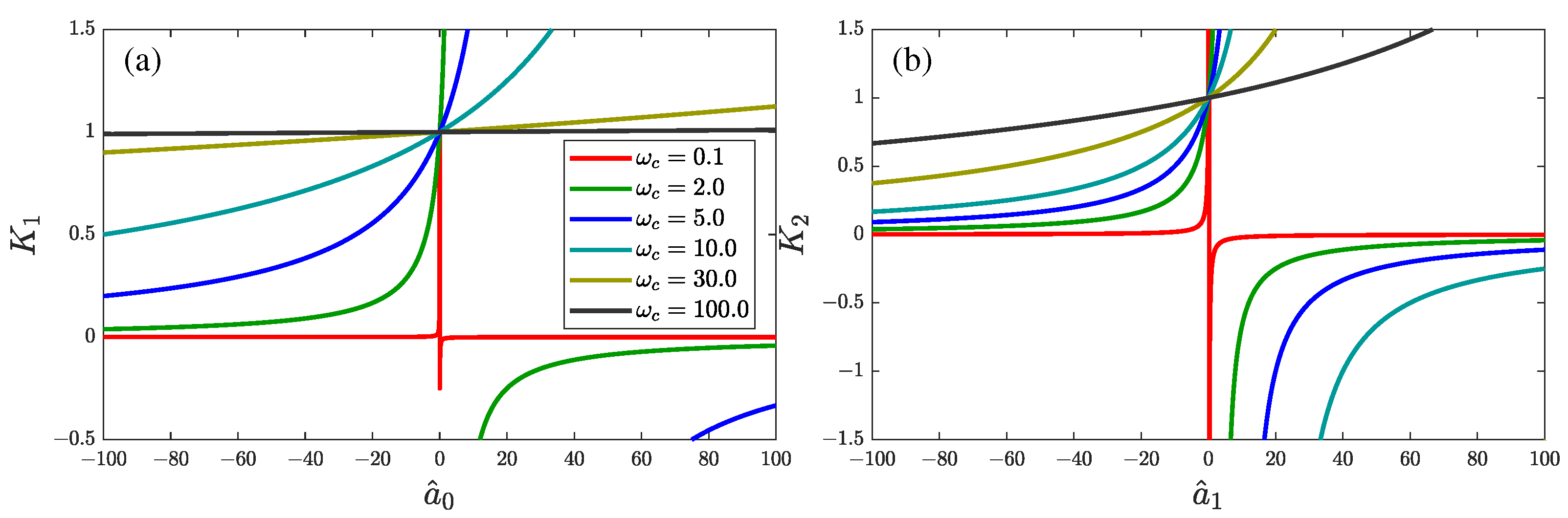
2.2. ADRC Gains Selection

The popular approach to obtaining observer and controller gains is the pole placement method, assuming one multiple pole value, see e.g., [15,39], where one can assume the desired eigenvalues for subsequent system matrices.

The method of selecting parameters assumes that the following functions hold $\mathbf{k}$ and $\mathbf{l}$

$$\det \left(s{\mathbf{I}}_{(n+1)\times (n+1)}-(\mathbf{A}-\mathbf{l}{\mathbf{c}}^{\mathrm{T}})\right)={(s+{\omega }_o)}^{n+1},$$

(11)

$$\det \left(s{\mathbf{I}}_{n\times n}-({\mathbf{A}}_{(1:n)\times (1:n)}-{\mathbf{b}}_{1:n}{\mathbf{k}}^{\mathrm{T}})\right)={(s+{\omega }_c)}^n,$$

(12)

where ${\omega }_c$ is the desired closed-loop bandwidth, ${\omega }_o$ is the observer bandwidth, ${\mathbf{I}}_{n\times n}$ is the identity matrix of dimensions $n\times n$. Depending on the ADRC approach, the matrices and vectors are given by (7).

In general, the gains should be chosen in such a way that the observer works faster than the closed-loop system (faster estimation than the external control loop). According to [36], the relation $5{\omega }_c<{\omega }_o<10{\omega }_c$ should be fulfilled. It should also be noted that increasing the speed of the state observer makes it more sensitive to measurement noise. The influence of the control system parameters on the algorithm operation (for the mfADRC) was analyzed in detail in the paper [40].

There are also alternative methods for fine-tuning the algorithm, such as the linear–quadratic regulator (LQR) [41,42], which minimizes a selected quality index, or a fuzzy approach, where machine intelligence adjusts the system gains [22].

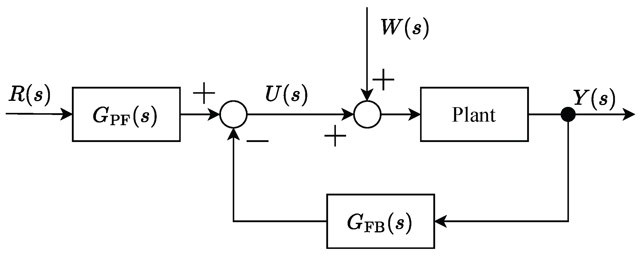
2.3. Control Design for Second-Order System

The study of the influence of model parameters on the gain values and control quality was carried out on a classical second-order model. It can be derived from (2), where $n=2$, ${\mathit{\phi }}^{\mathrm{T}}=[-y,-\dot{y}]$, ${\widehat{\mathit{\theta }}}^{\mathrm{T}}=[{\widehat{a}}_0,{\widehat{a}}_1]$.

Taking into account the input–output dependency, one can obtain a linear part transfer function

$$G\left(s\right){|}_{f=0}={\displaystyle \frac{b}{s^2+a_{1}s+a_0}},$$

(13)

where the real system parameters are considered.

The matrix form of the state–space equations can be obtained for the extended system model (6), where ${\mathbf{x}}^{\mathrm{T}}=[x_1,x_2,x_3]=[y,\dot{y},f(·)]$. The extended state observer is given by the Equation (8), where the matrices are defined as

$$\mathbf{A}=\left[\begin{array}{ccc}0& 1& 0\\ -{\widehat{a}}_0& -{\widehat{a}}_1& 1\\ 0& 0& 0\end{array}\right],\mathbf{b}=\left[\begin{array}{c}0\\ 1\\ 0\end{array}\right],\mathbf{h}=\left[\begin{array}{c}0\\ 0\\ 1\end{array}\right],{\mathbf{c}}^{\mathrm{T}}=\left[\begin{array}{ccc}1& 0& 0\end{array}\right],$$

(14)

and ${\mathbf{l}}^{\mathrm{T}}=[l_1,l_2,l_3]$ is the ESO gains vector.

One can obtain the outer loop control signal (9)

$$u_0=\ddot{r}+{\mathit{\theta }}^{\mathrm{T}}\mathbf{r}+{\mathbf{k}}^{\mathrm{T}}(\mathbf{r}-{\widehat{\mathbf{x}}}_{1:2})=\ddot{r}+({\widehat{a}}_1+k_2)\dot{r}+({\widehat{a}}_0+k_1)r-k_1{\widehat{x}}_1-k_2{\widehat{x}}_2,$$

(15)

and the final control control law (10)

$$u={\displaystyle \frac{1}{\widehat{b}}}\left(\ddot{r}+({\widehat{a}}_1+k_2)\dot{r}+({\widehat{a}}_0+k_1)r-k_1{\widehat{x}}_1-k_2{\widehat{x}}_2-{\widehat{x}}_3\right),$$

(16)

where the reference signal vector takes the form ${\mathbf{r}}^{\mathrm{T}}=[r,\dot{r}]$.

For this configuration, one can obtain ESO and controller gains using the pole-placement method

$$\det \left(s{\mathbf{I}}_{3\times 3}-(\mathbf{A}-\mathbf{l}{\mathbf{c}}^{\mathrm{T}})\right)={(s+{\omega }_o)}^3,$$

(17)

$$\det \left(s{\mathbf{I}}_{2\times 2}-({\mathbf{A}}_{(1:2)\times (1:2)}-{\mathbf{b}}_{1:2}{\mathbf{k}}^{\mathrm{T}})\right)={(s+{\omega }_c)}^2.$$

(18)

Values of the gains are shown below

$$\left\{\begin{array}{ccc}\hfill l_1& =\hfill & 3{\omega }_o-{\widehat{a}}_1\hfill \\ \hfill l_2& =\hfill & 3{\omega }_o^2-({\widehat{a}}_0+l_1{\widehat{a}}_1)\hfill \\ \hfill l_3& =\hfill & {\omega }_o^3\hfill \end{array}\right.,$$

(19)

$$\left\{\begin{array}{ccc}\hfill k_1& =\hfill & {\omega }_c^2-{\widehat{a}}_0\hfill \\ \hfill k_2& =\hfill & 2{\omega }_c-{\widehat{a}}_1\hfill \end{array}\right..$$

(20)

Hence, the parameters also depend on the coefficients of the system. The influence of the values of the model parameters on the change in the gains was investigated for different values of the controller and the ESO bandwidth. For constant bandwidth, there are rational functions

$$L_1={\displaystyle \frac{l_{1,\mathrm{mf}}}{l_{1,\mathrm{mb}}}}={\displaystyle \frac{3{\omega }_o}{3{\omega }_o-{\widehat{a}}_1}}={\displaystyle \frac{1}{1-\frac{{\widehat{a}}_0}{3{\omega }_o}}},$$

(21)

$$L_{2/0}={\left.{\displaystyle \frac{l_{2,\mathrm{mf}}}{l_{2,\mathrm{mb}}}}\right|}_{{\widehat{a}}_1=0}={\displaystyle \frac{3{\omega }_o^2}{3{\omega }_o^2-{\widehat{a}}_0}}={\displaystyle \frac{1}{1-\frac{{\widehat{a}}_0}{3{\omega }_o^2}}},$$

(22)

$$L_{2/1}={\left.{\displaystyle \frac{l_{2,\mathrm{mf}}}{l_{2,\mathrm{mb}}}}\right|}_{{\widehat{a}}_0=0}={\displaystyle \frac{3{\omega }_o^2}{3{\omega }_o^2-(3{\omega }_o-{\widehat{a}}_1){\widehat{a}}_1}}={\displaystyle \frac{1}{1-\frac{(3{\omega }_o-{\widehat{a}}_1){\widehat{a}}_1}{3{\omega }_o^2}}}.$$

(23)

For the controller part, one can obtain dependencies

$$K_1={\displaystyle \frac{k_{1,\mathrm{mf}}}{k_{1,\mathrm{mb}}}}={\displaystyle \frac{{\omega }_c^2}{{\omega }_c^2-{\widehat{a}}_0}}={\displaystyle \frac{1}{1-\frac{{\widehat{a}}_0}{{\omega }_c^2}}},$$

(24)

$$K_2={\displaystyle \frac{k_{2,\mathrm{mf}}}{k_{2,\mathrm{mb}}}}={\displaystyle \frac{2{\omega }_c}{2{\omega }_c-{\widehat{a}}_1}}={\displaystyle \frac{1}{1-\frac{{\widehat{a}}_1}{2{\omega }_c}}}.$$

(25)

As one can see in the Figure 2 and Figure 3, for the unstable system case (when the value of one of the $a_i$ parameters is negative), the higher absolute value of the parameter means a greater change in gains compared to the model-free approach. In the case of a stable object (when all $a_i$ parameters have positive values), the function reaches its maximum point at the point depending on the bandwidth value. The higher the bandwidth value, the steeper the function becomes.

If the parameters of the linear part of the system dynamics are very close to zero $\widehat{\mathit{\theta }}\to \mathbf{0}$, the use of a model-based ADRC will not noticeably affect the gain values, and thus the control quality. With precisely known parameters, only a small improvement in quality can then be seen. It is also worth noting that, for ${\omega }_o\to \infty$ and ${\omega }_o\to \infty$, the obtained gains ratios $L_i$ and $K_i$ are equal to one. Moreover, in the region $L_i>1$, better measurement noise suppression properties of ESO will be obtained in mbADRC (smaller gain values will ensure less noise transfer).

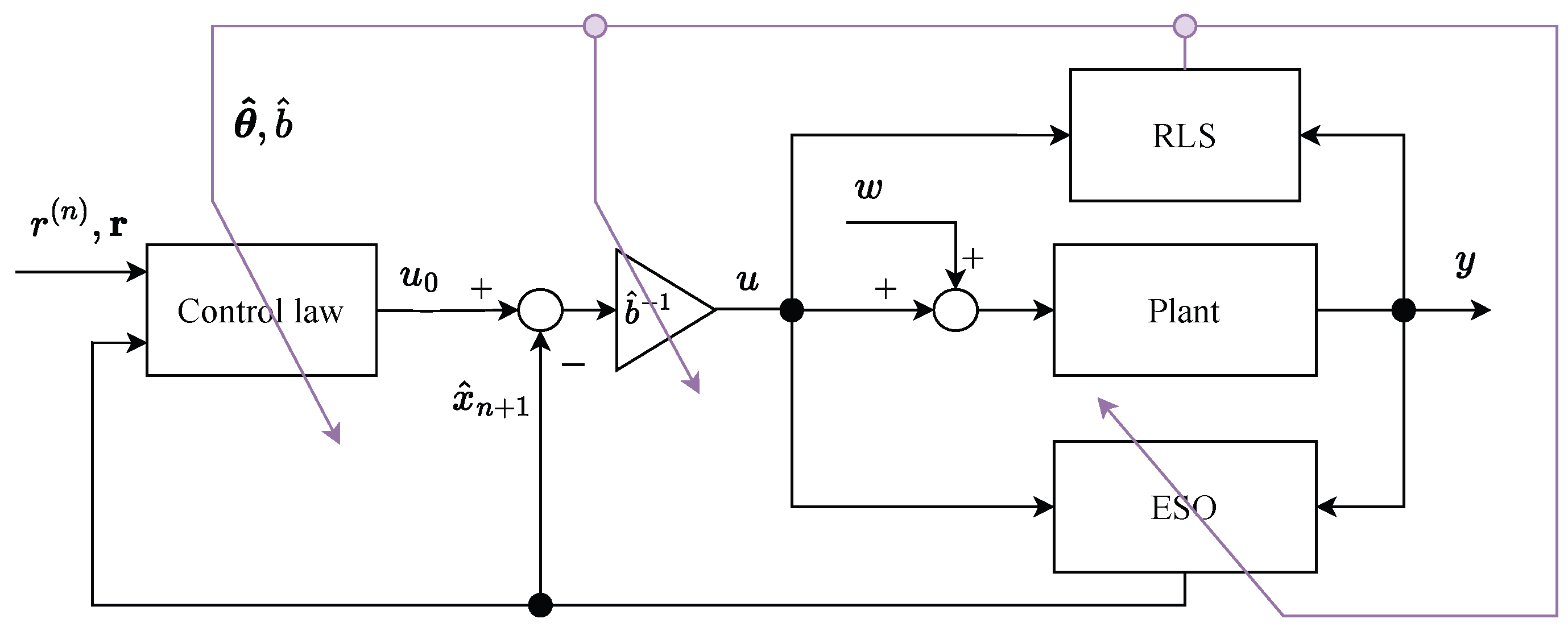
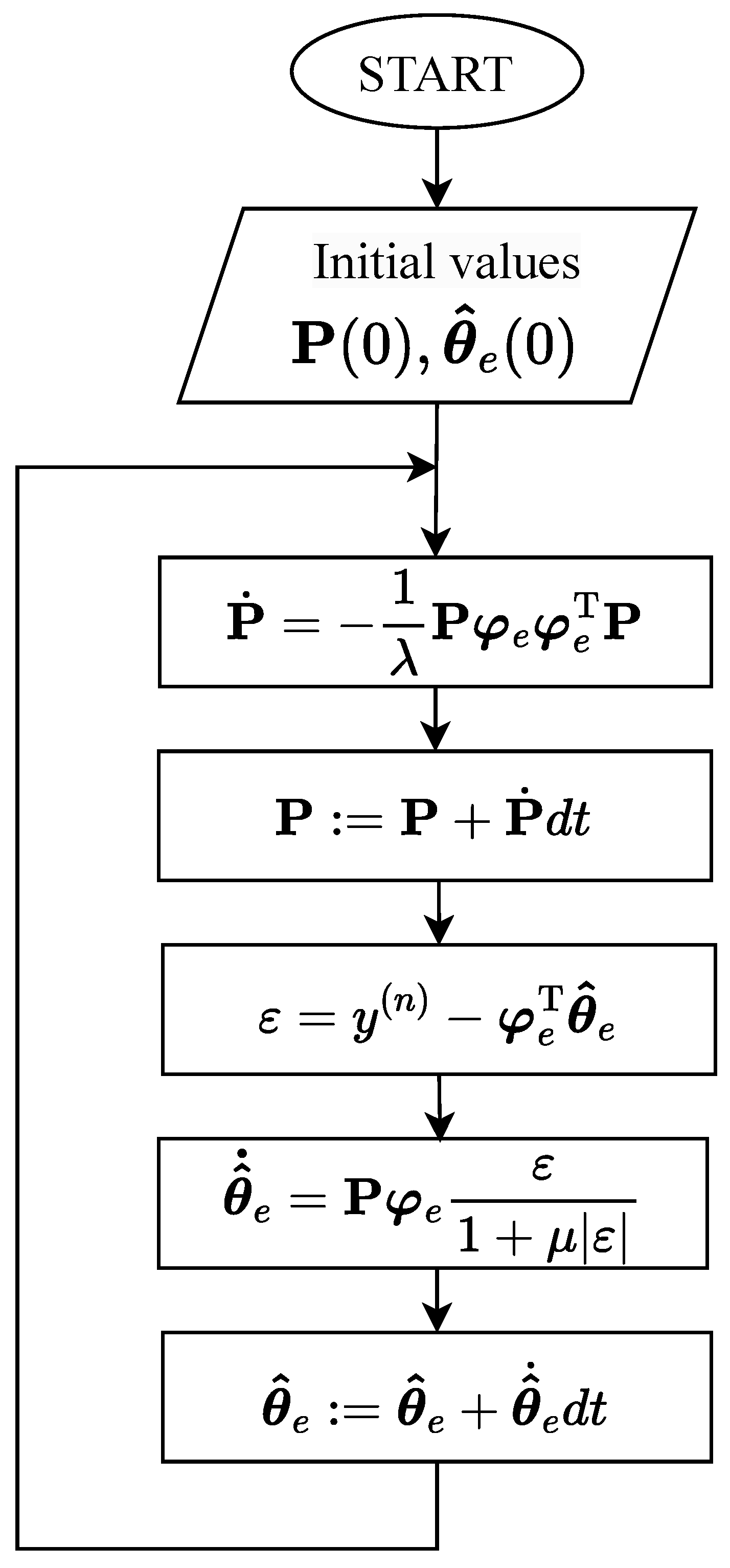
3. Adaptive ADRC Approach

The architecture of the proposed adaptive active disturbance rejection control (adaptADRC) is shown in Figure 4. The proposed adaptADRC is actually also the model-based approach, in which it is generally not required to precisely know the linear part of the system model and input gain. This method updates the model parameters over time, as well as the controller and ESO gains. As a result, even with the lack of knowledge of the physical parameters, the control quality becomes equal to the mbADRC approach. The steady state can be achieved after establishing the parameter estimates.

This approach allows one to fine-tune the ADRC control algorithm during operation without having any initial knowledge of the system parameters. After identification, the operation of the system is very similar to the mbADRC controller. In the case of parametric uncertainties or time-varying parameters, an adaptive approach can noticeably improve the control quality.

The considered system (2) for identification purposes can be rewritten using linear regression form

$$y^{\left(n\right)}={\mathit{\phi }}_e^{\mathrm{T}}{\widehat{\mathit{\theta }}}_e+f(·),$$

(26)

where ${\mathit{\phi }}_e^{\mathrm{T}}={[{\mathit{\phi }}^{\mathrm{T}},u]}^{\mathrm{T}}=[-y,-\dot{y},\dots ,-y^{(n-1)},u]$ is the extended regression vector, ${\widehat{\mathit{\theta }}}_e={[{\mathit{\theta }}^{\mathrm{T}},\widehat{b}]}^{\mathrm{T}}={[{\widehat{a}}_0,{\widehat{a}}_1,\dots ,{\widehat{a}}_{n-1},\widehat{b}]}^{\mathrm{T}}$ is the extended parameters vector (containing the input gain estimate).

The following section presents the algorithm’s protection against outlier disturbances. Furthermore, in the identification literature, it is common to find the inclusion of additional noise in the regression equation, here synonymous with the perturbation function, for example, for an ARMAX-type system [43]. Here, this disturbance analogy can, by the $f(·)$ function, be omitted because parametric identification will be performed only for the linear part.

The recursive least squares method in the continuous time domain [44,45,46] can be described using equations

$$\left\{\begin{array}{c}{\dot{\widehat{\mathit{\theta }}}}_e=\mathbf{P}{\mathit{\phi }}_{e}v\left(\epsilon \right),\hfill \\ \epsilon =y^{\left(n\right)}-{\mathit{\phi }}_e^{\mathrm{T}}{\widehat{\mathit{\theta }}}_e,\hfill \\ \dot{\mathbf{P}}=-{\displaystyle \frac{1}{\lambda }}\mathbf{P}{\mathit{\phi }}_e{\mathit{\phi }}_e^{\mathrm{T}}\mathbf{P},\hfill \end{array}\right.$$

(27)

where $\mathbf{P}$ is the covariance matrix, $\epsilon$ means the identification error, $0<\lambda \le 1$ is the forgetting factor constant.

Instead of the classical linear scaling of the estimation error, one can use a nonlinear function [47]

$$v\left(ϵ\right)={\displaystyle \frac{ϵ}{1+\upsilon ϵ}}$$

(28)

in order to make the algorithm robust to internal or external disturbances occurring in the control process—when, after determining the elements of the covariance matrix, disturbances are strong outliers, and the error increases. The factor $\upsilon$ from the denominator of (28) is generally a design parameter.

Assumption A1.

In this work, identification is performed in a closed control system. To meet the persistent excitation condition of the control signal, it is assumed that the regression vector satisfies for each $t_0>0$

$${\int }_{t_0}^{t_0+t_h}{\mathit{\phi }}_e^{\mathrm{T}}{\mathit{\phi }}_{e}dt\ge c,$$

(29)

where $t_h>0$ and $c>0$. The convergence of parameters is ensured by fulfilling this condition.

In the absence of measurement access to higher derivatives of the output signal, the state variable filters (SVFs) should be used for measurements before processing in the RLS algorithm [48]. The filtered signal derivative is given by,

$$y_F^{\left(i\right)}\left(t\right)={\mathcal{L}}^{-1}\left\{{\displaystyle \frac{s^i}{{(1+s{T}_F)}^n}}Y\left(s\right)\right\},$$

(30)

where $T_F$ is the time constant of the filter. In practice, the $T_F$ value is assumed to be a multiple of sample time of the system, taking care not to filter out useful information about the system (Shannon–Hartley theorem).

In order to better understand the operation of the proposed method, a flowchart for the control system is presented in Figure 5 and for the implementation of the RLS equations in Figure 6.

Stability Analysis of Adaptive ADRC

To facilitate the stability analysis of the proposed modification, the general transfer function of second-order plant (13) is taken into account. Due to the use of a second-order system in experiments, such an example was considered in detailed analyses. However, the closed-loop system structure is presented without losing the generality of the considerations. Assuming that the structure (order of dynamics $n=2$) of (13) is known a priori, but the parameters are uncertain, one can rewrite the model of the system using the linear regression form as in (26)

$$\ddot{y}=\underset{{{\mathit{\phi }}_e}^{\mathrm{T}}}{\underbrace{\left[\begin{array}{ccc}-y& -\dot{y}& u\end{array}\right]}}\underset{{\widehat{\mathit{\theta }}}_e}{\underbrace{\left[\begin{array}{c}{\widehat{a}}_0\\ {\widehat{a}}_1\\ \widehat{b}\end{array}\right]}}.$$

(31)

The employment of the continuous RLS method with the assumed regressor form (31) leads us to the vector of estimated parameters of the model of the system (13) ${\widehat{\mathit{\theta }}}_e={[{\widehat{a}}_0,{\widehat{a}}_1,\widehat{b}]}^{\mathrm{T}}$.

The ADRC controller synthesis is carried out with respect to Section 4, where the estimated system parameters are being updated online. Assuming the constant-value control task, the control law for the outer control loop is obtained as in (16) for $\dot{r}=0$ and $\ddot{r}=0$. Therefore, the final control law takes the form

$$u={\displaystyle \frac{(k_1+{\widehat{a}}_0)r-\left[{\mathbf{k}}^{\mathrm{T}}1\right]\widehat{\mathbf{x}}}{\widehat{b}}},$$

(32)

where ${\mathbf{k}}^{\mathrm{T}}=[k_1,k_2]$ and $\widehat{\mathbf{x}}={[{\widehat{x}}_1,{\widehat{x}}_2,{\widehat{x}}_3]}^{\mathrm{T}}$.

Substitution of the control law (32) into the ESO state Equation (8) leads to the following expression

$$\dot{\widehat{\mathbf{x}}}=\underset{{\mathbf{A}}_{\mathrm{CL}}}{\underbrace{\left(\mathbf{A}-\mathbf{l}{\mathbf{c}}^{\mathrm{T}}-\mathbf{b}\left[{\mathbf{k}}^{\mathrm{T}}1\right]\right)}}\widehat{\mathbf{x}}+(k_1+{\widehat{a}}_0)\mathbf{b}r+\mathbf{l}y,$$

(33)

where $\mathbf{l}={[l_1,l_2,l_3]}^{\mathrm{T}}$. Applying the Laplace transformation on Equation (33) leads to the following expression

$$\widehat{\mathbf{X}}\left(s\right)={(s{\mathbf{I}}_{n+1}-{\mathbf{A}}_{\mathrm{CL}})}^{-1}\left((k_1+{\widehat{a}}_0)\mathbf{b}R\left(s\right)+\mathbf{l}Y\left(s\right)\right),$$

(34)

where the inverse matrix is given as follows

$${(s{\mathbf{I}}_{n+1}-{\mathbf{A}}_{\mathrm{CL}})}^{-1}={\displaystyle \frac{\mathrm{adj}(s{\mathbf{I}}_{n+1}-{\mathbf{A}}_{\mathrm{CL}})}{\det (s{\mathbf{I}}_{n+1}-{\mathbf{A}}_{\mathrm{CL}})}}.$$

(35)

Substituting the transform of the ESO state vector (34) into the transform of the control signal $U\left(s\right)$ from (32) leads to the final form of the control law in the s domain.

$$U\left(s\right)=G_{\mathrm{PF}}\left(s\right)R\left(s\right)-G_{\mathrm{FB}}\left(s\right)Y\left(s\right),$$

(36)

where

$$G_{\mathrm{PF}}\left(s\right)={\displaystyle \frac{(k_1+{\widehat{a}}_0)\left(\det (s{\mathbf{I}}_{n+1}-{\mathbf{A}}_{\mathrm{CL}})-\left[{\mathbf{k}}^{\mathrm{T}}1\right]\mathrm{adj}(s{\mathbf{I}}_{n+1}-{\mathbf{A}}_{\mathrm{CL}})\mathbf{b}\right)}{\widehat{b}\det (s{\mathbf{I}}_{n+1}-{\mathbf{A}}_{\mathrm{CL}})}},$$

(37)

$$G_{\mathrm{FB}}\left(s\right)={\displaystyle \frac{\left[{\mathbf{k}}^{\mathrm{T}}1\right]\mathrm{adj}(s{\mathbf{I}}_{n+1}-{\mathbf{A}}_{\mathrm{CL}})\mathbf{l}}{\widehat{b}\det (s{\mathbf{I}}_{n+1}-{\mathbf{A}}_{\mathrm{CL}})}}.$$

(38)

The prefilter (PF) and feedback (FB) transfer functions defined in (37), (38), can be graphically interpreted with respect to the block diagram presented in Figure 7.

For assumed structure of the plant model (31), transfer functions from (37), (38) takes the following form

$$D_c\left(s\right)=\widehat{b}(s^3+({\widehat{a}}_1+k_2+l_1)s^2+({\widehat{a}}_0+{\widehat{a}}_1{l}_1+k_1+l_2+k_2{l}_1)s),$$

(39)

$$\begin{array}{c}{G}_{\mathrm{PF}}\left(s\right)={\displaystyle \frac{(k_1+{\widehat{a}}_0)s^3+({\widehat{a}}_0{\widehat{a}}_1+{\widehat{a}}_1{k}_1+{\widehat{a}}_0{l}_1+k_1{l}_1)s^2}{D_c\left(s\right)}}+\hfill \\ \hfill +{\displaystyle \frac{({\widehat{a}}_0{k}_1+{\widehat{a}}_0{l}_2+{\widehat{a}}_0^2+{\widehat{a}}_0{\widehat{a}}_1{l}_1+{\widehat{a}}_1{k}_1{l}_1+k_1{l}_2)s+{\widehat{a}}_0{l}_3+k_1{l}_3}{D_c\left(s\right)}},\end{array}$$

(40)

$$G_{\mathrm{PF}}\left(s\right)={\displaystyle \frac{(l_3+k_1{l}_1+k_2{l}_2)s^2+({\widehat{a}}_1{l}_3-{\widehat{a}}_0{k}_2{l}_1+{\widehat{a}}_1{k}_1{l}_1+k_1{l}_2+k_2{l}_3)s+{\widehat{a}}_0{l}_3+k_1{l}_3}{D_c\left(s\right)}},$$

(41)

where observer and controller gains are defined as in (19), (20), respectively.

According to the block diagram of the control loop from Figure 7, and denoting that $G_{\mathrm{PF}}\left(s\right)={\displaystyle \frac{N_{\mathrm{PF}}\left(s\right)}{D_c\left(s\right)}}$, $G_{\mathrm{FB}}\left(s\right)={\displaystyle \frac{N_{\mathrm{FB}}\left(s\right)}{D_c\left(s\right)}}$, it can be derived that the closed-loop transfer function yields

$$G_{\mathrm{CL}}\left(s\right)={\displaystyle \frac{G_{\mathrm{PF}}\left(s\right)G\left(s\right)}{1+G_{\mathrm{FB}}\left(s\right)G\left(s\right)}}={\displaystyle \frac{b{N}_{\mathrm{PF}}\left(s\right)}{(s^2+a_{1}s+a_0)D_c\left(s\right)+b{N}_{\mathrm{FB}}\left(s\right)}},$$

(42)

where $G\left(s\right)$ is the real plant transfer function (13). It should be noted that for current estimates of parameters ${\widehat{\mathit{\theta }}}_e={[{\widehat{a}}_0,{\widehat{a}}_1,\widehat{b}]}^{\mathrm{T}}$, closed-loop is stable since all poles of $G_{\mathrm{CL}}\left(s\right)$ from (42) are located in the left half-plane of the complex variable.

Considering a scenario with a consistent RLS estimator, such that

$$\underset{t\to \infty }{lim}P\left(\right||{\mathit{\theta }}_e-{\widehat{\mathit{\theta }}}_e\left|\right|<\epsilon )=1,$$

(43)

where $\epsilon$ is some positive (small enough) constant, the closed-loop control system (42) takes the following form

$$G_{\mathrm{CL}}\left(s\right)\approx {\displaystyle \frac{{\omega }_c^n{\left(s+{\omega }_o\right)}^{n+1}}{{\left(s+{\omega }_o\right)}^{n+1}{\left(s+{\omega }_c\right)}^n}}={\displaystyle \frac{{\omega }_c^n}{{(s+{\omega }_c)}^n}}.$$

(44)

The above expression is the desired transfer function for the closed-loop control system.

Remark 3.

Assuming the trajectory tracking task, the control law (32) takes the following form

$$u={\displaystyle \frac{{(\mathbf{k}+\widehat{\mathit{\theta }})}^{\mathrm{T}}\mathbf{r}+r^{\left(n\right)}-\left[{\mathbf{k}}^{\mathrm{T}}1\right]\widehat{\mathbf{x}}}{\widehat{b}}},$$

(45)

and, if (43) is satisfied, the closed-loop system form of (42) is shown below

$$G_{\mathrm{CL}}\left(s\right)\approx {\displaystyle \frac{{(s+{\omega }_c)}^n{\left(s+{\omega }_o\right)}^{n+1}}{{\left(s+{\omega }_o\right)}^{n+1}{\left(s+{\omega }_c\right)}^n}}=1.$$

(46)

However, parameterization of the algorithm must ensure the stability of the control system without the feedforward part.

4. Results of the Experiments and Simulations

Experiments were carried out to check the control quality for both ADRC approaches considered depending on the bandwidth values and the model parameters in the linear case and with the nonlinear part considered as part of the system disturbance. In the last part of the section, the possibility of identifying parameters during the operation of the system was examined, using the recursive least squares method, as shown in Figure 4. The real plant, a DC motor, was used for the experiments.

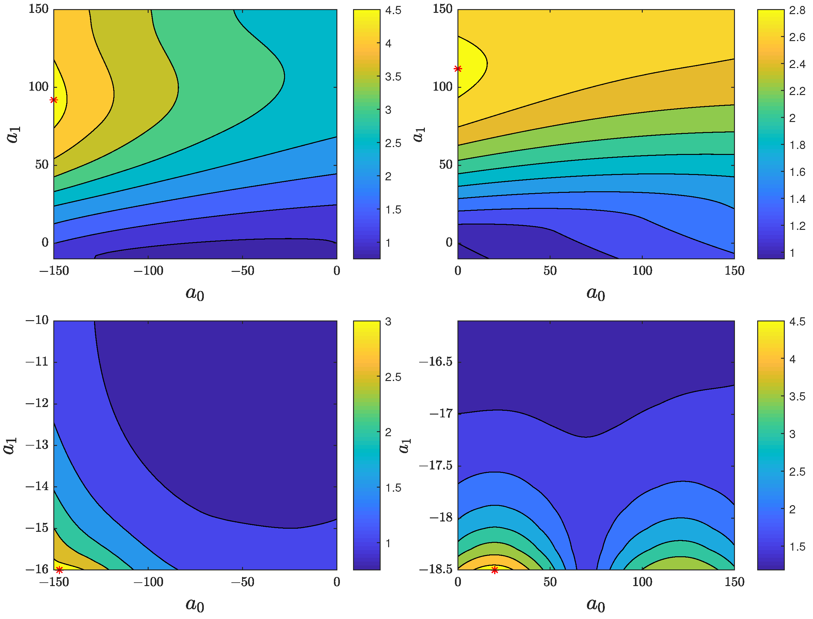
4.1. Influence of System Parameters on the Control Quality

The influence of the second-order system parameters (13) on the control quality with a constant reference value and external disturbance signal was examined. The integral of absolute error (IAE) quality index was used

$$\mathrm{IAE}={\int }_0^{t_h}|r-y|dt,$$

(47)

where $t_h$ is the simulation horizon. To compare mf- and mbADRC, the ratio of indices ${\displaystyle \frac{{\mathrm{IAE}}_{\mathrm{mf}}}{{\mathrm{IAE}}_{\mathrm{mb}}}}$ was determined for each pair of parameters $(a_0,a_1)$, assuming constant-bandwidth ${\omega }_c$, ${\omega }_o$ values for each experiment. As this ratio increases, an increasing advantage of the approach based on the linear part of the model is observed. The tests were carried out for $r=2$ and $t_h=4$ s and in the presence of external disturbance $w\left(t\right)=5·1(t-2)$. In Figure 8 and Figure 9, one can see the quality index IAE ratio for various system parameters. This way, it is possible to assess the influence of the parameters on the control process. The points where the ratio of indices reached the highest value (the local maxima) are marked in red. In this presentation form, a higher value of the index ratio means a greater advantage of mbADRC over mfADRC (when IAE_mb in the denominator is smaller than IAE_mf in the numerator).

The tests were performed in the area where the mfADRC system was stable. Additionally, a precise knowledge of the system parameters was assumed, so ${\widehat{a}}_i=a_i$. According to Figure 8, the area for $a_0<0$ or $a_1<0$, the influence of unstable plant dynamics (for a higher modulus of $a_i$) cannot be successfully rejected by the mfADRC algorithm, and this implies the need to increase the observer bandwidth to provide stability of the system. Increasing ${\omega }_o$ implies a better ability to estimate the total disturbance, but the closed-loop system becomes sensitive to measurement noise. The limit of absolute values of the parameters $a_0$ and $a_1$ was set to 150 because, in practice, there is rarely a control system with a dominant time constant with such a low value. There is also a visible tendency when increasing parameters. In the bottom right part of the figure (positive $a_0$ and negative $a_1$ values), the start of the range for the parameter $a_1$ was selected for $-16$ due to the noticeable differences in the IAE factor for smaller parameters, which causes deterioration of the plot resolution.

The results of the conducted simulations show that the advantage of the mbADRC approach is greater for parameters with a higher modulus, where information about the dynamics of the system positively affects stability and control quality. The local maxima of the computing ratio in the plane with $-a_0,+a_1$; $-a_0,-a_1$; and $+a_0,-a_1$ are close to an unstable control loop with mfADRC, and it is necessary to increase the ESO bandwidth to ensure stable system operation. It also means that, in general, the mbADRC requires less bandwidth than the mfADRC approach, which is also a positive factor in a real system with measurement noise. The positive impact on stability cannot be confirmed in the plane with positive $a_0$ and $a_1$, where the plant and closed-loop system are asymptotically stable, and for limited external disturbance, the closed loop will be stable for any parameters. However, one can still notice that the advantages of control quality with the mbADRC approach are increasing together with the $a_1$ parameter of the system. It is stable but difficult to control due to the high unmodeled velocity part; the dynamics of the plant (values: close to 0 and $-150$) cannot be successfully controlled by mfADRC for any observer and controller bandwidth. However, including information on these dynamics into the mbADRC approach noticeably increases control quality. As one can see in Figure 2 and Figure 3, this is the area where the relative observer and controller gains values show the greatest differences between the gains in both ADRC approaches.

Then, simulations with a substantially higher ESO bandwidth value (${\omega }_o=500$) were conducted. Based on Figure 9, only slight differences between the considered approaches can be deduced. The high observer bandwidth ensures a very fast estimation of the total disturbance even in the mfADRC approach for high parameter modulus values. For this reason, the ratio of quality indices in the entire graph area is very close to one. However, in practice, this approach causes a very high sensitivity to measurement noise.

In general, a positive impact can be observed by including a system model, especially for higher absolute values of the object parameters, because of the greater impact on the dynamics of the plant (harder to control with the mfADRC variant without observer and controller tuning) and mbADRC gain values (19)–(20). For the absolute value of the parameters close to zero, the performance of mbADRC is reduced to mfADRC or even the same, which can be seen in areas where the ratio of the coefficients is close to unity.

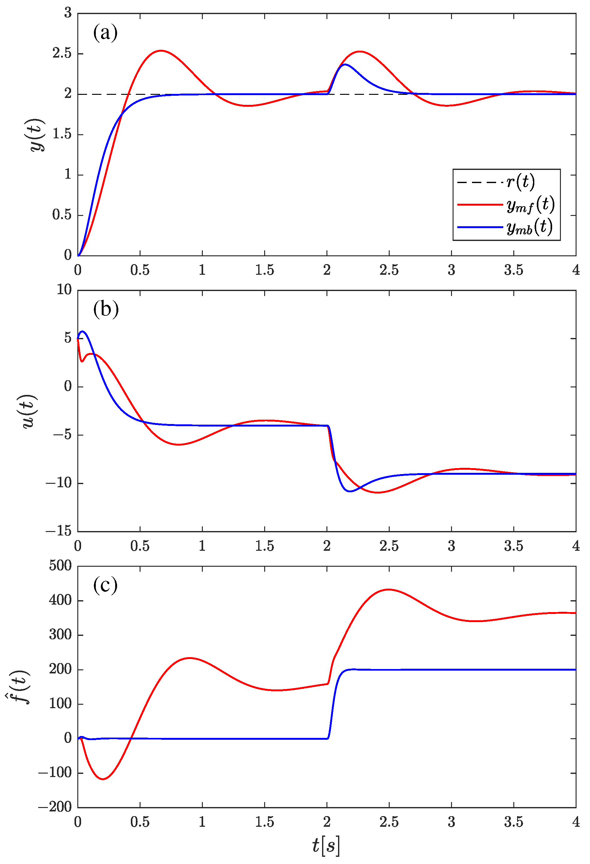
4.2. Simulation Plant–Control System Analysis for mfADRC and mbADRC

As has been shown, with an increase in the absolute value of the parameters, the influence of the model part on the reinforcement and operation of the system increases. A linear simulational system, as in [27], was selected in which parameter values allow for demonstrating the differences between the presented approaches. Below, one can see a comparison of mf- and mbADRC, for the system (named generic plant) given by the differential equation and transfer function

$$\ddot{y}=80y-30\dot{y}+40u+w,$$

$$G_p\left(s\right){|}_{w=0}={\displaystyle \frac{40}{s^2+30s-80}},$$

where the external disturbance is given as $w\left(t\right)=5·1(t-2)$. The assumed parameters of the control algorithms were ${\omega }_c=10$, ${\omega }_o=50$, $\widehat{b}=40$. For all cases, the value of the parameter $\widehat{b}$ was assumed to be as close as possible to the real one. The selected bandwidth of the closed-loop system ${\omega }_c$ was selected to provide the desired sensitivity of the controller. On the other hand, for the observer, the bandwidth ${\omega }_o$ value was selected with respect to the separation principle [36]. The simulation results are shown in Figure 10.

In the above case, mfADRC was unable to ensure the desired response nature due to the accumulation of total disturbance from the unconsidered part of the model dynamics. As a result, the response was slower than expected, resulting in overshoot and oscillations. For this case, the quality index ratio ${\displaystyle \frac{{\mathrm{IAE}}_{\mathrm{mf}}}{{\mathrm{IAE}}_{\mathrm{mb}}}}$ is equal to ${\displaystyle \frac{1.0366}{0.4987}}=2.0786$.

If the real parameters of the object are known, the total disturbance function tends to zero in the initial part of the simulation and then estimates the object’s response to the disturbance signal given in the middle time of the simulation.

Based on the simulation, it is visible that, in some cases, it is not possible to obtain the desired control quality for the selected algorithm gains without including information about the model in the system synthesis process. Estimates of the total disturbance function may cause oscillations in the control signal as well as in the system output.

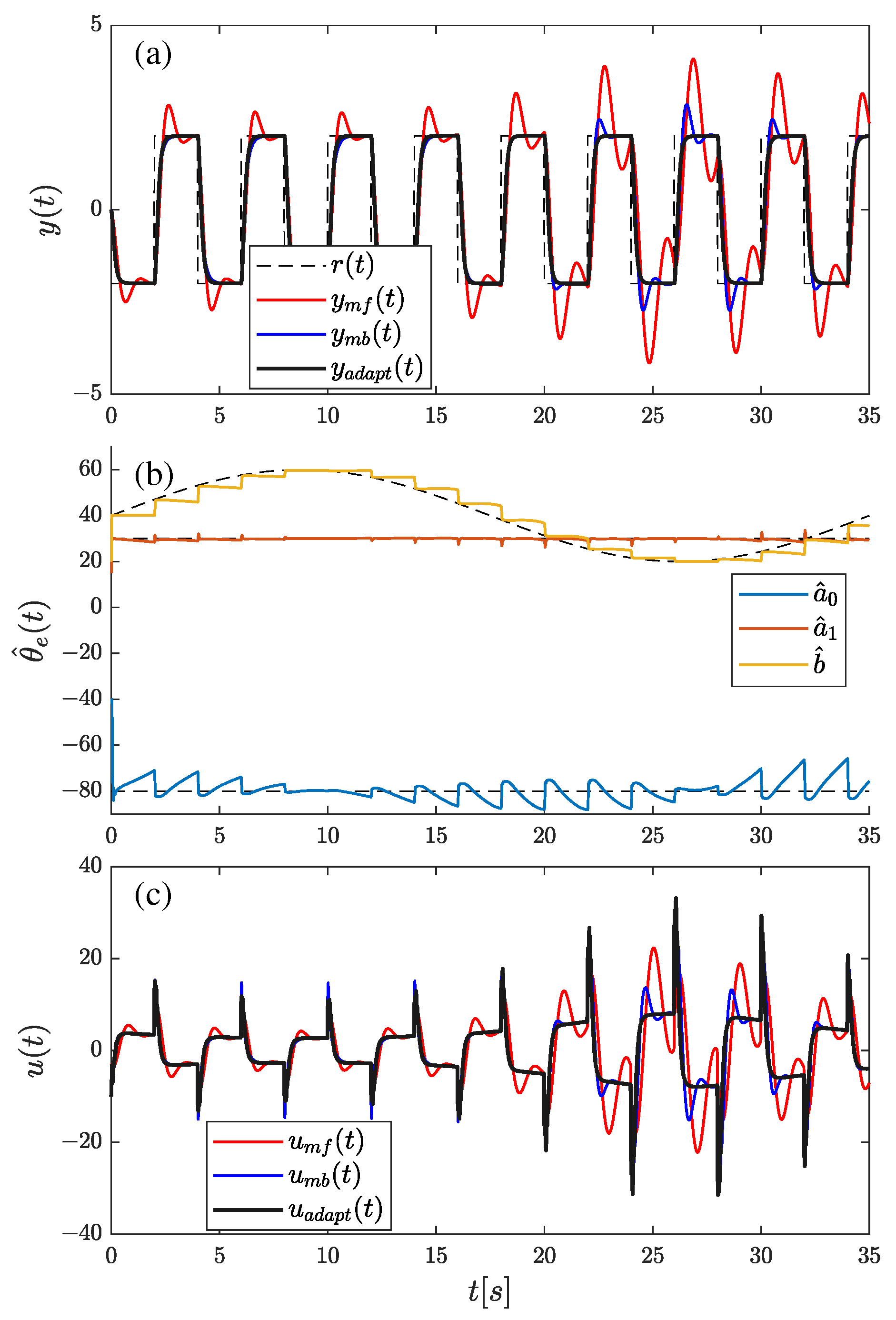
4.3. Simulation Plant–Control Plant with Time-Varying Parameter

The object given by equation

$$\ddot{y}=-a_{0}y-a_1\dot{y}+\underset{b\left(t\right)}{\underbrace{\left(A_0+Asin(2\pi /35·t)\right)}}u+w,$$

where the parameter values $a_0=-80$, $a_1=30$, $A_0=40$, $A=20$ are considered. The rectangular reference signal was assumed $r\left(t\right)=2\mathrm{Rect}\left(2\pi {\displaystyle \frac{1}{4}}t\right)$. The mfADRC and mbADRC approaches were compared with the proposed adaptive approach. The assumed parameters of the control algorithms were ${\omega }_c=10$, ${\omega }_o=50$. For the model-free and model-based methods $\widehat{b}=A_0=40$, for mbADRC, additionally $a_0=-80$, $a_1=30$ were assumed. In the adaptive approach, initial conditions $\widehat{\mathit{\theta }}\left(0\right)=0.5{[-80,30,40]}^{\mathrm{T}}$ were assumed. The model parameters were updated at each time step, and the assumed forgetting coefficient was $\lambda =0.97$. The simulation results are shown in Figure 11.

For the mfADRC approach, overshoots appear throughout the experiment, which can be eliminated by underestimating the input gain value [49] (the first half of the simulation time, when $\widehat{b}\left(t\right)<b\left(t\right)$). In the mbADRC, a deterioration in control quality (occurrence of overshoots) can be observed in the second part of the experiment. Overshoots occur when $\widehat{b}\left(t\right)$ is overestimated, and in the case of half-period (underestimated) there is no deterioration because, in general, underestimation improves stability, as mentioned above. Assuming a constant value of this parameter in the control algorithm is insufficient in this case because the properties of the control system change depending on the work point.

The use of the adaptive approach allowed us to achieve the desired control quality in the full scope of the experiment. The correct estimation of the parameters and adjustment to the input gain value of the variable are observed. Improving the operation of the system in the adaptive approach resulted in larger values of the control signal at the moment of switching the reference value. However, this action allowed the overshoots to be completely eliminated.

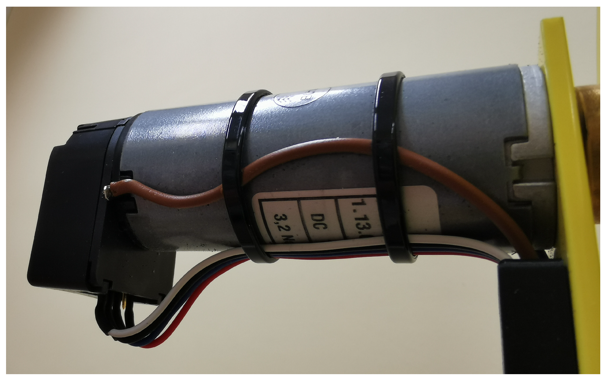
4.4. Real Plant–DC Motor

For the next experiments, a real object was used—a direct current (DC) motor, where the input signal is the voltage (values in the range $[-12,12]$ V), and the output signal is the motor velocity [15]

$${\displaystyle \frac{d^{2}y\left(t\right)}{d{t}^2}}=-{\displaystyle \frac{RJ+Lc}{LJ}}{\displaystyle \frac{dy\left(t\right)}{dt}}-{\displaystyle \frac{Rc+{\left(k_{\varphi }\right)}^2}{LJ}}y\left(t\right)+{\displaystyle \frac{k_{\varphi }}{LJ}}u\left(t\right)+w\left(t\right),$$

(48)

where y [rad/s] is the measured angular velocity, $R=2.4$ Ω is the armature resistance, $L=0.11$ H is the armature inductance, $J=2.3\times {10}^{-4}$ kg·m² is the shaft inertia, $c=8.82\times {10}^{-5}$ Nm/rad is the damping coefficient, $k_{\varphi }=0.016$ Vs/rad is the torque constant. The system parameters are shown in

Table 1. Parameters of the DC motor used in the experiments.

Symbol	Unit	Value	Name
R	Ω	$2.4$	armature resistance
L	H	$0.11$	armature inductance
J	kg·m2	$2.3\times {10}^{-4}$	shaft inertia
c	Nm/rad	$8.82\times {10}^{-5}$	damping coefficient
$k_{\varphi }$	Vs/rad	$0.016$	torque constant

. The photo of the used DC motor test bench is in Figure 12.

The system can be described by the second-order transfer function (13). Based on the physical parameters of the system, the nominal model parameters were obtained: $a_0={\displaystyle \frac{Rc+{\left(k_{\varphi }\right)}^2}{LJ}}=18$, $a_1={\displaystyle \frac{RJ+Lc}{LJ}}=22$, $b={\displaystyle \frac{k_{\varphi }}{LJ}}=780$. It determines the extended parameter vector of the system ${\mathit{\theta }}_e={[18,22,780]}^{\mathrm{T}}$.

The experiments on the DC motor were carried out for two control task scenarios:

• Constant-value control, for which the reference velocity yields

  $$r\left(t\right)=\mathrm{Rect}\left(2\pi {\displaystyle \frac{1}{20}}t\right),$$
• Trajectory tracking control, for which the reference velocity yields

  $$r\left(t\right)=sin\left(2\pi {\displaystyle \frac{1}{10}}t\right).$$

Three variants of ADRC during the experiments were considered: mfADRC, for which ${\widehat{a}}_i=0$ and $\widehat{b}=b$, thus ${\widehat{\mathit{\theta }}}_e=[0,0,780]$; mbADRC, for which ${\widehat{\mathit{\theta }}}_e={\mathit{\theta }}_e$ and our proposition, the adaptive ADRC with on-line parameter identification (adaptADRC). The initial value of the extended vector of estimated parameters ${\widehat{\mathit{\theta }}}_e\left(0\right)=0.5{\mathit{\theta }}_e$ was assumed.

The controller and observer bandwidth values (ADRC design parameters) were selected as ${\omega }_c=3.4$, ${\omega }_o=40$. For both scenarios of the control task, external disturbances were assumed as $w\left(t\right)=4·1(t-5)+4·1(t-15)$. Furthermore, the summary of parameter selection for the compared ADRC approaches can be found in

Table 2. Summary of parameter selection for the compared ADRC approaches.

Approach	Parameter
	$\mathit{n}$	${\widehat{\mathit{a}}}_{\mathit{i}}$	$\widehat{\mathit{b}}$	$\mathbf{l}$	$\mathbf{k}$
mfADRC	const	0	const	const	const
mbADRC	const	const	const	const	const
adaptADRC (our)	const	var *	var *	var	var

*—initial values required.

.

For quantitative analysis of the experimental results, three quality indices were obtained, where the first one was the IAE index defined in (47), the second one yields

$$J_u={\int }_0^{t_h}{u}^2\left(t\right)dt,$$

(49)

which represents the control signal energy, and the last one yields

$$J_{\mathrm{fit}}={\int }_0^{t_h}\left|y_{\mathrm{ref}}-y\right|dt,$$

(50)

which represents the absolute value from the difference between the desired dynamics $y_{\mathrm{ref}}$ and the system output y. The reference dynamics are considered as

$$y_{\mathrm{ref}}\left(t\right)={\mathcal{L}}^{-1}\left\{G_{\mathrm{CL}}\left(s\right)R\left(s\right)\right\},$$

(51)

where $R\left(s\right)$ is the Laplace transform of the reference signal, $G_{\mathrm{CL}}\left(s\right)$ takes the form (44) in the case of constant-value control task, and (46) for trajectory tracking control task.

Furthermore, the three indices (47), (49), (50) were also calculated for the second part of the experiment, where the steady state of the parameters estimated by RLS was reached: $\mathrm{IAE}={\int }_{t_h/2}^{t_h}\left|e\left(t\right)\right|dt$, $J_u={\int }_{t_h/2}^{t_h}{u}^2\left(t\right)dt$, $J_{\mathrm{fit}}={\int }_{t_h/2}^{t_h}\left|y_{\mathrm{ref}}-y\right|dt$.

A comparison of the experimental results was made using the time responses for mf-, mb-, and adaptADRC, shown in Figure 13 and Figure 14, and the the quality indices for the performed experiments can be seen in

Table 3. Quality index values for conducted experiments for the whole time and for the second half-time. The lowest index values are marked in bold.

Approach	IAE	${\mathit{J}}_{\mathbf{fit}}$	${\mathit{J}}_{\mathit{u}}$	IAE	${\mathit{J}}_{\mathbf{fit}}$	${\mathit{J}}_{\mathit{u}}$
	The Whole Experiment			After Adaptation Process
Rectangular reference signal
mfADRC	291.2230	116.0525	874.1242	185.0328	67.8664	821.9041
mbADRC	207.7081	35.3479	893.9396	132.7821	17.9658	839.0451
adaptADRC (our)	282.869	111.1597	932.4270	130.0112	16.8768	837.1188
Sinusoidal reference signal
mfADRC	210.9012	210.9012	729.0449	102.5087	102.5087	521.9984
mbADRC	43.4767	43.4767	724.9985	19.1165	19.1165	519.6592
adaptADRC (our)	60.2311	60.2311	788.1805	13.4748	13.4748	520.1384

.

Based on the obtained results, generally it can be concluded that the use of mbADRC can improve control quality compared to the mfADRC approach. According to results from the experiment in the constant-value control regime (Figure 14), in mfADRC’s closed-loop performance, there is an overshoot. It is caused by values of the plant parameters ${\mathit{\theta }}^{\mathrm{T}}=[18,22]$ (see Figure 8). Both model-based approaches (mbADRC and adaptADRC after the adaptation process) almost provided a nominal closed-loop performance (based on the $J_{\mathrm{fit}}$ index from Table 3) control quality due to better compensation of the linear part of system dynamics. In the experiment where the trajectory tracking control task was considered (Figure 13), despite incorporating the feedforward part in the control law, with the mfADRC approach, the range of modeling uncertainty was disallowed to track the sinusoidal reference signal with assumed frequency. In that case, both model-based approaches made it possible to realize the control task accurately.

It is worth noting that the resultant closed-control loop performance in steady-state adaptADRC is pretty close to the desired (reference) dynamics defined in (44), (46), which confirms the stability analysis conducted in Section 3. Moreover, adaptADRC, despite the lack of required a priori knowledge about the model of the system, allows for tracking the reference trajectory with nominal quality, which is provided by the mbADRC approach (which requires accurate knowledge about the model of the system).

In the case of adaptADRC, an increase in the control cost can be observed, which is caused by the operation of the system in the initial phase of the experiment, before the parameter values become established. The initial poorer control quality during parameter setting is visible, but after the adaptation process, the robustness to external disturbance was also maintained.

In some cases, mfADRC can even destabilize the closed-loop operation, while the mbADRC approach in each of the tested cases allowed us to maintain stability and follow the given dynamics of the closed-loop system. For the initial parameters equal to ${\widehat{\mathit{\theta }}}_e\left(0\right)=0.5{\mathit{\theta }}_e$, the algorithm ensures fast establishment of the parameters estimates. The negative impact of the uncertainty of the parameters on the graphs is imperceptible.

5. Discussion and Conclusions

The article analyzes the differences between the three structures of the ADRC algorithm for different control plant cases and configurations. The basic model-free version of ADRC generally allows rejection of disturbances; however, for a certain range of tested parameter values, control quality deterioration or even destabilization of a closed-loop system may occur despite the tuning of such an algorithm. In the case of model-based ADRC, the state matrix includes the known dynamics of the linear part of the object, which also affects the values of the algorithm gains. Thanks to this combination of classical state feedback with active disturbance compensation, it is possible to improve the robustness of the system and increase the range of acceptable amplification for a given object structure. The parameter range for the linear system has been extended with respect to the mbADRC paper in which this approach was proposed [27]. Moreover, reducing the ESO gain values in mbADRC can result in better suppression of measurement noise in comparison to approaches involving regression outside the matrices [33].

The combination of model-based ADRC with the recursive least-squares method of parameter identification was proposed and analyzed. The stability analysis for the proposed adaptive ADRC structure was also performed. The experiments conducted on real plant (DC motor) confirm the theoretical considerations. If the persistent excitation in the closed-loop system is met, the RLS estimator becomes convergent. This allows us to reach the desired closed-loop performance, even in the case of a trajectory tracking control task, without the need to know the model parameters a priori. In the mbADRC approach, it can be reached only when the parameters are precisely known.

Parameter identification also allows one to detect changes resulting from wear or failure of components, which could result in a deterioration in the control quality or even destabilization of the system for a fixed-gains approaches. In the case of variable system parameters, the proposed adaptADRC approach allows us to achieve better closed-loop performance even than the mbADRC. The online parametric identification ensures the flexibility of the model used in the controller synthesis, whereas, in fixed-gains algorithms, it is assumed that the parameters of the system are time-invariant. The use of the presented adaptive approach is a way to solve the parametric uncertainty problem discussed in the papers [38,50].

In the future, it is planned to extend the research to check the impact of a larger non-linear class on the robustness of the system with different variants of including the model in the algorithm. The possibility of improving control quality by changing the state estimation method, for example, by using Kalman filtering instead of ESO, will also be checked. The operation of other plants with proposed ADRC modifications will also be examined.

References

1. Aoudni, Y.; Kalra, A.; Azhagumurugan, R.; Ahmed, M.A.; Wanjari, A.K.; Singh, B.; Bhardwaj, A. Metaheuristics based tuning of robust PID controllers for controlling voltage and current on photonics and optics. Opt. Quantum Electron. 2022, 54, 809. [Google Scholar] [CrossRef]
2. Feng, X.; Li, X.; Li, S.; Pan, F. Secure state estimation for unmanned aircraft cyber-physical systems under multiple attacks. Asian J. Control 2022, 24, 818–833. [Google Scholar] [CrossRef]
3. Gao, Z. Active disturbance rejection control: A paradigm shift in feedback control system design. In Proceedings of the 2006 American Control Conference, Minneapolis, MI, USA, 14–16 June 2006; pp. 2399–2405. [Google Scholar] [CrossRef]
4. Guo, B.; Bacha, S.; Alamir, M. A review on ADRC based PMSM control designs. In Proceedings of the IECON 2017-43rd Annual Conference of the IEEE Industrial Electronics Society, Beijing, China, 29 October–1 November 2017; pp. 1747–1753. [Google Scholar] [CrossRef]
5. Yang, X.; Huang, Q.; Jing, S.; Zhang, M.; Zuo, Z.; Wang, S. Servo system control of satcom on the move based on improved ADRC controller. Energy Rep. 2022, 8, 1062–1070. [Google Scholar] [CrossRef]
6. Fang, Q.; Zhou, Y.; Ma, S.; Zhang, C.; Wang, Y.; Huangfu, H. Electromechanical Actuator Servo Control Technology Based on Active Disturbance Rejection Control. Electronics 2023, 12, 1934. [Google Scholar] [CrossRef]
7. Bai, K.; Luo, Y.; Dan, Z.; Zhang, S.; Wang, M.; Qian, Q.; Zhong, J. Extended State Observer based Attitude Control of a Bird-like Flapping-wing Flying Robot. J. Bionic Eng. 2020, 17, 708–717. [Google Scholar] [CrossRef]
8. Tan, L.; Liang, S.; Su, H.; Qin, Z.; Li, L.; Huo, J. Research on Amphibious Multi-Rotor UAV Out-of-Water Control Based on ADRC. Appl. Sci. 2023, 13, 4900. [Google Scholar] [CrossRef]
9. Chang, S.; Wang, Y.; Zuo, Z.; Zhang, Z.; Yang, H. On fast finite-time extended state observer and its application to wheeled mobile robots. Nonlinear Dyn. 2022, 110, 1473–1485. [Google Scholar] [CrossRef]
10. Hai, X.; Wang, Z.; Feng, Q.; Ren, Y.; Xu, B.; Cui, J.; Duan, H. Mobile robot ADRC with an automatic parameter tuning mechanism via modified pigeon-inspired optimization. IEEE/ASME Trans. Mechatron. 2019, 24, 2616–2626. [Google Scholar] [CrossRef]
11. Gao, J.; Liang, X.; Chen, Y.; Zhang, L.; Jia, S. Hierarchical image-based visual serving of underwater vehicle manipulator systems based on model predictive control and active disturbance rejection control. Ocean Eng. 2021, 229, 108814. [Google Scholar] [CrossRef]
12. Chen, C.F.; Du, Z.J.; He, L.; Wang, J.Q.; Wu, D.M.; Dong, W. Active disturbance rejection with fast terminal sliding mode control for a lower limb exoskeleton in swing phase. IEEE Access 2019, 7, 72343–72357. [Google Scholar] [CrossRef]
13. Dao, Q.T.; Dinh, V.V.; Trinh, M.C.; Tran, V.C.; Nguyen, V.L.; Duong, M.D.; Bui, N.T. Nonlinear Extended Observer-Based ADRC for a Lower-Limb PAM-Based Exoskeleton. Actuators 2022, 11, 369. [Google Scholar] [CrossRef]
14. Michalski, J.; Retinger, M.; Kozierski, P.; Giernacki, W. Position Control of Crazyflie 2.1 Quadrotor UAV Based on Active Disturbance Rejection Control. In Proceedings of the 2023 International Conference on Unmanned Aircraft Systems (ICUAS), Warsaw, Poland, 6–9 June 2023; pp. 1106–1113. [Google Scholar] [CrossRef]
15. Lakomy, K.; Giernacki, W.; Michalski, J.; Madonski, R. Active Disturbance Rejection Control (ADRC) Toolbox for MATLAB/Simulink. arXiv 2021, arXiv:2112.01614. [Google Scholar]
16. Madonski, R.; Shao, S.; Zhang, H.; Gao, Z.; Yang, J.; Li, S. General error-based active disturbance rejection control for swift industrial implementations. Control Eng. Pract. 2019, 84, 218–229. [Google Scholar] [CrossRef]
17. Madonski, R.; Herbst, G.; Stankovic, M. ADRC in output and error form: Connection, equivalence, performance. Control Theory Technol. 2023, 21, 56–71. [Google Scholar] [CrossRef]
18. Herbst, G. Transfer function analysis and implementation of active disturbance rejection control. Control Theory Technol. 2021, 19, 19–34. [Google Scholar] [CrossRef]
19. Herbst, G.; Madonski, R. Tuning and implementation variants of discrete-time ADRC. Control Theory Technol. 2023, 21, 72–88. [Google Scholar] [CrossRef]
20. Miklosovic, R.; Radke, A.; Gao, Z. Discrete implementation and generalization of the extended state observer. In Proceedings of the 2006 American Control Conference, Minneapolis, MI, USA, 14–16 June 2006; pp. 2209–2214. [Google Scholar] [CrossRef]
21. Carvajal, B.V.M.; Sáez, J.S.; Rodríguez, S.G.N.; Iranzo, M.M. Modified Active Disturbance Rejection Predictive Control: A fixed-order state–space formulation for SISO systems. ISA Trans. 2023, 142, 148–163. [Google Scholar] [CrossRef]
22. Zhang, Z.; Yang, Z.; Zhou, G.; Liu, S.; Zhou, D.; Chen, S.; Zhang, X. Adaptive fuzzy active-disturbance rejection control-based reconfiguration controller design for aircraft anti-skid braking system. Actuators 2021, 10, 201. [Google Scholar] [CrossRef]
23. Lv, C.; Wang, B.; Chen, J.; Zhang, R.; Dong, H.; Wan, S. Research on a Torque Ripple Suppression Method of Fuzzy Active Disturbance Rejection Control for a Permanent Magnet Synchronous Motor. Electronics 2024, 13, 1280. [Google Scholar] [CrossRef]
24. Kicki, P.; Łakomy, K.; Lee, K.M.B. Tuning of extended state observer with neural network-based control performance assessment. Eur. J. Control 2022, 64, 100609. [Google Scholar] [CrossRef]
25. Bai, C.; Zhang, Z. A least mean square based active disturbance rejection control for an inertially stabilized platform. Optik 2018, 174, 609–622. [Google Scholar] [CrossRef]
26. Zhang, Z.; Cheng, J.; Guo, Y. PD-based optimal ADRC with improved linear extended state observer. Entropy 2021, 23, 888. [Google Scholar] [CrossRef]
27. Zhou, R.; Tan, W. A generalized active disturbance rejection control approach for linear systems. In Proceedings of the 2015 IEEE 10th Conference on Industrial Electronics and Applications (ICIEA), Auckland, New Zealand, 15–17 June 2015; pp. 248–255. [Google Scholar] [CrossRef]
28. Fu, C.; Tan, W. Tuning of linear ADRC with known plant information. ISA Trans. 2016, 65, 384–393. [Google Scholar] [CrossRef]
29. Hao, S.; Liu, T.; Geng, X.; Wang, Y. Anti-windup ADRC design for temperature control systems with output delay against asymmetric input constraint. ISA Trans. 2023, 2023, 519–530. [Google Scholar] [CrossRef]
30. Liang, J.; Lu, Y.; Yin, G.; Fang, Z.; Zhuang, W.; Ren, Y.; Xu, L.; Li, Y. A distributed integrated control architecture of AFS and DYC based on MAS for distributed drive electric vehicles. IEEE Trans. Veh. Technol. 2021, 70, 5565–5577. [Google Scholar] [CrossRef]
31. Yu, H.; Wang, J.; Xin, Z. Model predictive control for PMSM based on discrete space vector modulation with RLS parameter identification. Energies 2022, 15, 4041. [Google Scholar] [CrossRef]
32. Patelski, R.; Pazderski, D. Novel Adaptive Extended State Observer for Dynamic Parameter Identification with Asymptotic Convergence. Energies 2022, 15, 3602. [Google Scholar] [CrossRef]
33. Patelski, R.; Pazderski, D. Parameter Identifying Disturbance Rejection Control With Asymptotic Error Convergence. IEEE Robot. Autom. Lett. 2024, 9, 1035–1042. [Google Scholar] [CrossRef]
34. Wu, Z.; Wang, R.; Xing, H. An improved ADRC with RLS for torque control of permanent magnet starter. IFAC-PapersOnLine 2021, 54, 471–476. [Google Scholar] [CrossRef]
35. Qi, X.; Sheng, C.; Guo, Y.; Su, T.; Wang, H. Parameter Identification of a Permanent Magnet Synchronous Motor Based on the Model Reference Adaptive System with Improved Active Disturbance Rejection Control Adaptive Law. Appl. Sci. 2023, 13, 12076. [Google Scholar] [CrossRef]
36. Gao, Z. Scaling and bandwidth-parameterization based controller tuning. In Proceedings of the ACC, Denver, CO, USA, 4–6 June 2003; pp. 4989–4996. [Google Scholar] [CrossRef]
37. Yin, B.; Oruganti, R.; Panda, S.K.; Bhat, A.K. A simple single-input–single-output (SISO) model for a three-phase PWM rectifier. IEEE Trans. Power Electron. 2009, 24, 620–631. [Google Scholar] [CrossRef]
38. Patelski, R.; Pazderski, D. Improving the Active Disturbance Rejection Controller Tracking Quality by the Input-Gain Underestimation for a Second-Order Plant. Electronics 2021, 10, 907. [Google Scholar] [CrossRef]
39. Madonski, R.; Ramirez-Neria, M.; Stanković, M.; Shao, S.; Gao, Z.; Yang, J.; Li, S. On vibration suppression and trajectory tracking in largely uncertain torsional system: An error-based ADRC approach. Mech. Syst. Signal Process. 2019, 134, 106300. [Google Scholar] [CrossRef]
40. Herbst, G. A simulative study on active disturbance rejection control (ADRC) as a control tool for practitioners. Electronics 2013, 2, 246–279. [Google Scholar] [CrossRef]
41. Okyere, E.; Bousbaine, A.; Poyi, G.T.; Joseph, A.K.; Andrade, J.M. LQR controller design for quad-rotor helicopters. J. Eng. 2019, 2019, 4003–4007. [Google Scholar] [CrossRef]
42. Curiel-Olivares, G.; Linares-Flores, J.; Guerrero-Castellanos, J.; Hernández-Méndez, A. Self-balancing based on active disturbance rejection controller for the two-in-wheeled electric vehicle, experimental results. Mechatronics 2021, 76, 102552. [Google Scholar] [CrossRef]
43. Escobar, J.; Poznyak, A. Robust parametric identification for ARMAX models with non-Gaussian and coloured noise: A survey. Mathematics 2022, 10, 1291. [Google Scholar] [CrossRef]
44. Ma, P.; Wang, L. Filtering-based recursive least squares estimation approaches for multivariate equation-error systems by using the multiinnovation theory. Int. J. Adapt. Control Signal Process. 2021, 35, 1898–1915. [Google Scholar] [CrossRef]
45. Islam, S.A.U.; Bernstein, D.S. Recursive least squares for real-time implementation [lecture notes]. IEEE Control Syst. Mag. 2019, 39, 82–85. [Google Scholar] [CrossRef]
46. Shi, Z.; Yang, H.; Dai, M. The data-filtering based bias compensation recursive least squares identification for multi-input single-output systems with colored noises. J. Frankl. Inst. 2023, 360, 4753–4783. [Google Scholar] [CrossRef]
47. Dong, S.; Yu, L.; Zhang, W.A.; Chen, B. Robust extended recursive least squares identification algorithm for Hammerstein systems with dynamic disturbances. Digit. Signal Process. 2020, 101, 102716. [Google Scholar] [CrossRef]
48. González, R.A.; Rojas, C.R.; Pan, S.; Welsh, J.S. Consistent identification of continuous-time systems under multisine input signal excitation. Automatica 2021, 133, 109859. [Google Scholar] [CrossRef]
49. Nowak, P.; Stebel, K.; Klopot, T.; Czeczot, J.; Fratczak, M.; Laszczyk, P. Flexible function block for industrial applications of active disturbance rejection controller. Arch. Control Sci. 2018, 28, 379–400. [Google Scholar] [CrossRef]
50. Wei, Q.; Wu, Z.; Zhou, Y.; Ke, D.; Zhang, D. Active Disturbance-Rejection Controller (ADRC)-Based Torque Control for a Pneumatic Rotary Actuator with Positional Interference. Actuators 2024, 13, 66. [Google Scholar] [CrossRef]
Figure 1. Block diagram of control system with ADRC controller.
Electronics 13 03114 g001
Figure 2. Observer gain ratios for compared ADRC approaches: (a) L 1 = l 1 , mf l 1 , mb ratio, (b) L 2 / 0 = l 2 , mf l 2 , mb a ^ 1 = 0 ratio, (c) L 2 / 1 = l 2 , mf l 2 , mb a ^ 1 = 0 ratio.
Electronics 13 03114 g002
Figure 3. Controller gain ratios for compared ADRC approaches: (a) K 1 = k 1 , mf k 1 , mb ratio, (b) K 2 = k 1 , mf k 1 , mb ratio.
Electronics 13 03114 g003
Figure 4. Adaptive ADRC control diagram with parameter identification. The ADRC structure, control plant, and parametric identification block are presented.
Electronics 13 03114 g004
Figure 5. Flowchart illustrating the ADRC control system design. Depending on the choice, an adaptive or non-adaptive approach is obtained.
Electronics 13 03114 g005
Figure 6. Flowchart illustrating the RLS algorithm operation (27). The d t value is the time interval between the samples.
Electronics 13 03114 g006
Figure 7. Block diagram of the system considered in the s domain.
Electronics 13 03114 g007
Figure 8. IAE indices ratio for different system parameters and ω c = 10 , ω o = 50 . The graph has been divided into four areas for better readability. The highest ratio value is indicated by a red dot for each chart.
Electronics 13 03114 g008
Figure 9. IAE indices ratio for different system parameters and ω c = 10 , ω o = 500 . The graph has been divided into four areas for better readability. The highest ratio value is indicated by a red dot for each chart.
Electronics 13 03114 g009
Figure 10. Simulation results of the comparison of mfADRC and mbADRC approaches: (a) reference signal r ( t ) and outputs y ( t ) , (b) control signals u ( t ) and (c) total disturbance estimates f ^ ( t ) plots for second-order plant with parameters a 0 = 80 , a 1 = 30 , b = 40 . Control algorithm parameters ω c = 10 , ω o = 50 , b ^ = 40 were assumed.
Electronics 13 03114 g010
Figure 11. Simulation results of the comparison of mfADRC and mbADRC approaches: (a) reference signal r ( t ) and outputs y ( t ) , (b) estimated parameters θ ^ e and (c) control signals u ( t ) plots for the considered second-order plant with variable b ( t ) gain. The real parameter values θ e are marked by the dotted lines.
Electronics 13 03114 g011
Figure 12. Photo of the used DC motor test bench.
Electronics 13 03114 g012
Figure 13. Simulation results of the comparison of mfADRC and mbADRC approaches: (a) reference signal r ( t ) and outputs y ( t ) , (b) estimated parameters θ ^ e and (c) control signals u ( t ) plots for DC motor velocity control with rectangular reference signal.
Electronics 13 03114 g013
Figure 14. Simulation results of the comparison of mfADRC and mbADRC approaches: (a) reference signal r ( t ) and outputs y ( t ) , (b) estimated parameters θ ^ e and (c) control signals u ( t ) plots for DC motor velocity control with sinusoidal reference trajectory.
Electronics 13 03114 g014