High-Precision Calibration Method and Error Analysis of Infrared Binocular Target Ranging Systems

Abstract

Infrared binocular cameras, leveraging their distinct thermal imaging capabilities, are well-suited for visual measurement and 3D reconstruction in challenging environments. The precision of camera calibration is essential for leveraging the full potential of these infrared cameras. To overcome the limitations of traditional calibration techniques, a novel method for calibrating infrared binocular cameras is introduced. By creating a virtual target plane that closely mimics the geometry of the real target plane, the method refines the feature point coordinates, leading to enhanced precision in infrared camera calibration. The virtual target plane is obtained by inverse projecting the centers of the imaging ellipses, which are estimated at sub-pixel edge, into three-dimensional space, and then optimized using the RANSAC least squares method. Subsequently, the imaging ellipses are inversely projected onto the virtual target plane, where its centers are identified. The corresponding world coordinates of the feature points are then refined through a linear optimization process. These coordinates are reprojected onto the imaging plane, yielding optimized pixel feature points. The calibration procedure is iteratively performed to determine the ultimate set of calibration parameters. The method has been validated through experiments, demonstrating an average reprojection error of less than 0.02 pixels and a significant 24.5% improvement in calibration accuracy over traditional methods. Furthermore, a comprehensive analysis has been conducted to identify the primary sources of calibration error. Ultimately, this achieves an error rate of less than 5% in infrared stereo ranging within a 55-m range.

1. Introduction

Monocular cameras capture two-dimensional images of three-dimensional objects, losing crucial depth information. This limitation makes them less effective in applications where accurate distance measurements are critical. Despite that extensive research on monocular depth estimation has been explored by scholars worldwide [1,2,3,4], there remain significant challenges in its accuracy and reliability. Binocular vision [5], inspired by the human and animal visual system, offers a cost-effective solution for rapid and precise 3D (three-dimensional) spatial perception [6]. However, visible light cameras can be hindered in various environments, such as during nighttime or in tunnels with low light levels, and in conditions like fog or direct sunlight. LiDAR (Light Detection and Ranging) technology provides high-precision distance measurements [7] but suffers from low resolution, making it difficult to discern object edges clearly. It is also vulnerable to adverse weather conditions, like fog. Long-wave infrared cameras, on the other hand, detect the infrared radiation emitted by objects [8], allowing for clear imaging even under challenging environmental conditions. Given these advantages, infrared binocular cameras [9,10,11,12,13] hold significant potential for a wide range of applications.

Camera calibration [14] is an essential process in the realms of visual measurement [15] and 3D reconstruction [16], as its precision directly influences the accuracy of these tasks. The geometric optical imaging process of cameras can be mathematically modeled. Camera calibration is the process of determining the parameters of these models through a series of experimental setups and computational methods. The utilization of visible light cameras has reached a high level of sophistication, with extensive research conducted by scholars on their calibration methods. Zhang’s calibration method [17] is renowned for its simplicity and effectiveness, necessitating only a high-precision 2D chessboard pattern without requiring knowledge of the camera’s or target’s motion. The method features an initial closed-form solution, succeeded by a nonlinear optimization step grounded in the maximum likelihood estimation, facilitating the attainment of precise camera calibration. This approach surpasses conventional methods in terms of flexibility and ease of application. Infrared cameras share the same optical imaging model as visible light cameras, which means that the calibration techniques developed for the latter can be applied to the former. However, infrared binocular cameras present unique challenges due to their lower thermal imaging resolution [11]. Vidas Stephen et al. [18] proposed a method of calibration that involves heating the chessboard target to obtain corner coordinates through exposure. The small temperature gradient between black and white areas makes it difficult to accurately capture these corner coordinates. Ursine et al. [19] developed a calibration target using a combination of low-emissivity copper and high-emissivity inkjet, which offers better corner detection due to the high contrast in thermal images compared to printed chessboards. Building on a comprehensive review of the literature [20,21,22,23,24] related to infrared camera calibration, ElSheikh et al. [25] proposed a method that involves laser-engraving a checkerboard pattern on one side of a polished stainless-steel plate and UV-printing the same pattern on the other side. After exposure to sunlight for a few minutes, the calibration of the infrared camera was performed indoors. The results indicate that, among the existing methods that use checkerboard patterns for infrared camera calibration, this approach provides superior reprojection error outcomes. However, thermal crosstalk between different materials can still interfere with corner extraction. An alternative approach involves circular target camera calibration, which fits the center of an imaging ellipse as a substitute for chessboard corner detection [26], thereby mitigating the impact of thermal crosstalk. Nonetheless, the precision of target fabrication and errors introduced by target heating during the calibration process continue to limit the accuracy of infrared camera imaging model parameter calibration.

Precision calibration is essential for an infrared binocular system, and thorough error analysis is equally vital. In the literature [27], a study examines the potential errors stemming from the SSPs (Structural System Parameters) of a binocular stereo vision system, as well as the interrelated errors that can arise from these parameters. It validates the optimal combination of CCPs (Camera Calibration Parameters) and introduces a high-precision binocular stereo vision system. This work is highly instructive, but it falls short of dissecting the errors and their origins within the complete system model, ranging from world coordinate points to pixel coordinate points.

Consequently, an approach to calibrating infrared binocular cameras, which relies on optimizing the coordinates of feature points, is proposed. The approach utilizes a circular planar target and applies the RANSAC (Random Sample Consensus) [28] least squares method to refine the inverse projection of a virtual target. By linearly optimizing the virtual target’s feature points, the corresponding world coordinates for these features are determined. The method further refines the pixel coordinates of the feature points through the reprojection of the virtual target’s feature points and optimizes the world coordinates of the feature points through linear optimization. This process minimizes the impact of errors in both pixel and world coordinates on the camera’s calibration precision. The proposed method’s accuracy is validated by comparing experimental results with the reprojection errors of traditional planar camera calibration techniques, demonstrating its superiority in infrared camera calibration. Additionally, this paper provides a meticulous error analysis of the infrared binocular camera calibration process, culminating in the achievement of high-precision target ranging.

2. Principles and Methods

This section offers an in-depth presentation divided into several key components: the imaging model for infrared binocular cameras, the design and production of calibration targets for infrared cameras, the principles and procedures for optimizing camera calibration, an analysis of calibration errors, and the technique of infrared binocular ranging. The discussion on infrared binocular ranging encompasses both the fundamental principles of binocular distance measurement [29] and an examination of the potential errors associated with this process.

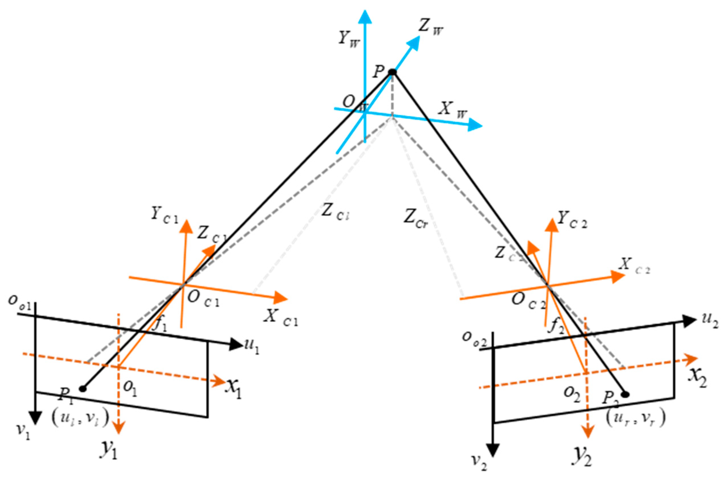
2.1. Infrared Binocular Camera Imaging Model

In an ideal scenario, the imaging model of a camera adheres to the pinhole camera model [30]. The typical imaging model for an infrared binocular camera is depicted in Figure 1.

In the schematic, the pixel coordinate systems on the imaging planes of two cameras are represented by $o_{o1}-u_1{v}_1$ and $o_{o1}-u_2{v}_2$. The physical coordinate systems of these imaging planes are denoted by $o_1-x_1{y}_1$ and $o_2-x_2{y}_2$. The camera coordinate systems for each camera, centered at the optical axes, are $O_{C1}-X_{C1}{Y}_{C1}{Z}_{C1}$ and $O_{C2}-X_{C2}{Y}_{C2}{Z}_{C2}$. The optical centers of the cameras are marked as $O_{C1}$ and $O_{C2}$, with focal lengths $f_1$ and $f_2$. The world coordinate system is designated by $O_W-X_W{Y}_W{Z}_W$. A feature point $P$ in 3D space has its Z-axis coordinates within the camera coordinate systems labeled as $Z_{Cl}$ and $Z_{Cr}$. The points $P_1$ and $P_2$ correspond to the projections of $P$ onto the imaging planes of the two cameras.

In the case of the left camera, the relationship (specifically, the affine transformation) between the physical image coordinate system and the pixel coordinate system is presented in Equation (1).

$$\left[\begin{array}{c}u\\ v\\ 1\end{array}\right]=\left[\begin{array}{ccc}{\displaystyle \frac{1}{dx}}& -{\displaystyle \frac{cot\phi }{dx}}& u_0\\ 0& {\displaystyle \frac{1}{dysin\phi }}& v_0\\ 0& 0& 1\end{array}\right]\left[\begin{array}{c}x\\ y\\ 1\end{array}\right]$$

(1)

In this context, $\left(u_0,v_0\right)$ signifies the coordinates of the physical image origin within the pixel coordinate system. The angle $\phi$, typically defaulted to zero, represents the angular separation between the detector’s edges.

The connection (specifically, the perspective projection transformation) between the camera coordinate system and the physical image coordinate system is detailed in Equation (2).

$$Z_C\left[\begin{array}{c}x\\ y\\ 1\end{array}\right]=\left[\begin{array}{ccc}f& 0& 0\\ 0& f& 0\\ 0& 0& 1\end{array}\right]\left[\begin{array}{c}{X}_C\\ Y_C\\ Z_C\end{array}\right]$$

(2)

In this equation, $f$ denotes the camera lens’s focal length.

The transformation between the world coordinate system and the camera coordinate system, known as the rigid body transformation, is depicted in Equation (3). Consequently, the pinhole camera model for the left infrared camera is established, as illustrated in Equation (4).

$$\left[\begin{array}{c}{X}_C\\ Y_C\\ Z_C\\ 1\end{array}\right]=\left[\begin{array}{cc}\mathit{R}& \mathit{T}\\ 0& 1\end{array}\right]\left[\begin{array}{c}{X}_W\\ Y_W\\ Z_W\\ 1\end{array}\right]$$

(3)

$$Z_C\left[\begin{array}{c}u\\ v\\ 1\end{array}\right]=\left[\begin{array}{cccc}{\displaystyle \frac{f}{dx}}& -{\displaystyle \frac{cot\theta }{dx}}& u_0& 0\\ 0& {\displaystyle \frac{f}{dysin\theta }}& v_0& 0\\ 0& 0& 1& 0\end{array}\right]\left[\begin{array}{cc}\mathit{R}& \mathit{T}\\ 0& 1\end{array}\right]\left[\begin{array}{c}{X}_W\\ Y_W\\ Z_W\\ 1\end{array}\right]=\mathit{K}\left[\begin{array}{cc}\mathit{R}& \mathit{T}\\ 0& 1\end{array}\right]\left[\begin{array}{c}{X}_W\\ Y_W\\ Z_W\\ 1\end{array}\right]$$

(4)

The matrix $\mathit{A}$ signifies the intrinsic parameters of the camera. The rotation matrix, denoted as $\mathit{R}$, and the translation matrix, denoted as $\mathit{T}$, collectively constitute the extrinsic matrix of the camera.

Beyond the intrinsic parameters and extrinsic parameters, the camera’s non-linear distortions [31], such as radial and tangential distortions, are vital parameters of the camera’s imaging model. Radial distortion is caused by the curvature of the optical lens, leading to rays bending inward or outward away from the optical axis, creating barrel or pincushion distortion, as formulated in Equation (5). Tangential distortion is due to the misalignment between the optical lens and the imaging plane of the sensor, detailed in Equation (6).

$$\left\{\begin{array}{c}{x}_{r_{distort}}=x\left(1+k_1{r}^2+k_2{r}^4+k_3{r}^6\right)\\ y_{r_{distort}}=y\left(1+k_1{r}^2+k_2{r}^4+k_3{r}^6\right)\end{array}\right.$$

(5)

$$\left\{\begin{array}{c}{x}_{t\_distort}=x+2p_{1}xy+p_2(r^2+2x^2)\\ y_{t\_distort}=y+p_1\left(r^2+2y^2\right)+2p_{2}xy\end{array}\right.$$

(6)

In this formula, $r^2=x^2+y^2$, where $(x,y)$ represent the coordinates of a point before distortion correction, and $(x_{distort},y_{distort})$ are the coordinates after the correction. The parameters $k_1,k_2,k_3$ correspond to the radial distortion coefficients, while $p_1,p_2$ are the tangential distortion coefficients.

Similarly, the intrinsic parameters and extrinsic parameters, along with the distortion coefficients, of the right infrared camera can be derived through analogous procedures.

For an infrared binocular system, the positional relationship between the two cameras is consistently stable. The relationship between the left camera’s coordinate system $O_{C1}-X_{C1}{Y}_{C1}{Z}_{C1}$ and the right camera’s coordinate system $O_{C2}-X_{C2}{Y}_{C2}{Z}_{C2}$ is established as Equation (7).

$$\left[\begin{array}{c}{X}_{C2}\\ Y_{C2}\\ Z_{C2}\end{array}\right]={\mathit{R}}_C\left[\begin{array}{c}{X}_{C1}\\ Y_{C1}\\ Z_{C1}\end{array}\right]+{\mathit{T}}_C$$

(7)

Based on Equations (3) and (7), the rotation matrix ${\mathit{R}}_C$ that transforms from the left camera coordinate system to the right is computed as ${\mathit{R}}_C={\mathit{R}}_2{\mathit{R}}_1^{-1}$. Similarly, the translation matrix ${\mathit{T}}_C$ for this transformation is given by ${\mathit{T}}_C={\mathit{T}}_2-{\mathit{R}}_2{\mathit{R}}_1^{-1}{\mathit{T}}_1$, with ${\mathit{R}}_1$, ${\mathit{T}}_1$ being the extrinsic parameters for the left camera, and ${\mathit{R}}_2,{\mathit{T}}_2$ being those for the right camera.

2.2. Principles and Steps for Camera Calibration and Optimization

Referring to the Formula (4) of the infrared camera’s imaging model, the precision of the infrared stereo camera calibration is primarily influenced by two factors, assuming that the chosen calibration approach—like the planar calibration method—is dependable. These critical factors are the precision of the pixel coordinates of the feature points and the precision of their corresponding world coordinates.

2.2.1. Optimization of Feature Point Pixel Coordinates

If there exists an angular disparity between the spatial circular plane and the detection plane, the circular plane target in three-dimensional space is imaged as an ellipse on the detection plane. Therefore, in the calibration process, the ellipse’s center is commonly extracted to approximate the imaging point of the circular target’s center. The precision of the ellipse detection significantly influences the accuracy of the feature point’s pixel coordinates, which can be enhanced by sub-pixel edge detection and optimization of ellipse fitting. Additionally, there exists an inherent discrepancy between the actual projection of the three-dimensional circular center and the determined center of the ellipse, which can be optimized by approximating the actual projection of the target’s center.

1.

Sub-pixel Edge Detection of Ellipse

Sub-pixel edge detection techniques significantly improve the precision of detecting the edges of circular targets in imaging, accurately pinpointing the center of the ellipse formed in the image. The images output by the infrared camera have been upsampled from the original to enhance detail. This study utilizes the sub-pixel edge estimation method for ellipses introduced by Lou Qun and colleagues [27], applying a quadratic function to approximate the local contour of the ellipse’s edge. The method estimates the parameters of the quadratic function by considering the area effect of the edge’s local region, thus achieving sub-pixel level edge estimation.

2.

Ellipse Fitting Optimization

Under optimal conditions, the major axes of the m×n standard circles, once imaged as ellipses on the target plane, should align in a uniform tilt angle. An initial estimation of the ellipses’ major axes tilt angles is conducted, followed by sorting of these angles. The average of the central (m × n)/2 angles is then selected to represent the tilt angle for the ellipses in each calibration image. Utilizing this angle, a RANSAC-based least squares optimization is performed to refine the fitting of the ellipse edges, yielding the precise center coordinates of the ellipses.

3.

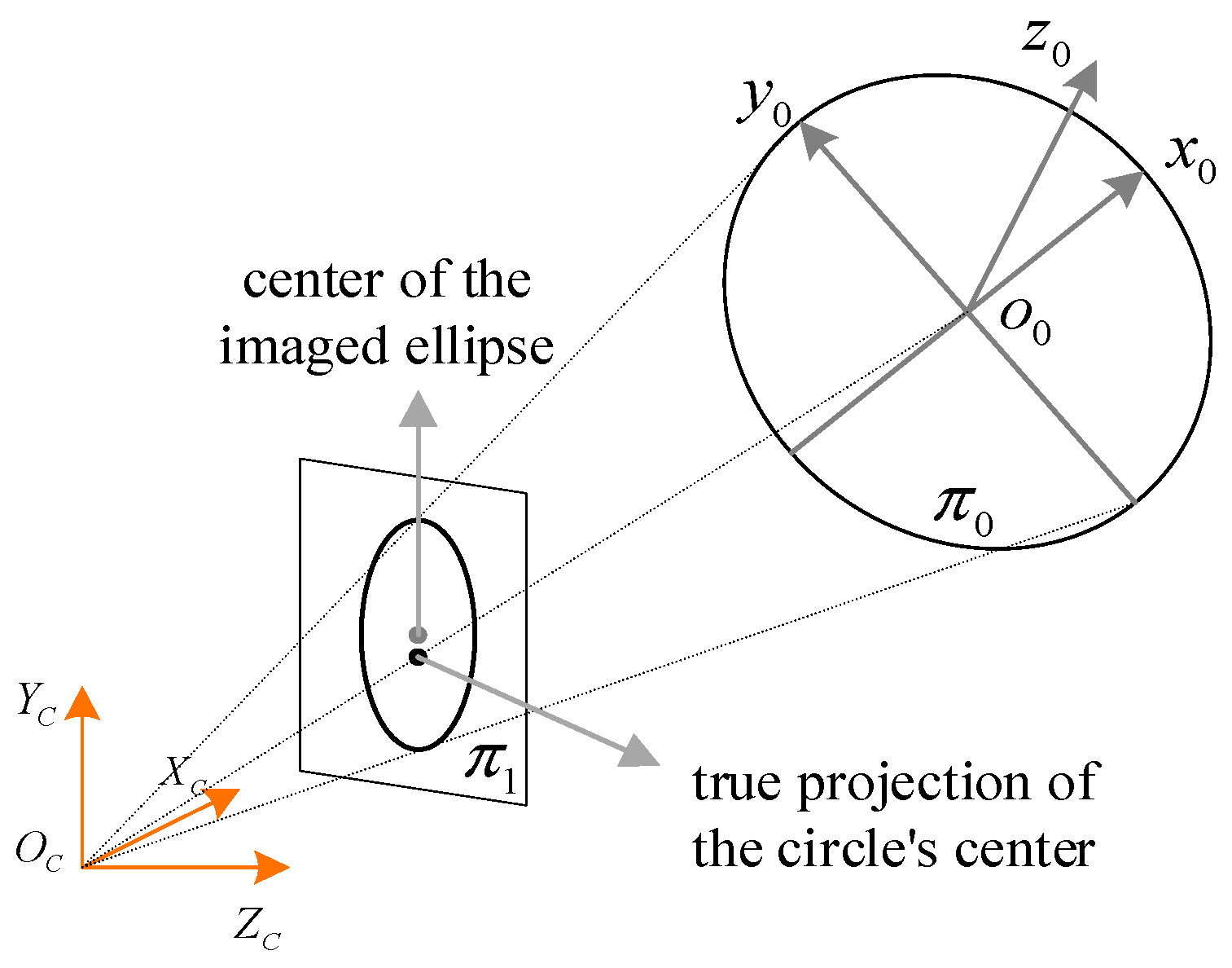
True Projection of the Target’s Actual Center

As per Equation (4), the imaging points of the target’s features are inversely projected back into three-dimensional space using the calibration parameters to generate a virtual calibration plane. The smaller the errors in the calibration parameters, the closer this virtual plane aligns with the actual physical calibration plane. Consequently, the sub-pixel edge of the ellipse, when inversely projected onto this virtual plane, exhibits minimal error relative to the true target’s circle. By performing an elliptical fit, we acquire the coordinates of the feature points on the virtual calibration plane and, upon reprojection onto the detector’s imaging plane, these points closely match the true projection of the target’s center.

2.2.2. Optimization of Feature Point World Coordinates

The circular target’s feature points have world coordinates ($X_W{,Y}_W,Z_W$), with the calibration method assuming the world coordinate system is fixed to the target plane, hence $Z_W$ equals zero. The coordinates ($X_W{,Y}_W$) for the m×n feature points are uniformly spaced according to the dimensions of the circular target. However, inherent manufacturing tolerances and potential minor distortions during calibration can impact the precision of the actual world coordinates of the feature points. The virtual target plane has a minimal angular difference from the real target plane. By conducting a least squares linear optimization on the circular center coordinates of the virtual target plane to ensure they align with the true target’s feature points’ alignment in both row and column directions, we derive the optimized world coordinates for the feature points.

2.2.3. Steps for Optimizing Camera Calibration

The workflow for optimizing feature point coordinates is depicted in Figure 2. The procedure for calibrating the infrared binocular camera is outlined below:

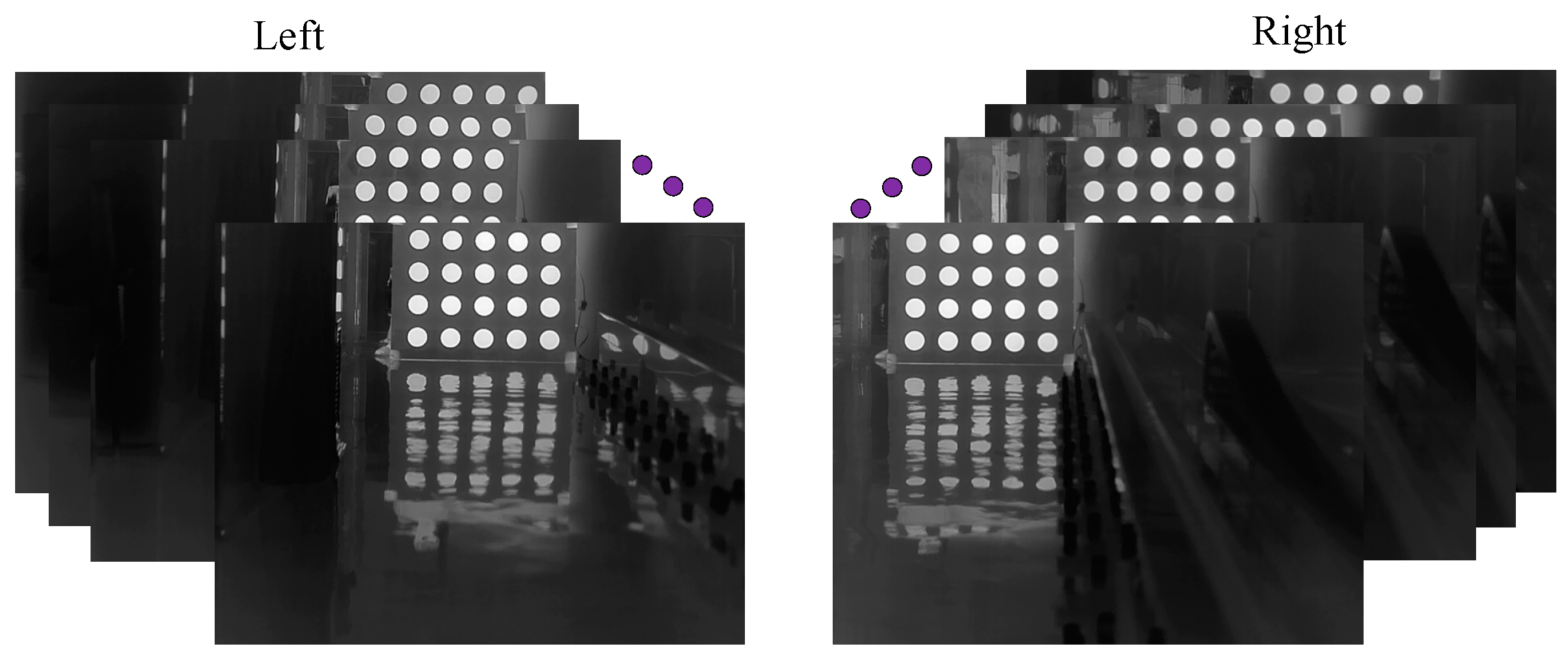
• In pursuit of improved camera calibration accuracy, the approach from reference [32] is adopted, focusing on altering the calibration board’s orientation by rotating it around the $X_W$ and $Y_W$ axes, instead of moving the board linearly or rotating it around the $Z_W$ axis. This method is complemented by the rotation of the infrared binocular camera setup to capture calibration images, ensuring that the target is captured across various positions in the combined field of view of both cameras, thus gathering an extensive set of valid calibration images. Utilizing a sub-pixel edge estimation technique for each image, the sub-pixel coordinates of the elliptical edges are extracted and subsequently refined to ascertain the central coordinates of the ellipses. The initial intrinsic and extrinsic parameters of the camera, along with the preliminary rotation and translation matrices relating the binocular camera coordinate systems, are calibrated using the planar calibration approach;
• Employing the preliminary values derived from the prior step, we calculate the coordinates in the camera coordinate system of the points where the centers of the ellipses are inversely projected into three-dimensional space, as per Equation (4). Ideally, these inverse projections fall within the plane of the actual target. Given that the initial errors from the planar calibration method are confined within acceptable limits, to approximate the true plane more accurately and minimize the effects of noise, we utilize the RANSAC to eliminate outlier points with significant deviations of the inverse projections. The equation of the virtual plane in the camera’s coordinate system is thereby established through the least squares method;
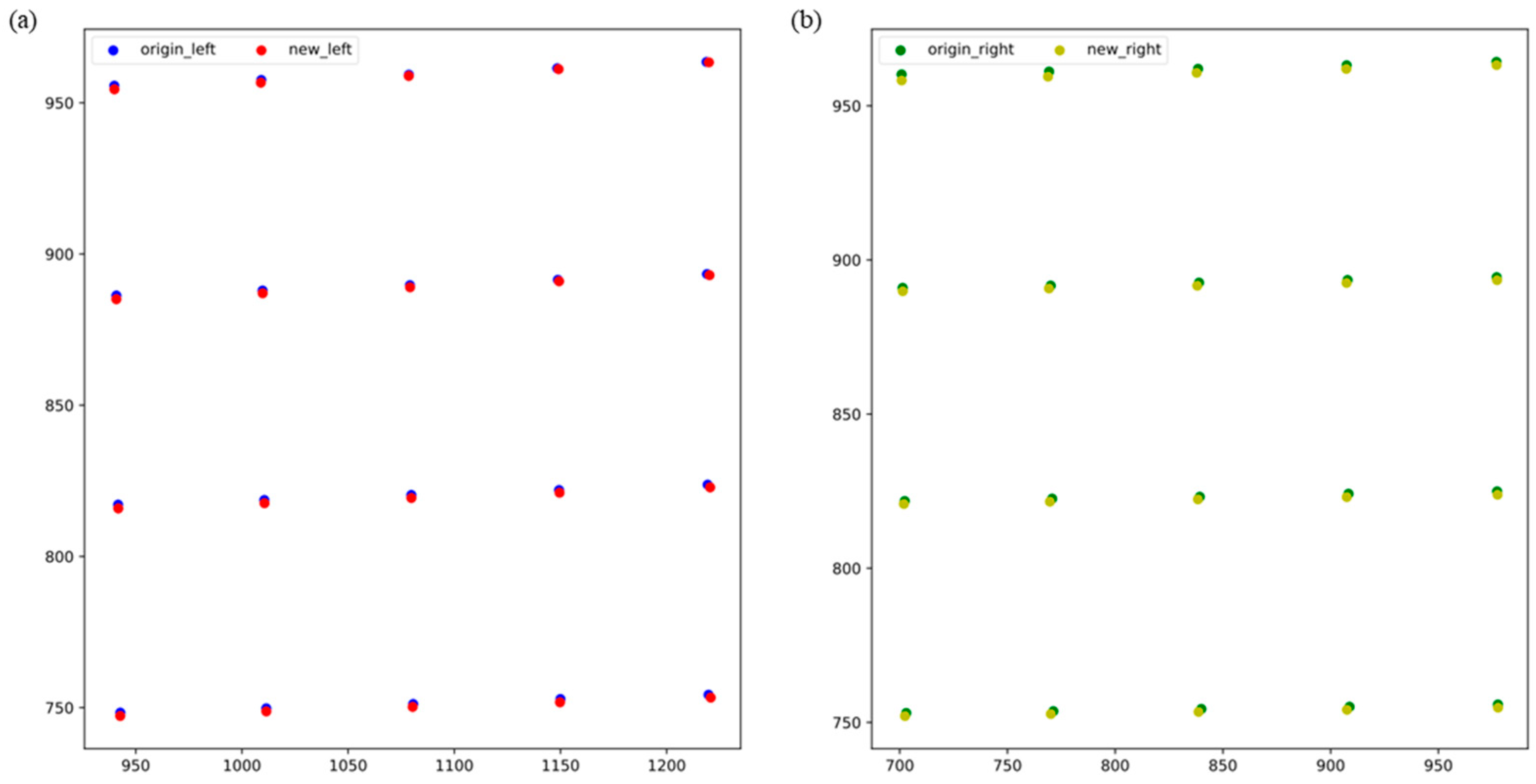
• Given that there is inherent discrepancy between the coordinates of the true target’s center as imaged and the coordinates of the extracted ellipse center, the process involves inversely projecting the ellipse edges onto the virtual target plane. An elliptical fit is then applied to the features on this virtual plane, and a least squares linear optimization is conducted on the central feature points of the ellipse. This methodology results in obtaining the feature points aligned with the world coordinates;
• By reprojecting the refined feature points onto the image plane and leveraging the pixel coordinates of these projections along with their corresponding world coordinates, a re-calibration of the plane is performed to determine the ultimate calibration parameters for the infrared camera. Thereafter, the transformation parameters between the two infrared binocular cameras are acquired through the application of stereo calibration algorithms.

2.3. Error Analysis

Throughout the calibration procedure of binocular infrared cameras, the errors can be attributed to three main sources: inaccuracies in the world coordinates of the feature points, imprecision in the pixel coordinates of these feature points, and discrepancies introduced by the calibration methodology itself.

2.3.1. Feature Point World Coordinate Error

Errors in the world coordinates of feature points, which equate to the errors of the calibration board’s feature points, are primarily attributed to machining inaccuracies and the thermal deformation of aluminum alloy plates, with the former being contingent upon the precision of the manufacturing process.

As for the thermal deformation errors of the aluminum alloy plates, the assumption is that the heating plate provides uniform heat and the metal plate undergoes uniform thermal expansion, in accordance with Fourier’s law of heat conduction [33] (as in Equation (8)).

$$q=-k·S·{\displaystyle \frac{∆T}{∆x}}$$

(8)

Here, $S$ denotes the area through which heat is conducted, $k$ refers to the material’s thermal conductivity, $q$ signifies the heat flux through area $S$, $∆T$ is the temperature differential across the metal plate, and $∆x$ indicates the distance or thickness along which heat is transmitted.

Furthermore, the convective heat transfer formula, exemplified by Equation (9), delineates the thermal interaction between a solid surface and the enveloping fluid.

$$q=h_c·S·(T_s-T_{\infty })$$

(9)

In this equation, $h_c$ denotes the convective heat transfer coefficient, $T_s$ represents the temperature of the solid surface, and $T_{\infty }$ signifies the temperature of the fluid at a distance from the solid surface.

The curvature and elongation of a metal plate due to thermal expansion can be precisely quantified through the application of Equations (10) and (11).

$$ϵ={\displaystyle \frac{\alpha \times ∆T}{h}}$$

(10)

$$∆L=\alpha \times L_0\times ∆T$$

(11)

In this formula, $ϵ$ denotes the curvature of the metal plate, $\alpha$ refers to the metal’s coefficient of thermal expansion, $∆T$ indicates the temperature differential across the plate, $h$ is the thickness of the metal plate, $∆L$ signifies the change in length of the object, and $L_0$ is the original length.

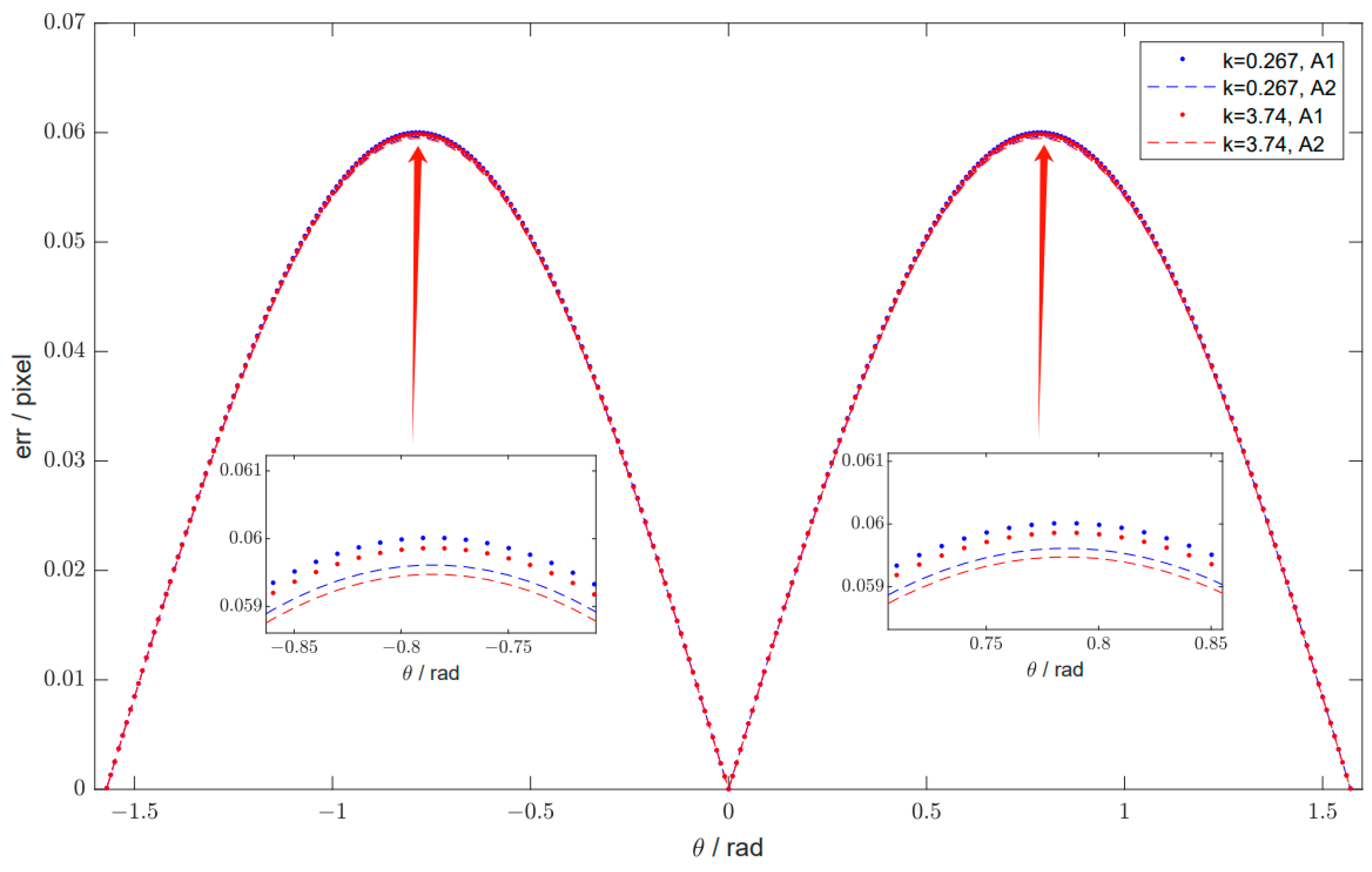
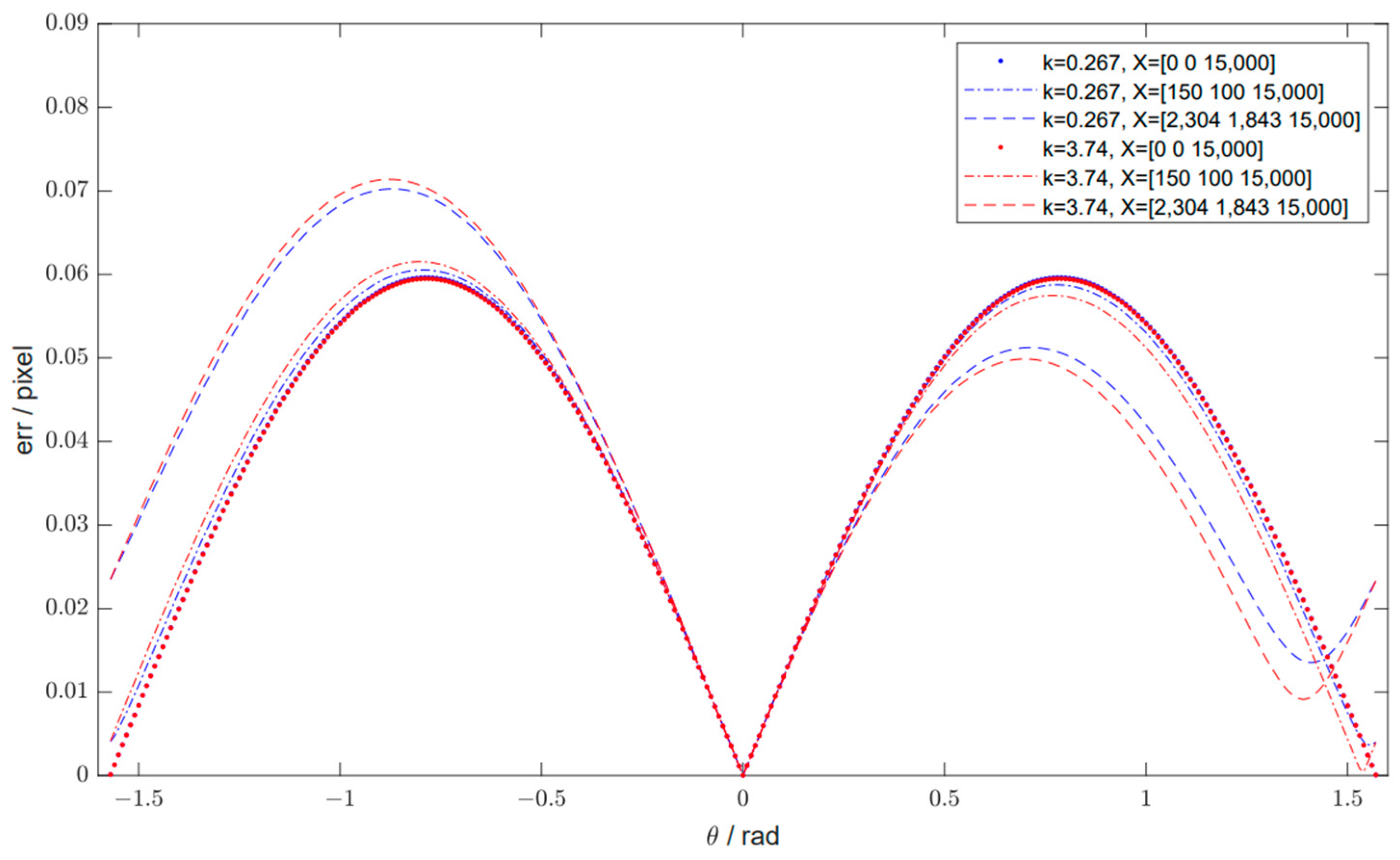
2.3.2. Feature Point Pixel Coordinate Error

The inaccuracies in the pixel coordinates of feature points, specifically the deviations in identifying the projected points of the calibration board’s circular centers, can be attributed to two primary sources of error: projection distortion and the inaccuracies in determining the center of the ellipse. The latter are contingent upon the algorithm used for extraction, whereas the former arises from discrepancies between the true projection of the circular centers in three-dimensional space and the actual centers of the projected ellipses.

Figure 3 illustrates the spatial circular plane imaging model, where ${\pi }_0$ denotes the spatial circular plane and ${\pi }_1$ represents the camera’s imaging plane. $O_C-X_C{Y}_C{Z}_C$ signifies the camera coordinate system, and $o_0-x_0{y}_0$ indicates the coordinate system of the spatial circular plane. $z_0$ is the unit normal vector of the spatial circular plane ${\pi }_0$. Define $z_0=(cos\alpha , cos\beta , cos\theta )$, where α, β, and θ are the angles between the $z_0$ vector and each of the coordinate axes of the camera coordinate system, respectively, and ${cos}^2\alpha +{cos}^2\beta +{cos}^2\theta =1$.

Drawing from reference [34], the relationship between the camera’s image plane ${\pi }_1$ and the circular plane ${\pi }_0$ is formulated as Equation (12).

$$s{X}_1=H{X}_0$$

(12)

In this equation, $s$ is a scalar constant, $X_1$ is the projected coordinate on the image plane of a point located on the circular plane ${\pi }_0$, $X_0$ is the homogeneous coordinate of a point on the circular plane ${\pi }_0$ within the two-dimensional coordinate system ${o_0-x}_0{y}_0$, and H is a 3 × 3 matrix derived from the camera’s intrinsic matrix and the transformation matrix from the camera coordinate system $O_C-X_C{Y}_C{Z}_C$ to the coordinate system ${o_0-x}_0{y}_0{z}_0$.

$$H=\left[\begin{array}{ccc}{q}_{11}& q_{12}& q_{13}\\ q_{21}& q_{22}& q_{23}\\ q_{31}& q_{32}& q_{33}\end{array}\right]$$

(13)

The equation of the spatial circular plane curve $X_0^T{B}_0{X}_0=0$ correlates with the equation of the projected elliptical curve on the image plane $X_1^T{B}_1{X}_1=0,$ as Equation (14).

$$B_1=k{\left(H^{-1}\right)}^T{B}_0{H}^{-1}$$

(14)

In this context, k denotes a constant value.

$$B_0=\left[\begin{array}{ccc}1/a^2& 0& 0\\ 0& 1/a^2& 0\\ 0& 0& -1\end{array}\right], B_1=\left[\begin{array}{ccc}{b}_1& b_2/2& b_4/2\\ b_2/2& b_3& b_5/2\\ b_4/2& b_5/2& b_6\end{array}\right]$$

(15)

Within the formula, a denotes the radius of the circle in space, while $\left(b_1,b_2,b_3,b_4,b_5,b_6\right)$ correspond to the coefficients of the projected ellipse.

The projection distortion error is quantified by the distance between the center of the ellipse $X_1\left(O_1\right)$) and the actual projection of the center of the circle $X_1\left(O_2\right)$, as in Equation (16).

$$d_{err}=\sqrt{{({\displaystyle \frac{2b_3{b}_4-b_2{b}_5}{b_2^2-4b_1{b}_3}}-{\displaystyle \frac{q_{13}}{q_{33}}})}^2+{({\displaystyle \frac{2b_1{b}_5-b_2{b}_4}{b_2^2-4b_1{b}_3}}-{\displaystyle \frac{q_{23}}{q_{33}}})}^2}$$

(16)

2.3.3. Calibration Error

Calibration error, synonymous with reprojection error [35], is determined through the calibration process.

2.4. Infrared Binocular Ranging

The traditional binocular ranging principle [36], relies on parameters derived from camera calibration to achieve stereo rectification, aligning the binocular system with ideal conditions. The formula for ideal binocular ranging, presented in Equation (17), defines $f$ as the focal length of the camera, $B$ as the baseline distance between the optical centers of the two cameras, and $d$ as the disparity of the spatial target as captured by the stereo pair.

$$D={\displaystyle \frac{f·B}{d}}$$

(17)

This process involves a transformation that projects the images from both cameras onto a unified plane, ensuring that the epi-polar lines of the left and right camera images are aligned horizontally. With these rectified and refined parameters, the distance to corresponding feature points is calculated using the triangulation formula. However, the stereo rectification transformation [37] may lead to the loss of pixel data from the original camera images. In this study, we bypass this potential data loss by directly ranging targets in the original images captured by both the left and right cameras. The underlying principle of this direct ranging approach is outlined below.

Suppose the left camera is designated as the primary camera, and we typically concentrate on the coordinates of spatial feature points within its coordinate system. For any arbitrary point P in 3D space, its coordinates in the left camera’s coordinate system are $(X,Y,Z)$, and the corresponding projection points on the image planes of the left and right cameras are $(u_l,v_l)$ and $(u_r,v_r)$, respectively. Post-calibration, the projection matrix for point $P$ in the left camera is denoted as ${\mathit{M}}_l$, and for the right camera, it is ${\mathit{M}}_r$, from which we derive Equation (18):

$$\left\{\begin{array}{c}{Z}_{Cl}\left[\begin{array}{c}{u}_l\\ v_l\\ 1\end{array}\right]={\mathit{M}}_l\left[\begin{array}{c}\begin{array}{c}X\\ Y\end{array}\\ Z\\ 1\end{array}\right]\\ Z_{Cr}\left[\begin{array}{c}{u}_r\\ v_r\\ 1\end{array}\right]={\mathit{M}}_r\left[\begin{array}{c}\begin{array}{c}X\\ Y\end{array}\\ Z\\ 1\end{array}\right]\end{array}\right.$$

(18)

Here, $Z_{Cl}$ and $Z_{Cr}$ represent the Z-axis coordinates of spatial point $P$ in the left and right camera coordinate systems, respectively.

$$\left\{\begin{array}{c}{\mathit{M}}_l={\mathit{K}}_l\left[\begin{array}{cc}\mathit{I}& \mathbf{0}\\ 0& 0\end{array}\right]=\left[\begin{array}{ccc}{m}_{11}& m_{12}& \begin{array}{cc}{m}_{13}& m_{14}\end{array}\\ m_{21}& m_{22}& \begin{array}{cc}{m}_{23}& m_{24}\end{array}\\ m_{31}& m_{32}& \begin{array}{cc}{m}_{33}& m_{34}\end{array}\end{array}\right]\\ {\mathit{M}}_r={\mathit{K}}_r\left[\begin{array}{cc}{\mathit{R}}_C& {\mathit{T}}_C\\ 0& 0\end{array}\right]=\left[\begin{array}{ccc}{n}_{11}& n_{12}& \begin{array}{cc}{n}_{13}& n_{14}\end{array}\\ n_{21}& n_{22}& \begin{array}{cc}{n}_{23}& n_{24}\end{array}\\ n_{31}& n_{32}& \begin{array}{cc}{n}_{33}& n_{34}\end{array}\end{array}\right]\end{array}\right.$$

(19)

Substitute ${\mathit{M}}_{\mathit{l}}$ and ${\mathit{M}}_{\mathit{r}}$ into Equation (19), respectively, and then simplify to obtain Equation (20).

$$\left\{\begin{array}{c}\left(u_l{m}_{31}-m_{11}\right)X+\left(u_l{m}_{32}-m_{12}\right)Y+\left(u_l{m}_{33}-m_{13}\right)Z=m_{14}-u_l{m}_{34}\\ \left(v_l{m}_{31}-m_{21}\right)X+\left(v_l{m}_{32}-m_{22}\right)Y+\left(v_l{m}_{33}-m_{23}\right)Z=m_{24}-v_l{m}_{34}\\ \begin{array}{c}\left(u_r{n}_{31}-n_{11}\right)X+\left(u_r{n}_{32}-n_{12}\right)Y+\left(u_r{n}_{33}-n_{13}\right)Z=n_{14}-u_r{n}_{34}\\ \left(v_r{n}_{31}-n_{21}\right)X+\left(v_r{n}_{32}-n_{22}\right)Y+\left(v_r{n}_{33}-n_{23}\right)Z=n_{24}-v_r{n}_{34}\end{array}\end{array}\right.$$

(20)

In an ideal stereo vision model, the above equation has a unique solution, but in practical applications, it represents an overdetermined system of equations, which is typically solved for the best fit using the least squares method. The equation, when expressed in matrix form, is as shown in Equation (21).

$$\mathit{B}\mathit{X}=\mathit{G}$$

(21)

Thus, the optimal solution for the coordinates of spatial point $P$ can be expressed by Equation (22).

$$\mathit{X}={\left({\mathit{B}}^T\mathit{B}\right)}^{-1}{\mathit{B}}^T\mathit{G}$$

(22)

Here, $\mathit{X}={\left[\begin{array}{ccc}X& Y& Z\end{array}\right]}^T$.

$$\mathit{B}=\left[\begin{array}{ccc}{u}_l{m}_{31}-m_{11}& u_l{m}_{32}-m_{12}& u_l{m}_{33}-m_{13}\\ v_l{m}_{31}-m_{21}& v_l{m}_{32}-m_{22}& v_l{m}_{33}-m_{23}\\ \begin{array}{c}{u}_r{n}_{31}-n_{11}\\ v_r{n}_{31}-n_{21}\end{array}& \begin{array}{c}{u}_r{n}_{32}-n_{12}\\ v_r{n}_{32}-n_{22}\end{array}& \begin{array}{c}{u}_r{n}_{33}-n_{13}\\ v_r{n}_{33}-n_{23}\end{array}\end{array}\right], \mathit{G}=\left[\begin{array}{c}{m}_{14}-u_l{m}_{34}\\ m_{24}-v_l{m}_{34}\\ \begin{array}{c}{n}_{14}-u_r{n}_{34}\\ n_{24}-v_r{n}_{34}\end{array}\end{array}\right]$$

(23)

With the left camera designated as the primary camera, the coordinate $Z$ of point $P$ in the left camera’s coordinate system is transformed into the formula representing the distance from the spatial point to the center of the left camera’s aperture (the origin of the camera coordinate system), as depicted in Equation (24).

$$D=Z·{\displaystyle \frac{\sqrt{{(u_l-u_0)}^2+{(v_l-v_0)}^2+f_l^2}}{f_l}}$$

(24)

3. Experiments and Results

This section is divided into three parts: calibration preparation, calibration experiment and error analysis, and distance measurement and error analysis, providing a detailed description of the calibration and distance measurement experiments of the infrared binocular target ranging system.

3.1. Preparations for Infrared Binocular Camera Calibration

The infrared binocular camera setup employs a pair of identical infrared cameras, detailed parameters of which are presented in

Table 1. Parameters of infrared camera.

Effective Focal Length	25 mm
Field Of View (640 * 512)	17.6° (H) × 14.1° (V)
Wavelength band	8~12 $\mathsf{\mu }\mathrm{m}$
F-Number	1.0
pixel size	12 $\mathsf{\mu }\mathrm{m}$
aperture diameter (D)	25 mm

. Secured in a horizontal alignment on an aluminum plate, the cameras are spaced 1 m apart, with the physical setup illustrated in Figure 4.

Custom-designed for the infrared binocular camera system, a calibration target was fabricated with dimensions of 1.5 m in length, 1.2 m in width, and 5 mm in thickness. The target features a 4 × 5 grid of circular spots, each with a diameter of 16 cm and spaced 27 cm apart from the center of one circle to the center of the next, as depicted in Figure 5. The rear side of the calibration board is affixed to a silicone heating pad using 3 M (Minnesota Mining and Manufacturing Company) adhesive.

3.2. Infrared Binocular Camera Calibration Experiment

Reprojection error [20] is the difference between the actual image points of spatial features and the points projected by the mathematical model and calibration parameters. The mean reprojection error, which is the average of the reprojection errors for all feature points, serves as a crucial indicator of camera calibration accuracy.

In accordance with the calibration procedures, this study captured 84 sets of valid calibration images for the left and right cameras at a distance of approximately 15 m, with selected examples illustrated in Figure 6. The choice of target distance is informed by preliminary calculations and experimental findings.

Utilizing the algorithm detailed in this paper, the sub-pixel edges of the circular images from each calibration image are determined through RANSAC least squares fitting to form ellipses with consistent major axis inclinations, as depicted in Figure 7. The blue curve on the right indicates the ellipse fit from all edge points, while the red curve shows the optimized ellipse. The yellow coordinate points signify the outliers eliminated by the RANSAC algorithm. Based on the optimized coordinates of the ellipse centers, initial values for the internal and external parameters and distortion parameters of the two cameras are obtained using the planar calibration method. Subsequently, stereo calibration is conducted to determine the rotational and translational matrices that describe the spatial relationship between the two cameras.

The results of the inverse projection of the imaging ellipse centers into three-dimensional space with the initial calibration parameters are illustrated in Figure 8a. Utilizing RANSAC to eliminate points with significant optimization errors on the plane, a virtual target plane is derived from the remaining spatial points through least squares fitting, as shown in Figure 8b. Following this, the edges of the imaging ellipses are inversely projected onto the virtual target plane, and the centers of the ellipses, as fitted within this plane, are reprojected onto the imaging plane. Figure 9 displays these outcomes, with the original ellipse centers in the left camera’s image marked by blue dots and the reprojected points by red dots; similarly, the green dots in the right camera’s image indicate the original ellipse centers, with yellow dots representing the reprojected points.

By reprojecting the feature points, the calibration is reiterated. A comparison between the final calibration outcomes of this study and those obtained directly by the traditional planar calibration method is presented in

Table 2. Comprehensive calibration results.

Approach	fx	Fy	u0	v0	Reprojection Error
T.(l)	4208.272	4220.292	638.959	444.632	0.025472
T.(r)	4191.947	4204.317	665.182	439.508	0.025529
P.(l)	4170.279	4180.970	631.355	489.283	0.019233 (−24.5%)
P.(r)	4166.903	4177.129	675.926	491.014	0.019351 (−24.2%)

,

Table 3. Camera distortion parameters.

Approach	k1	k2	k3	p1	p2
T.(l)	0.10974	0.66015	12.30672	−0.00747	0.00045
T.(r)	0.12118	0.04299	6.32299	−0.01042	0.00115
P.(l)	0.08885	1.24429	−7.72630	−0.00178	−0.00016
P.(r)	0.10674	−0.31974	15.73494	−0.00413	0.00219

and

Table 4. Stereo camera rotation matrix and translation matrix.

Approach	RC	TC	res
T.	[[0.9999396  0.0106574  −0.0026880] [−0.0106500  0.9999396  0.0027297] [0.0027169  −0.0027009  0.9999927]]	[[−102.1816259] [0.49134853] [−6.83686545]]	0.450877
P.	[[ 0.999922  0.0101889  −0.0071329] [−0.0101816  0.9999476  0.0010583] [0.0071433  −0.0009856  0.9999740]]	[[−102.00134939] [0.57938219] [−2.972963]]	0.438399 (−2.8%)

. The abbreviations T.(l) and T.(r) correspond to the traditional calibration results for the left and right cameras, respectively, while P.(l) and P.(r) signify the results from the method introduced in this paper. The findings demonstrate that the proposed calibration technique has an average reprojection error of less than 0.02 pixels, which is a 24.5% improvement over the conventional approach, thereby effectively increasing the precision of camera calibration.

Based on the results of the proposed calibration method, after stereo rectification, the updated parameters are presented in

Table 5. Parameters after stereoscopic correction.

Parameters	Values
A1′	[[4.08556674 × 103  0.00000000  5.34163437 × 102  0.00000000] [0.00000000  4.08556674 × 103  4.89555637 × 102  0.00000000] [0.00000000  0.00000000  1.00000000  0.00000000]]
A2′	[[4.08556674 × 103  0.00000000  5.34163437 × 102  4.23220829 × 105] [0.00000000  4.08556674 × 103  4.89555637 × 102  0.00000000] [0.00000000  0.00000000  1.00000000  0.00000000]]
RC′	[[1.00000000  9.22250370 × 10−12  1.44598916 × 10−12] [9.23272358 × 10−12  1.00000000  1.75414967 × 10−12] [1.43979273 × 10−12  1.75546004 × 10−12  1.00000000]]
TC′	[[−1.03589259 × 102] [−8.54871729 × 10−15] [ 3.63530766 × 10−13]]

. A1′ and A2′ represent the intrinsic parameters of the two cameras after rectification, while RC′ and TC′ denote the rotation matrix and translation matrix between the two cameras post-rectification, respectively. After stereo rectification, the intrinsic parameters of both cameras are identical, indicating that TC′ shows only a horizontal displacement between the cameras with negligible deviation in other directions. RC′ indicates that there is almost no rotational angle between the cameras, which confirms the accuracy of the calibration results.

The comparison between the left and right camera images before and after stereo rectification is illustrated in Figure 10. The designed and installed infrared binocular camera has achieved a commendable level of parallelism, rendering the visual distinction between the left and right images subtle without stereo correction. Nevertheless, discrepancies persist, discernible through the detailed features highlighted in red and blue circles in Figure 10a. The stereo-corrected image pairs, illustrated in Figure 10b, exhibit notably enhanced parallelism.

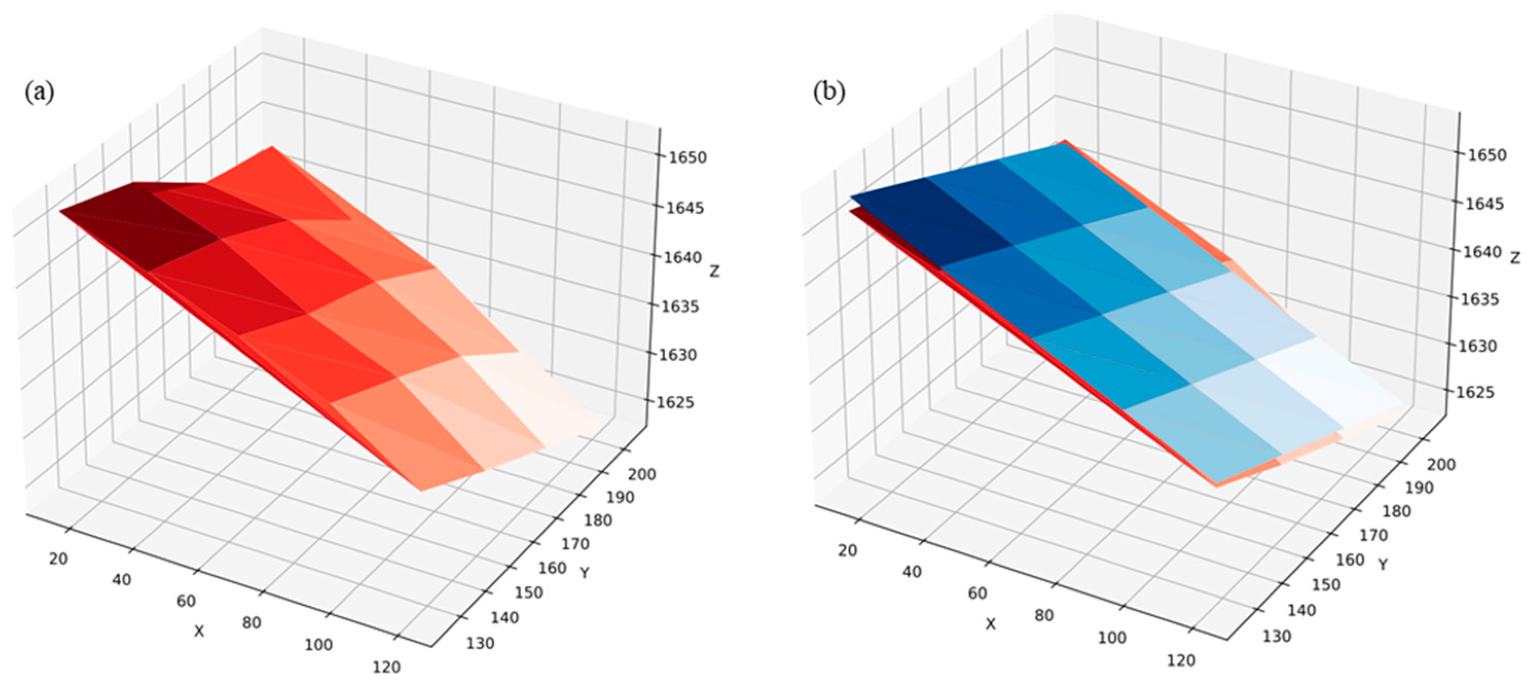
3.3. Results of Error Analysis

The camera calibration outcomes indicate that the calibration errors for both the left and right infrared cameras are 0.019 pixels. The manufacturing precision of the calibration board is kept under 1mm, translating to a pixel plane error of about 0.14 pixels on the infrared camera at a 15-m distance. Simulation results from reference [6] suggest that the ellipse center extraction error remains below 1.4 pixels across various noise levels.

Employing the formula for calculating the thermal deformation of metal plates, for an aluminum alloy plate ($k=138 \mathrm{W}/(\mathrm{m}·\mathrm{K})$, $\alpha =23.8\times {10}^{-6}{/}^{\circ }\mathrm{C}$) under ambient conditions of 25 °C (air temperature during the calibration experiment) with a gentle breeze ($h_C=25 \mathrm{W}/({\mathrm{m}}^2·\mathrm{K})$), the maximum depth error at the edge when uniformly heated to 50 °C via a heating plate is 0.03 mm, while the errors in the length and width directions are less than 0.001 mm, negligible for practical purposes.

As for projection distortion errors, Figure 11 depicts the relationship between distortion error and $\theta$ when the center of the spatial circular plane is on the optical axis $Z_C$, with $cos\alpha =kcos\beta$ (where k is any constant). At this juncture, distortion errors peak at $\theta =\pm {\displaystyle \frac{\pi }{4}}$, with the peak positions being unaffected by the value of k. $A_1$ and $A_2$ denote the intrinsic parameters of the camera for planar calibration method and the proposed method, respectively. The proposed method yields calibration parameters that exhibit a lower degree of error in projection distortion.

Figure 12 illustrates the relationship between distortion error and θ as the center of the spatial circular plane moves away from the optical axis, based on the optimized calibration parameters. Here, X denotes the coordinates of the circular plane’s center in the camera’s coordinate system, measured in millimeters. A value of X = [0 0 15,000] signifies alignment with the optical axis, X = [150 100 15,000] suggests a minor deviation, and X = [2304 1843 15,000] indicates a substantial angular displacement from the axis. The experimental infrared camera’s maximum planar center deviation corresponds to X = [2304 1843 15,000]. The graph reveals that increased deviation of the circular plane’s center from the optical axis correlates with higher maximum projection distortion errors.

Figure 13 demonstrates the relationship between distortion error and the distance d from the center of the spatial circular plane to the camera’s $X_C{O}_C{Y}_C$ plane when the center is off-axis. The notation X = 0 signifies that the center is aligned with the optical axis, while X = near and X = far denote minor and significant off-axis deviations, respectively. The graph shows that the projection distortion error decreases sharply initially and then reduces more slowly as the distance d increases.

Integrating the simulation findings, the circular plane’s center exhibits a maximum projection distortion of around 0.07 pixels at a distance of 15 m from the infrared camera. All error statistics are summarized in

Table 6. Error statistics.

	World Coordinate Error		Pixel Coordinate Error		Calibration Error
	Machining Inaccuracies	Thermal Deformation	Projection Distortion	Center Extraction Error
Error/pixel	<0.14	~0	<0.07	<1.4	0.019

.

3.4. Infrared Binocular Camera Ranging Experiment

Infrared binocular data for a circular metal plate were gathered at a range of distances, and the imaging center coordinates of the metal plate were extracted. The distance from the metal plate’s center to the center of the left camera’s pupil was then computed according to Equation (23). A comparison with traditional binocular ranging outcomes is presented in

Table 7. Infrared binocular camera ranging results.

Actual Distance/m	Direct Ranging/m (Relative Error/%)	Ranging after Rectification/m (Relative Error/%)
11.52	11.50 (−0.17)	11.55 (+0.26)
16.38	16.24 (−0.85)	16.26 (−0.73)
22.51	22.19 (−1.42)	21.90 (−2.71)
34.57	35.63 (+3.07)	40.55 (+17.30)
44.02	45.79 (+4.02)	49.63 (+12.74)
55.16	52.50 (−4.82)	55.65 (+0.89)

, with the actual distance being determined by a laser rangefinder from the metal plate’s center to the left camera. The findings indicate that the directly ranging method achieves greater precision and robustness in ranging compared to ranging after stereo rectification, maintaining an error margin of less than 5% within the 55-m range. The increased ranging errors and reduced robustness observed after stereoscopic calibration could be attributed to the transformation process, which may lead to the loss of certain pixel points and alterations in the target’s image geometry.

According to Equation (17), the calculation of the ranging error for an ideal binocular camera is detailed in Equation (25), with $∆D$ denoting the ranging error and $∆d$ signifying the disparity error. Consequently, Equation (26) illustrates the calculation of the relative ranging error, which exhibits a linear relationship with the actual distance to the target. The experimental binocular camera should maintain similar characteristics.

$$∆D={\displaystyle \frac{\partial D}{\partial d}}∆d=-{\displaystyle \frac{f·B}{d^2}}∆d=-{\displaystyle \frac{D^2}{f·B}}∆d$$

(25)

$${\displaystyle \frac{\left|∆D\right|}{D}}={\displaystyle \frac{D}{f·B}}\left|∆d\right|$$

(26)

Figure 14 illustrates the relationship between the absolute values of the relative errors from the direct ranging results in Table 7 and the actual target distances. The graph indicates that, as distance increases, the relative ranging error tends to vary linearly, aligning with theoretical expectations. However, given the significant deviation and poor robustness of the ranging error post-calibration, an in-depth analysis is not conducted.

4. Conclusions

Infrared cameras, leveraging their distinctive benefits, are increasingly being integrated across diverse applications. Recognizing the limitations in precision when calibrating infrared cameras with conventional methods, this paper introduces a high-precision calibration technique specifically for infrared binocular cameras, utilizing a custom circular planar target. This technique focuses on optimizing two key factors that impact the calibration of camera parameters: the pixel coordinates of feature points and their corresponding world coordinates. Initially, sub-pixel edge estimation is employed to capture the imaging edges of the target’s circles, followed by the application of the RANSAC least squares method to refine the imaging ellipses. The centers of these imaging ellipses are then back-projected into three-dimensional space, and the RANSAC least squares method is applied once more to optimize the back-projected points and establish a virtual target plane. Subsequently, the imaging edges of the target circles are back-projected onto this virtual target plane to derive feature points of the circle centers within the plane. These points are further refined through linear optimization to approximate their real-world coordinates. Finally, the feature points on the virtual target plane are reprojected onto the imaging plane, yielding optimized pixel coordinates for the feature points, which are then used for the calibration of the infrared camera. The calibration experiments demonstrate that the proposed approach, compared to the traditional planar calibration method, achieves a 24.5% reduction in average reprojection error, significantly improving the precision of infrared camera calibration and fulfilling the criteria for high-accuracy calibration needs. In addition, this paper has conducted an in-depth analysis of the errors in the calibration process and has achieved high-precision long-distance ranging with the infrared binocular camera, which is of great significance for the accurate detection and obstacle avoidance of targets in dark and other adverse environments.

References

1. Bao, D.; Wang, P. Vehicle distance detection based on monocular vision. In Proceedings of the 2016 International Conference on Progress in Informatics and Computing (PIC), Shanghai, China, 23–25 December 2016; pp. 187–191. [Google Scholar]
2. Chwa, D.; Dani, A.P.; Dixon, W.E. Range and motion estimation of a monocular camera using static and moving objects. IEEE Trans. Control Syst. Technol. 2015, 24, 1174–1183. [Google Scholar] [CrossRef]
3. Ferrara, P.; Piva, A.; Argenti, F.; Kusuno, J.; Niccolini, M.; Ragaglia, M.; Uccheddu, F. Wide-angle and long-range real time pose estimation: A comparison between monocular and stereo vision systems. J. Vis. Commun. Image Represent. 2017, 48, 159–168. [Google Scholar] [CrossRef]
4. Huang, L.; Zhe, T.; Wu, J.; Wu, Q.; Pei, C.; Chen, D. Robust inter-vehicle distance estimation method based on monocular vision. IEEE Access 2019, 7, 46059–46070. [Google Scholar] [CrossRef]
5. Li, W.; Shan, S.; Liu, H. High-precision method of binocular camera calibration with a distortion model. Appl. Opt. 2017, 56, 2368–2377. [Google Scholar] [CrossRef] [PubMed]
6. Xicai, L.; Qinqin, W.; Yuanqing, W. Binocular vision calibration method for a long-wavelength infrared camera and a visible spectrum camera with different resolutions. Opt. Express 2021, 29, 3855–3872. [Google Scholar] [CrossRef]
7. Liu, F.; Lu, Z.; Lin, X. Vision-based environmental perception for autonomous driving. Proc. Inst. Mech. Eng. Part D J. Automob. Eng. 2023, 0, 09544070231203059. [Google Scholar] [CrossRef]
8. Wang, J.; Geng, K.; Yin, G.; Cheng, X.; Sun, Y.; Ding, P. Binocular Infrared Depth Estimation Based On Generative Adversarial Network. In Proceedings of the 2022 6th CAA International Conference on Vehicular Control and Intelligence (CVCI), Nanjing, China, 28–30 October 2022; pp. 1–6. [Google Scholar]
9. Li, H.; Wang, S.; Bai, Z.; Wang, H.; Li, S.; Wen, S. Research on 3D reconstruction of binocular vision based on thermal infrared. Sensors 2023, 23, 7372. [Google Scholar] [CrossRef] [PubMed]
10. Su, B.; Gong, Y.; Yu, S.; Li, H.; Wang, Z.; Liu, W.; Wang, J.; Kuang, S.; Yao, W.; Tang, J. 3D spatial positioning by binocular infrared cameras. In Proceedings of the 2021 WRC Symposium on Advanced Robotics and Automation (WRC SARA), Beijing, China, 11 September 2021; pp. 67–72. [Google Scholar]
11. Wang, Z.; Liu, B.; Huang, F.; Chen, Y.; Zhang, S.; Cheng, Y. Corners positioning for binocular ultra-wide angle long-wave infrared camera calibration. Optik 2020, 206, 163441. [Google Scholar] [CrossRef]
12. Zhu, Y.; Li, H.; Li, L.; Jin, W.; Song, J.; Zhou, Y. A stereo vision depth estimation method of binocular wide-field infrared camera. In Proceedings of the Third International Computing Imaging Conference (CITA 2023), Sydney, Australia, 1–3 June 2023; pp. 252–264. [Google Scholar]
13. Wu, Y.; Zhao, Q.; Jiang, J. Driver’s Head Behavior Detection Using Binocular Infrared Camera. In Proceedings of the 2018 IEEE International Conference on Information and Automation (ICIA), Wuyishan, China, 11–13 August 2018; pp. 565–569. [Google Scholar]
14. Zhang, Y.-J. Camera calibration. In 3-D Computer Vision: Principles, Algorithms and Applications; Springer: Berlin/Heidelberg, Germany, 2023; pp. 37–65. [Google Scholar]
15. Li, X.; Yang, Y.; Ye, Y.; Ma, S.; Hu, T. An online visual measurement method for workpiece dimension based on deep learning. Measurement 2021, 185, 110032. [Google Scholar] [CrossRef]
16. Yang, X.; Jiang, G. A practical 3D reconstruction method for weak texture scenes. Remote Sens. 2021, 13, 3103. [Google Scholar] [CrossRef]
17. Zhang, Z. Flexible camera calibration by viewing a plane from unknown orientations. In Proceedings of the Seventh IEEE International Conference on Computer Vision, Kerkyra, Greece, 20–27 September 1999; pp. 666–673. [Google Scholar]
18. Vidas, S.; Lakemond, R.; Denman, S.; Fookes, C.; Sridharan, S.; Wark, T. A mask-based approach for the geometric calibration of thermal-infrared cameras. IEEE Trans. Instrum. Meas. 2012, 61, 1625–1635. [Google Scholar] [CrossRef]
19. Ursine, W.; Calado, F.; Teixeira, G.; Diniz, H.; Silvino, S.; De Andrade, R. Thermal/visible autonomous stereo visio system calibration methodology for non-controlled environments. In Proceedings of the 11th International Conference on Quantitative Infrared Thermography, Naples, Italy, 11–14 June 2012; pp. 1–10. [Google Scholar]
20. St-Laurent, L.; Mikhnevich, M.; Bubel, A.; Prévost, D. Passive calibration board for alignment of VIS-NIR, SWIR and LWIR images. Quant. InfraRed Thermogr. J. 2017, 14, 193–205. [Google Scholar] [CrossRef]
21. Swamidoss, I.N.; Amro, A.B.; Sayadi, S. Systematic approach for thermal imaging camera calibration for machine vision applications. Optik 2021, 247, 168039. [Google Scholar] [CrossRef]
22. Prakash, S.; Lee, P.Y.; Caelli, T.; Raupach, T. Robust thermal camera calibration and 3D mapping of object surface temperatures. In Proceedings of the Thermosense XXVIII, Kissimmee, FL, USA, 17–20 April 2006; pp. 182–189. [Google Scholar]
23. Saponaro, P.; Sorensen, S.; Rhein, S.; Kambhamettu, C. Improving calibration of thermal stereo cameras using heated calibration board. In Proceedings of the 2015 IEEE International Conference on Image Processing (ICIP), Quebec City, QC, Canada, 27–30 September 2015; pp. 4718–4722. [Google Scholar]
24. Herrmann, T.; Migniot, C.; Aubreton, O. Thermal camera calibration with cooled down chessboard. In Proceedings of the Quantitative InfraRed Thermography Conference, Tokyo, Japan, 1–5 July 2019. [Google Scholar]
25. ElSheikh, A.; Abu-Nabah, B.A.; Hamdan, M.O.; Tian, G.-Y. Infrared camera geometric calibration: A review and a precise thermal radiation checkerboard target. Sensors 2023, 23, 3479. [Google Scholar] [CrossRef] [PubMed]
26. Mallon, J.; Whelan, P.F. Which pattern? Biasing aspects of planar calibration patterns and detection methods. Pattern Recognit. Lett. 2007, 28, 921–930. [Google Scholar] [CrossRef]
27. Lou, Q.; Lü, J.; Wen, L.; Xiao, J.; Zhang, G.; Hou, X. High-precision camera calibration method based on sub-pixel edge detection. Acta Opt. Sin. 2022, 42, 2012002. [Google Scholar]
28. Barath, D.; Cavalli, L.; Pollefeys, M. Learning to find good models in RANSAC. In Proceedings of the IEEE/CVF Conference on Computer Vision and Pattern Recognition, New Orleans, LA, USA, 18–24 June 2022; pp. 15744–15753. [Google Scholar]
29. Huang, L.; Wu, G.; Liu, J.; Yang, S.; Cao, Q.; Ding, W.; Tang, W. Obstacle distance measurement based on binocular vision for high-voltage transmission lines using a cable inspection robot. Sci. Prog. 2020, 103, 0036850420936910. [Google Scholar] [CrossRef] [PubMed]
30. Dawson-Howe, K.M.; Vernon, D. Simple pinhole camera calibration. Int. J. Imaging Syst. Technol. 1994, 5, 1–6. [Google Scholar] [CrossRef]
31. He, H.; Li, H.; Huang, Y.; Huang, J.; Li, P. A novel efficient camera calibration approach based on K-SVD sparse dictionary learning. Measurement 2020, 159, 107798. [Google Scholar] [CrossRef]
32. Xie, Z.; Lu, W.; Wang, X.; Liu, J. Analysis of pose selection on binocular stereo calibration. Chin. J. Lasers 2015, 42, 208001–208003. [Google Scholar]
33. Fehér, A.; Lukács, N.; Somlai, L.; Fodor, T.; Szücs, M.; Fülöp, T.; Ván, P.; Kovács, R. Size effects and beyond-Fourier heat conduction in room-temperature experiments. J. Non-Equilib. Thermodyn. 2021, 46, 403–411. [Google Scholar] [CrossRef]
34. Han, J.; Yang, H. Analysis method for the projection error of circle center in 3D vision measurement. Comput. Sci. 2010, 37, 247–249. [Google Scholar]
35. Hong, C.; Daiqiang, W.; Yuqing, C. Research on the Influence of Calibration Image on Reprojection Error. In Proceedings of the 2021 International Conference on Big Data Engineering and Education (BDEE), Guiyang, China, 23–25 July 2021; pp. 60–66. [Google Scholar]
36. Zhai, G.; Zhang, W.; Hu, W.; Ji, Z. Coal mine rescue robots based on binocular vision: A review of the state of the art. IEEE Access 2020, 8, 130561–130575. [Google Scholar] [CrossRef]
37. Yuan, P.; Cai, D.; Cao, W.; Chen, C. Train Target Recognition and Ranging Technology Based on Binocular Stereoscopic Vision. J. Northeast. Univ. (Nat. Sci.) 2022, 43, 335. [Google Scholar]
Figure 1. Infrared binocular camera imaging model.
Electronics 13 03188 g001
Figure 2. The process feature point coordinate optimization.
Electronics 13 03188 g002
Figure 3. Projection of circular plane.
Electronics 13 03188 g003
Figure 4. Physical photograph of the infrared binocular camera system.
Electronics 13 03188 g004
Figure 5. Calibration target image.
Electronics 13 03188 g005
Figure 6. Calibration images for the left and right cameras.
Electronics 13 03188 g006
Figure 7. The results of elliptical fitting to the edges of circular images.
Electronics 13 03188 g007
Figure 8. Optimization of inverse projection plane. (a) Results of inverse projection of ellipse centers in imaging; (b) RANSAC least squares optimized plane.
Electronics 13 03188 g008
Figure 9. Before and after optimization of feature image points in the (a) left camera and (b) right camera.
Electronics 13 03188 g009
Figure 10. Comparison of images before and after stereoscopic correction: (a) before; (b) after.
Electronics 13 03188 g010
Figure 11. Relationship between projection distortion error and θ when the center of the circular plane is on the optical axis.
Electronics 13 03188 g011
Figure 12. Relationship between projection distortion error and θ when the center of the circular plane deviates from the optical axis.
Electronics 13 03188 g012
Figure 13. Relationship between projection distortion error and d when the center of the circular plane deviates from the optical axis.
Electronics 13 03188 g013
Figure 14. The correlation between the absolute value of the ranging relative error and the actual distance of the target.
Electronics 13 03188 g014