Abstract
This paper considers external disturbances imposed on vehicle systems. Based on a vehicle dynamics model of the vehicle with three degrees of freedom (3-DOFs), a union disturbance observer (UDO) composed of a nonlinear disturbance observer (NDO) and an extended state observer (ESO) was designed to obtain external disturbances and unmodeled items. Meanwhile, an improved adaptive unscented Kalman filter (iAUKF) with anti-disturbance and anti-noise properties is proposed, based on the UDO and the unscented Kalman filter (UKF) method, to evaluate the sideslip angle of vehicle systems. Finally, a vehicle yaw stability controller was designed based on UDO and the global fast terminal sliding mode control (GFTSMC) method. The results of co-simulation demonstrated that the proposed UDO was effectively able to observe external disturbances and unmodeled items. The proposed iAUKF, which considers external disturbances, not only achieves adaptive updating and adjustment of filtering parameters under different sensor noise intensities but can also resist external disturbances, improving the estimation accuracy and robustness of the UKF. In the anti-disturbance performance test, the maximum estimation error of the sideslip angle of the iAUKF under the three working conditions was less than 0.1°, 0.02°, and 0.5°, respectively. Based on the UDO and the GFTSMC, a vehicle yaw stability controller is described, which improves the accuracy of control and the robustness of the vehicle’s stability control system and greatly strengthens the driving safety of the vehicle.
1. Introduction
With the speedy progression of the automotive industry and the continuous upgrade of intelligent driving technology, vehicles have become an indispensable part of people’s lives, and the safety of vehicles has become an important research field for researchers [1,2]. To enhance vehicles’ safety, active safety technologies such as vehicle stability control technology have emerged [3,4].
Vehicle stability control technology utilizes a vehicle sensor system to collect vehicle state information, such as the yaw rate of the vehicle, the sideslip angle of the vehicle, and lateral and longitudinal acceleration of the vehicle, and controls the stability of the vehicle according to stability control strategies, ensuring the safety of driving the vehicle under extreme running conditions. However, due to technical or economic limitations, some vehicles do not have sideslip angle sensors installed in the sensor systems. Therefore, estimation algorithms have been designed by researchers to obtain vehicles’ sideslip angles. Conventional estimation methods of vehicle state include nonlinear observers [5,6], sliding mode observers [7,8], fuzzy observers [9,10], state observers [11,12], Luemberger observers [13,14], least square estimation [15,16], particle filters [17,18], intelligent algorithms [19,20], Kalman filters (KF), and extended KF algorithms, including extended Kalman filter (EKF) and unscented Kalman filter (UKF) algorithms [21,22], among which the UKF algorithm is one of the most generally used.
Wang et al. [23] proposed a vehicle state estimator based on UKF to obtain the vehicle’s yaw rate, sideslip angle, and the longitudinal velocity, which can be used to effectively estimate the vehicle’s state under various running conditions. Zhong et al. [24] proposed a hybrid model structure based on kinematic and dynamic models to design a UKF to address the matter of model mismatch when external disturbances are imposed on the vehicle model, which improved the estimation accuracy of lateral velocity and position of the vehicle. Zhang et al. [25] proposed a maximum correntropy adaptive UKF algorithm to address the poor robustness and accuracy of UKF in estimating vehicle state and arguments in non-Gaussian environments, achieving estimation and identification of yaw rate, longitudinal speed, lateral speed, vehicle mass, and moment of inertia. Wang et al. [26] presented a UKF method based on a fuzzy algorithm to achieve adaptive adjustment of measurement noise, estimating the vehicle’s yaw rate and the sideslip angle of the vehicle through information such as steering wheel angle and longitudinal and lateral acceleration. Wan et al. [27] presented a UKF algorithm based on the Huber method, which used the Huber cost function to adjust the measurement noise and state covariance in real time, effectively suppressing the influence of abnormal errors and noise. Based on a four-wheel-drive vehicle dynamics model, Wang et al. [28] considered the effect of uncertain arguments on the design of the estimator, established a UKF estimator to estimate the sideslip angle of the vehicle and the vehicle’s yaw rate, and designed a hierarchical coordination control strategy based on a UKF to control vehicle stability.
The current research on UKFs considers the effects of sensor noise only and aims to improve estimation performance through adaptive filter parameter updating algorithms.
Based on a nonlinear dynamics model with seven degrees of freedom (7-DOFs), Liu et al. [29] proposed a hybrid algorithm of a UKF and genetic–particle swarm to estimate the state of vehicles. This method can enhance the accuracy of the estimation from the estimator and reduce the computational load. To address the uncertainty of the covariance matrix of the process noise in UKFs, Liu and Cui [30] used ant lion optimization to optimize UKFs, achieving an accurate estimation of the vehicle state. Novi et al. [31] proposed an observer using an inertial measurement unit that integrates an artificial neural network (ANN) and a UKF. The ANN operates using the data obtained through the Vi-Grade model, and the output pseudo-sideslip angle is utilized as the input to the UKF. A strategy of correction for the pseudo-sideslip angle was also proposed, which improved the convergence of the filter output. Zhang et al. [32] combined a radial basis function neural network (RBFNN) with UKF to present a new algorithm for estimating the sideslip angle. Using RBFNN to train on longitudinal velocity, the angle of the steering wheels, the vehicle’s yaw rate, and the lateral acceleration of the vehicle, a pseudo-sideslip angle was obtained. The yaw rate, pseudo-sideslip angle, and lateral acceleration were used as inputs for the UKF to achieve an accurate estimation of the angle of the sideslip.
During the operation of the vehicle system, various external disturbances, such as changes in road slope, sharp changes in road adhesion, crosswinds, etc., can reduce the estimation performance of the UKF. However, there has been no research about this question, so it is also worth studying how to improve the ability to resist disturbances to the UKF.
The dynamics model of a vehicle is the design foundation of the control system of stability of the vehicle, and the accuracy of a car dynamics model to a certain extent determines the control performance of the stability system. However, in the modeling process of vehicle dynamics, partial assumptions and simplifications are made to facilitate the establishment of the vehicle model. The vehicle dynamics model does not include the unmodeled items, and this makes it impossible to represent the vehicle system’s real motion characteristics, leading to the inability of the stability control system to precisely control the vehicle motion. At the same time, external disturbances such as crosswinds cause deviations in the control system. During the vehicle motion process, if the control system does not consider the influence of crosswinds, the vehicle will not be able to maintain lateral stability and may even lose stability. Therefore, researchers have proposed disturbance observer methods to estimate the external disturbances imposed on the vehicle system and the unmodeled items in the modeling process. Conventional methods include neural network prediction [33], the unknown input observer method [34], disturbance observer (DO) methods [35,36], and extended state observer (ESO) methods [37,38], among which the DO and the ESO methods are commonly used.
Considering the uncertainty of the measurement of the steering angle of the front wheel and angular speed, Shi et al. [39] designed a nonmatching disturbance observer and a matching disturbance observer to weaken the impact of nonmatching measurement uncertainty and the sliding mode control’s problem of chattering. Based on the disturbance observer, a proportional derivative sliding mode control method was proposed for angle tracking control of a steer-by-wire system. Zhang et al. [40] proposed a method of control of wheel slip rate tracking based on the nonlinear disturbance observer (NDO). Based on the dynamics model of the vehicle, the NDO was designed utilizing the combination of power functions and linear functions to estimate and compensate for the composite disturbances of the wheel slip rate tracking model. Sawant and Chaskar [41] proposed the control method of sliding mode based on the NDO to control the cooperative adaptive cruise control system to adapt to various traffic scenarios. A DO was proposed to obtain the uncertainties in the actuator dynamics and the acceleration of the preceding vehicle. Xu et al. [42] considered the particularities of the vehicle’s radial stiffness and cornering stiffness, adopting a nonlinear control method to achieve both comfort of ride and stability of yaw. Based on a 9-DOF nonlinear model, a new nonlinear ESO was proposed, and a backstepping–active disturbance rejection control law for the subsystems was designed based on Lyapunov theory, achieving decoupled control of the active suspension and four-wheel steering system and improving the vehicle’s yaw stability. Kang et al. [43] designed an ESO to estimate and compensate for system uncertainties and external disturbances and proposed a linear quadratic regulator based on the ESO to obtain the steering angle of the front wheels and additional yaw moment, improving the vehicle’s anti-disturbance ability. In response to the problems of dynamic response oscillations in engines and variable driving conditions in vehicles, Wang et al. [44] designed a multi-variable linear ESO to study the impact of different disturbances on the stability of the compensation control of the base motor. A disturbance compensation-based torque redistribution algorithm for power sources was proposed, which enhanced the system stability and the smoothness of mode switching with external disturbances. Designing disturbance observers to estimate external disturbances and unmodeled items is very important in the design of vehicle control systems.
Sliding mode control (SMC) and its improved algorithms are commonly used control methods. Li et al. [45] proposed a four-wheel SMC steering controller and four-wheel SMC drive controller based on a two-wheel sliding mode controller for driving control. The combination of the two controllers designed using the SMC method was able to achieve high-precision trajectory tracking control. Huang et al. [46] proposed a fault-tolerant hierarchical control method based on improved model predictive control (MPC) and sliding mode control methods. The upper layer used SMC method to generate additional yaw moment to maintain vehicle stability, while the lower layer used an improved MPC method to design a fault-tolerant control strategy, achieving vehicle stability control under motor fault conditions. Due to the fact that a continuous non-singular fast terminal sliding mode controller (CNFTSMC) can achieve robustness to uncertain nonlinear systems only when uncertain boundaries are available, Denny et al. [47] proposed an adaptive CNFTSMC to improve the robustness of CNFTSMC when applied to uncertain nonlinear systems under uncertain boundary conditions. Zhang et al. [48] have designed an improved sliding mode controller that takes lateral error and heading error as control inputs, achieving high-precision path tracking performance. Dai et al. [49] combined SMC with particle swarm optimization (PSO) to solve the control problems caused by the nonlinear, high-coupling, and overdrive characteristics of four-wheel steering and four-wheel drive (4WS4WD) vehicles. The evaluation indicators were the position error of the vehicle relative to the reference path and the smoothness of the vehicle speed and acceleration, and the applicability and robustness of the proposed method were demonstrated through simulation.
Based on the analysis of the existing literature, it was found that existing study on UKF mainly centers on how to improve the accuracy of UKF estimation and achieve adaptive adjustment of filtering parameters. The current research on UKF considers the effects of sensor noise and aims to improve estimation performance through adaptive filter parameter updating algorithms. The influencing factors considered are sensor signal noise disturbances, and many practical methods have been proposed. However, the impact of vehicle system modeling errors, unmodeled items, lateral winds, and other factors on the performance of UKF estimation was not considered. Furthermore, in the research on vehicle stability control, there are relatively few studies that consider the impact of external disturbances on vehicle stability control.
Therefore, to enhance the estimation performance and anti-disturbance performance of UKFs, as well as the performance of the vehicle’s stability controller, we make the following contributions:
- (1)
- This article presents a design for a union disturbance observer (UDO) composed of the NDO and an ESO to estimate external disturbances and unmodeled items;
- (2)
- An improved adaptive unscented Kalman filter (iAUKF) is also proposed, with anti-disturbance and anti-noise features to improve the estimation precision and robustness of the UKF;
- (3)
- According to the UDO and the global fast terminal sliding mode control (GFTSMC), the vehicle stability controller has been designed to enhance the robustness and control accuracy of the vehicle stability control system.
The structure of this manuscript is as follows: Section 2 establishes the car dynamics model; Section 3 designs the UDO; Section 4 designs the iAUKF with anti-disturbance and anti-noise features; Section 5 designs the GFTSMC with anti-disturbance to control vehicle lateral stability; Section 6 shows the analysis and results of the co-simulation; Section 7 concludes this article.
2. Dynamics Model of Vehicle System
2.1. Reference Model
The linear vehicle model with two degrees of freedom (2-DOFs) is a conventionally used bicycle model, and its linear characteristics conform to the driver’s anticipates for the trajectory of the car. Therefore, this paper adapts linear vehicle model with 2-DOFs as a reference model to gain the ideal yaw rate of the vehicle and the vehicle’s ideal sideslip angle during the process of motion control. The linear vehicle model with the 2-DOFs is displayed in Figure 1.

Figure 1.
The linear vehicle model with the 2-DOFs.
Force analysis was performed on the linear vehicle model with 2-DOFs. The equation system of motion differential is:
where the vehicle mass is , which is constant; the vehicle longitudinal speed is ; the front wheels’ lateral force is ; the rear wheels’ lateral force is ; the vehicle inertia moment around the -axis is , which is constant; and represent the distance from the centroid of the vehicle to the front and rear axles, and these are constant; represents the sideslip angle of the vehicle, which is a time-varying variable; represents the yaw rate of the vehicle, which is a time-varying variable; and represents the front wheels’ steering angle, which is a time-varying variable. , , , , , are time-varying variables and also are vectors.
When the car is in a stable state of motion, and , , the values of and can be calculated:
where the stability factor is , and ; and represent the lateral stiffness of the front and rear wheels, and are constants, respectively.
Due to the existence of an upper limit for the coefficient of the road adhesion, the tires cannot provide the necessary tire force for large yaw rates. Therefore, the ideal yaw rate of the vehicle calculated by Equation (2) is unsafe. Therefore, when calculating the ideal yaw rate, it is necessary to take into account the coefficient of road adhesion between the ground and the tire and then calculate the upper limits of the ideal yaw rate and the vehicle’s sideslip angle.
The expression for the lateral acceleration at the centroid is:
When considering the adhesion condition between the tire and the ground, the lateral acceleration must satisfy Equation (5):
When the vehicle’s sideslip angle is small, the last two items in Equation (4) are small. Therefore, combining Equation (4) with Equation (5), the upper limit of the ideal yaw rate is:
where .
Therefore, the expression for the desired yaw rate is:
where is the sign function.
Substituting Equation (2) and Equation (6) into Equation (1) yields the upper limit of the ideal sideslip angle, expressed as:
2.2. The Dynamics Model of the Vehicle
In order to observe the disturbances and unmodeled items and estimate the vehicle’s state of motion, in this article, the sideslip angle of the vehicle and the vehicle’s yaw rate are taken as the variables of the state. A dynamics model of the vehicle with 3-DOFs that includes yaw, lateral, longitudinal motion is established. Before establishing the model of the vehicle, the following assumptions and simplifications were made regarding the vehicle’s dynamics system:
- (1)
- The effect of rolling resistance of the tire and air resistance was ignored;
- (2)
- It was assumed the vehicle was driving on a flat road surface, and the effects of road tilt and slope were ignored;
- (3)
- The vehicle’s structure, including the suspension system, was assumed to be rigid, and the degrees of freedom for body roll, pitch, vertical motion, as well as lateral and vertical motion of the four wheels were ignored.
According to the above assumptions and simplifications, the established dynamics model of the vehicle included the degrees of freedom for yaw, lateral, and longitudinal motion, represented as:
where and represent the vehicle’s lateral and longitudinal accelerations, respectively, and represent the tire lateral and longitudinal forces respectively, and and represent the axle distances of the rear and front wheels, respectively. , are time-varying variables and also are vectors.
Since lateral and yaw motion are critical degrees of freedom for describing vehicle maneuverability stability, the 3-DOFs model was modified to obtain a vehicle dynamics model that included lateral and yaw motion, represented as:
where and represent the vehicle’s yaw moment and the lateral force, respectively, and:
3. Design of Union Disturbance Observer
3.1. Nonlinear Disturbance Observer
Due to the assumptions and simplifications made during the modeling process, the dynamics model of the vehicle cannot accurately describe the dynamic features of the actual vehicle system. Furthermore, the simplification of the vehicle structure during the vehicle system modeling process leads to modeling errors. Additionally, factors such as the mass of the vehicle, inertia moment of vehicle, perturbation parameters, nonlinear characteristics of the tires, and crosswind all affect the stability control performance of the vehicle. Therefore, this paper considers the above factors and modifies Equation (10) to obtain:
where and represent the lumped disturbance to the vehicle system, and the expression is:
where is the crosswind; is the additional yaw moment imposed on the vehicle by the stability controller. In the vehicle’s yaw moment balance equation, can be regarded as a known artificial disturbance; and are the estimated other unknown integrated disturbance items, including model uncertainty, parameter perturbation, and other unmodeled items; , are time-varying variables and also are vectors.
To improve the performance of the stability control system of vehicle, this study adopted the NDO method to observe the lumped disturbance imposed on the vehicle system. The theory of the DO is to compensate for the control input end by eliminating the influence of external disturbances on the behavior of the control system, using the difference between the actual output of the controlled object and the nominal model output as an equivalent disturbance.
Assuming that the lumped disturbance is continuously differentiable and the first derivative is bounded, and , according to [50,51], the NDO is constructed as:
where is the estimated vector of the lumped disturbance, is the state vector of the internal characteristic of the NDO, is the vector of the nonlinear function to be designed, and the gain matrix of the NDO satisfies .
The NDO’s estimated error vector is defined as:
Taking the derivative of Equation (15) on both sides:
The Lyapunov candidate function is chosen as:
Taking the derivative of Equation (17):
Under the assumption , the first term on the right side of Equation (18) satisfies:
Since the gain matrix is a diagonal matrix with positive definition, then the second term on the right side of Equation (18) contains:
where represents the minimum eigenvalue of matrix , and represents the maximum eigenvalue of matrix .
So:
Therefore, the estimated error vector of the NDO is uniformly ultimately bounded, and there exists a finite time ; when , the estimated error vector converges to the interior of a closed ball with a finite radius:
3.2. Extended State Observer
Through the simulation analysis of the NDO, it was found that there was a significant jitter in the observation of by the NDO. To reduce the jitter in the disturbance estimation result for , this study utilized an ESO for vehicle disturbance observation.
The ESO is a method that can be used to estimate uncertain items or disturbance items in a nonlinear system. By introducing extended state terms to expand the state equation of the system, the ESO tracks the extended state of the nonlinear system. The ESO can not only achieve an accurate estimation of the system state but also estimate uncertain items or disturbance items in the nonlinear system.
Considering a -order nonlinear SISO system, the expression is:
where represents external disturbances, represents the input of the control, represents the output of the control, represents system parameters, and represents a known or unknown function containing lumped disturbances.
Assuming that the one system state can be written as , , , , , the above nonlinear system can be represented as:
The extended state is introduced:
The system’s state equation can be represented as:
Then, the ESO is designed as:
where , , , , represent the estimated value of state , , , , , and , , , , represent the gain of the ESO.
The observation error can be represented as:
where represents the difference between the estimated values of the states of the system and the actual values. When is bounded, the error equation can ensure stability.
Therefore, according to Equation (12), it is expanded into the form of Equation (29):
According to the expanded model of the dynamics of the vehicle, the ESO is designed as:
where , , , , , represents the estimated value of the state , , , , , , and , represent the disturbance estimated by the ESO. , , , , , represents the gain of the ESO, and , , is the vehicle’s yaw angle.
The expanded model of the dynamics of the vehicle is rewritten in the form of state–space equations:
where
The ESO is rewritten in the form of state–space equations:
where
Assuming the observation error of the ESO is , then:
where and are known. So, by designing to make stable, when is stable, then .
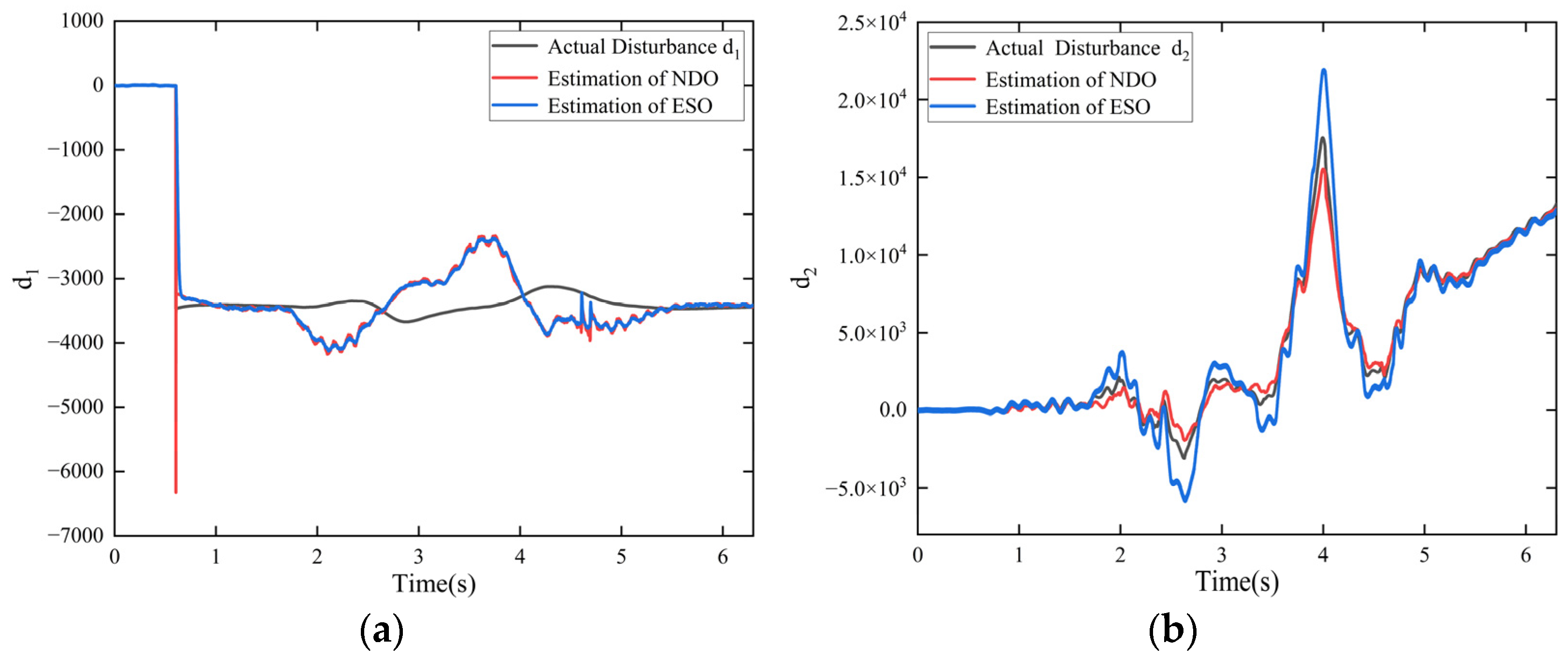
This study utilized MATLAB/Simulink 2021 and Carsim software 2020 for co-simulation to test the performances of the NDO and ESO. In MATLAB/Simulink, the NDO and the ESO were established, while in Carsim, the double lane-change working condition was set, the longitudinal speed of the vehicle was set to 120 km/h, the speed of the crosswind was set to 100 km/h, and the coefficient of the road adhesion was 0.9. The results of the co-simulation are displayed in Figure 2.
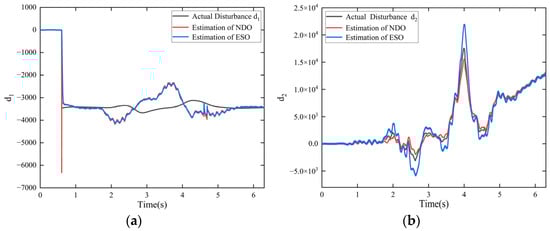
Figure 2.
The estimation results of NDO and ESO: (a) the estimated value of ; (b) the estimated value of .
In the co-simulation, the estimation performance of the disturbance observer was determined by observing the degree of overlap between the actual lateral wind values and the estimated values of the NDO and ESO. At 0.6 s, the vehicle system was subjected to lateral wind disturbance, as shown by the black line in Figure 2, and the estimated values of the NDO and ESO are shown by the red line and blue line in Figure 2, respectively.
Through co-simulation analysis, it was observed that the ESO was superior to the NDO in estimating disturbance in Figure 2a, but the NDO was superior to the ESO in estimating disturbance in Figure 2b. Therefore, to better estimate the external disturbances and unmodeled items, this study utilized a combined approach of the NDO and the ESO to estimate the external disturbances and unmodeled items; the ESO in the union disturbance observer observed the disturbance term , while the NDO observed the disturbance term .
4. Design of Vehicle State Estimator
4.1. Design of Standard Unscented Kalman Filter
The UKF is an improved filtering algorithm developed according to the KF. It does not require the assumption that the state variable’s change is linear, nor does it assume that the relationship between the observation variables and the state variables is linear. The UKF abandons the conventional practice of linearizing nonlinear functions and instead utilizes the KF filtering framework to resolve the problem of nonlinear transmission of covariance and mean, via a one-step prediction equation using the unscented transform (UT). The algorithm approximates the nonlinear functions’ probability density distribution, approximating the state’s posterior probability density using a series of deterministic samples, without the need to linearize the Jacobian matrix. The UKF does not neglect higher-order terms, thus providing higher computational accuracy for statistical quantities of nonlinear distributions, effectively overcoming the poor accuracy of estimation and low stability of the KF and the extended Kalman filter (EKF).
This study adopted a symmetric distribution sampling approach according to the principle of the UT, which is as follows:
Compute Sigma sampling points, where refers to the state’s dimension:
where , denotes the matrix root’s i-th column.
Compute the weight of the Sigma sampling points:
where the subscript represents the mean, represents the covariance, and the superscript represents the sampling point serial number. The argument is a scaling factor used to decrease the overall error of prediction, is used to control the state of the distribution of the Sigma sampling points, is an undetermined argument with no specific limits on its values, typically ensuring that the matrix is a positive semi-definite matrix. The undetermined argument is a nonnegative weight coefficient that can merge the moments of high-order items in the formula, including the effects of high-order items.
The state space model is taken into account to describe the dynamic system as shown in Equations (36) and (37):
where is discrete time, the system’s state at the time is ; is the corresponding state observation signal; is input white noise; is observation noise. Equation (36) represents the state equation, and Equation (37) represents the observation equation. is the state’s matrix of transition, is the driving matrix of noise, and is the observation matrix.
Assuming and is irrelevant white noise disturbance with zero mean and variance matrices and , then , , , . and are uncorrelated; then, , , , , .
Here are the UKF algorithm’s steps:
Use the UT to obtain the Sigma points set and weights:
Calculate the one-step prediction of the Sigma points, :
Compute the system state’s matrix of covariance and one-step prediction, obtained from the predicted values’ weighted sum of the Sigma points. This is the distinction from the traditional KF. The traditional KF requires the state from the previous time step to be input into the state equation and calculates the state prediction only once, while the UKF uses Sigma points set for prediction and calculates their weight average to obtain the system state’s one-step prediction.
Use the UT again to obtain a new set of Sigma points according to the one-step prediction.
Use the predicted Sigma points obtained in step Equation (4) in the observation equation to compute the predicted observation, .
Obtain the predicted covariance and mean of the system by the weighted sum of the observation prediction values of the Sigma points obtained in step Equation (5):
Compute the unscented Kalman gain matrix:
Calculate the system’s state update and covariance update:
This shows that the UKF does not require Taylor series expansion and first approximation up to the -order at the estimation point when dealing with nonlinear filtering. Instead, it uses the UT near the estimation point to obtain a set of Sigma points whose covariance and mean match the raw statistical properties, and then directly utilizes nonlinear mapping of these Sigma points to approximate the state’s probability density function.
To accurately obtain the sideslip angle of the vehicle and other state information [52] while considering external disturbances and unmodeled items affecting the vehicle system, a UKF was designed and is presented in this paper. Its anti-disturbance performance takes the form of Equations (50) and (51), based on Equation (12):
The state equation is:
The observation equation is:
where is the state vector, is the control input vector, is the observation vector, and the random variables , represent process noise and measurement noise, chosen to be mutually independent Gaussian white noise with zero mean; their probability distribution is denoted as:
According to the Equation (12), the UKF is designed as follows:
where the state vector , control input vector , and observation vector are used in the UKF. The variables , in Equation (53) can be obtained by UDO.
4.2. Design of Improved Adaptive Unscented Kalman Filter
In existing research, the process of design of the UKF usually assumes that the noise disturbance is white noise, and sets the matrix of noise covariance as a constant and . However, since the sensor signal contains noise disturbance signals, the covariance matrix of the noise signal may change with the external environment factors. Therefore, the UKF, which is set to a constant noise covariance matrix, has poor practical application results. To improve the noise resistance of the UKF, an improved adaptive noise covariance adjustment strategy (iANCAS) is proposed in this paper [53,54]. This iANCAS algorithm can adaptively adjust and according to the error between the priori measurement and the actual measurement, reducing the estimation errors and the possibility of filter divergence. Additionally, in this paper, the iANCAS approach is associated with the UKF for anti-disturbance performance, to propose an iAUKF for estimating the sideslip angle of the vehicle.
To more accurately approximate the system process noise, the innovation is defined as the error between the priori measurement and the actual measurement, denoted as:
The theoretical covariance matrix of the innovation is obtained through the UKF algorithm, numerically equal to the autocovariance of the predicted output; thus, the innovation’s theoretical covariance is:
The actual innovation’s covariance is obtained using the definition of error covariance, usually set to:
where is the length of the sliding window.
Since existing vehicle dynamics models cannot fully reflect the actual dynamic characteristics of vehicles, modeling errors are always present in the vehicle state estimation process. In addition, the sensors’ performance is affected by external environmental noise during the measurement process, causing the actual covariance of the innovation to deviate from the theoretical covariance. Therefore, the adjustment factor for the noise covariance can be calculated using the deviation between the innovation’s actual covariance and the theoretical covariance.
To avoid the effect of old data on the innovation’s actual covariance and to prevent data overflow, this paper introduces a forgetting factor to adjust the weight of old data [55]. Therefore, Equation (57) can be rewritten as:
where is the threshold for preventing data overflow, is the forgetting factor, and the method for adjusting the forgetting factor is set as:
where , .
Considering that the vehicle’s state is related to working conditions, it is very difficult to achieve simultaneous equilibrium in the error of the steady state of the UKF and the dynamic response by utilizing a constant sliding window length to calculate . Therefore, to adaptively adjust the sliding window value according to different running conditions of the vehicle, this paper proposes the following constraint:
where and are the maximum and minimum values of the sliding window , is the adjustment index measuring the change velocity of the vehicle state, and are the state thresholds used to adjust the sliding window , where and are taken in this case, and the function is used for rounding.
In addition, to avoid the problem of when calculating , and were set as follows [56]:
In addition, in the sliding window adjustment strategy, when , it is considered that the vehicle is in a maneuvering state, where the vehicle state changes rapidly. In this case, if the sliding window is too long, the presence of a large amount of nonmaneuvering innovation data will lead to deviation when calculating the actual covariance of the innovation, which is not conducive to reducing the steady-state error of the noise covariance adaptive adjustment strategy. Therefore, the sliding window’s length should be reduced to reduce the effect of the state changes. When , the vehicle is in a nonmaneuvering steady-state running condition, and the car’s state changes slowly. In this case, if the sliding window is too short, the effects of slow changes of state on the actual covariance of the innovation cannot be considered, so the sliding window’s length should be added to ensure the dynamic response performance of the noise covariance adjustment strategy. When , the cosine expansion method is used to substitute the conventional exponential function adjustment strategy, reducing the computational load of the adaptive algorithm and improving the real-time behavior of the iANCAS.
In addition, as a performance indicator for regulating the sliding window length , needs to accurately reflect the rate of changes in the motion state of the vehicle. When , it is considered that the vehicle state changes rapidly; conversely, when , it is considered that the vehicle’s state change is relatively slow, and the length can be adaptively adjusted based on . Therefore, this paper uses normalized innovation squared (NIS) [57], commonly used in target positioning and tracking, to define the sliding window adjustment index :
By calculating the ratio of and , the noise covariance adjustment factor is obtained [58], expressed as:
Finally, using the calculated noise covariance adjustment factor to adaptively adjust and in the UKF, the modified UKF is represented as:
where is the amplification factor for the adjustment factor, set as in this article.
In addition, to numerically characterize the error of estimation, this paper introduces root mean squared error (RMSE) to measure the estimation error of the iAUKF, expressed as:
where is the vehicle state’s actual value, is the vehicle state’s estimated value, and is the number of estimations of the vehicle state by the iAUKF.
5. Design of Vehicle Stability Control System
In order to effectively control the stability of the vehicle system, this study adopted the direct yaw moment control (DYC) technique [59] to achieve the goal; the control principle is expressed in Figure 3.
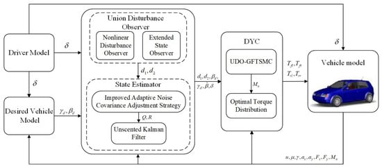
Figure 3.
The control principle of the vehicle stability system.
Since this article does not involve research on vehicle trajectory tracking, the driver model was set up using Carsim to drive the vehicle along a predetermined path. The desired vehicle model was obtained from a linear 2-DOFs model, the ideal yaw rate and ideal sideslip angle were calculated. The union disturbance observer consisted of an NDO and an ESO, which estimated disturbances experienced by the vehicle system. The state estimator was designed using iAUKF to estimate the sideslip angle of the vehicle. The DYC system was designed using the UDO-GFTSMC method to calculate the additional yaw moment required to maintain the lateral stability of the vehicle system. At the same time, the tire force optimization allocation was calculated using a quadratic optimization allocation method. The vehicle model was obtained through Carsim software.
The front wheel steering angle signal was generated by the driver model, the ideal yaw rate and the sideslip angle were generated by the vehicle’s desired model with 2-DOFs. The UDO module consisted of the NDO and the ESO, estimating the vehicle system’s lumped disturbance and . The state estimation module consisted of the UKF method and an iANCAS, where the UKF algorithm estimated the vehicle’s sideslip angle , and the iANCAS optimized the filtering parameters and . UDO can improve the anti-disturbance performance of UKF. The yaw stability control module included the GFTSMC algorithm based on the UDO and the brake force optimization allocation algorithm. The GFTSMC algorithm calculated the additional yaw moment to maintain the vehicle’s stability, and the optimization allocation module optimally allocated the brake forces of the four wheels with the control objective of the optimal slip ratio of the tires, fully utilizing the adhesion conditions of the ground to ensure the vehicle’s stability. All the above modules were established using MATLAB/Simulink, and the vehicle model module was established using Carsim to set the working conditions of the vehicle and external conditions, simulating vehicle motion.
5.1. Design Vehicle Stability System Controller
The vehicle’s yaw stability controller was designed according to the UDO. The motion state of the vehicle is constantly changing during the working process, which requires the stability control system of the vehicle to be real-time. To meet the human driver’s demands for the maneuverability and stability of the vehicle, the sliding mode surface has been designed according to the difference between the yaw rate and the sideslip angle, taking into account external disturbances and unmodeled items affecting the vehicle and GFTSMC.
The tracking error sliding mode surface is designed as:
The definition of the GFTSMC surface is:
where , , , are odd numbers and .
The proposed law of GFTSMC is:
where , can be estimated by the UDO. If the parameters of the control law are chosen to satisfy the following requirement: , , , , then, the GFTSMC law forms a closed-loop system that is finitely time stable, and there exists a settling time , such that for any , the variable of system state .
Proof: Choosing the candidate function of the Lyapunov as:
Taking the derivative of Equation (70):
Thus:
So, it can be obtained that the candidate function of the Lyapunov is negatively definite.
Let ; then, from Equation (68), obtain:
Let ; then, and Equation (73) becomes:
The general solution of the first-order linear differential equation is:
The solution to Equation (74) is:
When , , Equation (75) changes into:
As , , , Equation (76) becomes:
Hence:
where .
The time for the system to converge from any initial state to the balance state is:
By setting , , , , the system can achieve the balance state in finite time .
5.2. Design of Optimal Allocation Controller
This approach optimizes and distributes the brake forces of the braking system for four wheels, taking the optimal slip ratio of tires as the control objective, and fully utilizes the ground adhesion conditions to ensure control of the vehicle motion.
The tire adhesion utilization rate calculation formula is:
where is the longitudinal force of the tire, represent the front left wheel, rear left wheel, front right wheel, and rear right wheel, respectively, and the same notation method is used below; is the adhesion utilization rate of the tire, , and is the vertical load of tire, .
According to Equation (81), for the tire to have good reserve lateral force, the smaller is, the better. So, the objective function can be obtained:
As can be seen from Equation (82), the smaller is, the greater the margin of the stability of the vehicle, and the lower the probability of instability of vehicle. In this study, assignment of additional yaw moments was achieved by adjusting the longitudinal force of the tire. Since it is very difficult to directly control tire lateral force, only the longitudinal force was optimized and controlled, simplifying Equation (82) to:
The controller optimizes the distribution of additional yaw moment, so it is necessary to satisfy the constraint conditions of the additional yaw moment equation:
The tire’s longitudinal force cannot transcend the limit of the ground adhesion condition, and each wheel’s braking force needs to meet:
Equations (83)–(85) were transformed into a quadratic programming standard form for solving, as shown in Equation (86):
6. Simulation
To test the estimation performance of the iAUKF according to the UDO proposed in this article and the control performance of the controller of vehicle stability based on the UDO and the GFTSMC, this study used MATLAB/Simulink and Carsim software for co-simulation testing. The co-simulation parameters are shown in Table 1.

Table 1.
The co-simulation parameters. for anti-disturbance performance testing of the iAUKF.
6.1. The Anti-Disturbance Performance Testing of the iAUKF
To test the anti-disturbance performance of the proposed iAUKF, this study set up double lane-change conditions, the straight-line driving conditions, and the fishhook steering conditions in Carsim. Lateral wind disturbance was also applied to compare the anti-disturbance behavior of the standard UKF and the iAUKF.
6.1.1. Double Lane-Change Test
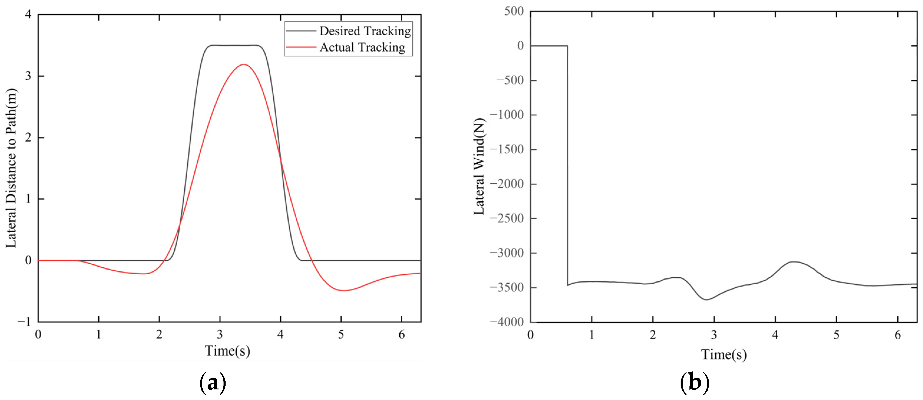
In the double lane-change conditions, the longitudinal velocity was set to 120 km/h, lateral wind to 100 km/h, and the crosswind direction from the left side to the right side of the road where the car was initially located. A driver model was used to track the desired path, as shown in Figure 4a. The lateral wind is displayed in Figure 4b, and the outcomes of co-simulation are shown in Figure 4c,d. Figure 4c shows the estimation results for the sideslip angle for the UKF and iAUKF algorithms under external disturbance. To compare the estimation results, the actual value of the sideslip angle is shown in Figure 4c. Figure 4d shows the estimation error of the UKF and iAUKF algorithms.
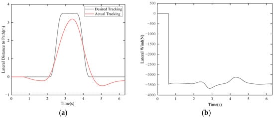
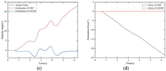
Figure 4.
The results of the double lane-change test: (a) lateral displacement; (b) lateral wind; (c) estimation of vehicle sideslip angle; (d) estimation error of sideslip angle.
At 0.6 s, the vehicle system was subjected to lateral wind disturbance, as shown in Figure 4b. The estimation performance was determined by observing the degree of overlap between the estimated values of UKF and iAUKF, as shown in Figure 4c, and the actual value of the sideslip angle, that is, the degree of overlap between the red, blue, and black lines (the black and blue lines have already overlapped). Meanwhile, the performance of the estimator can also be determined by observing Figure 4d, where the smaller the value, the higher the estimation performance.
It can be observed from Figure 4c,d, that the estimation accuracy of the standard UKF and the iAUKF was the same for the first 0.6 s without lateral wind disturbance, and both accurately estimated the sideslip angle of the vehicle. However, when the lateral wind was imposed from left to right at 0.6 s, the estimation curve of the UKF gradually moved far away from the actual sideslip angle, while that of the iAUKF proposed in this paper remained unchanged; thus, when lateral wind disturbance was imposed, it could still accurately estimate the sideslip angle with high accuracy. In Figure 4d, the maximum estimation error of iAUKF is less than 0.1°.
6.1.2. Straight-Line Driving Test
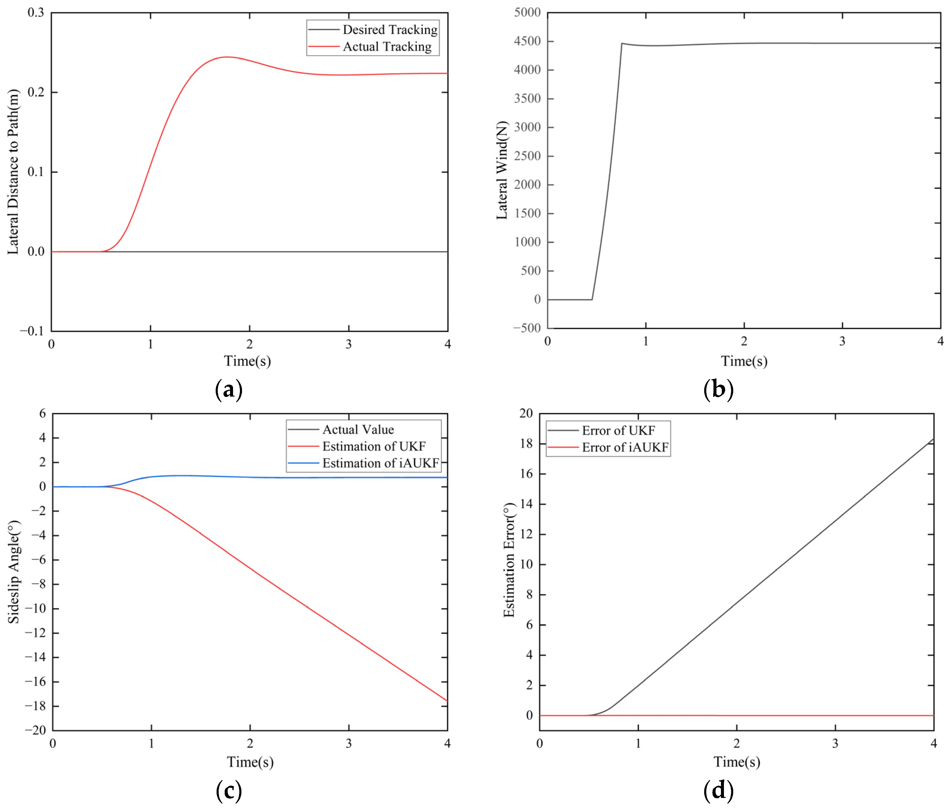
In the straight-line driving conditions, the longitudinal speed was set at 120 km/h, lateral wind at 120 km/h, and the crosswind direction from the right side to the left side of the road at the initial position of the vehicle. A driver model was used to track the straight-line driving path, as shown in Figure 5a. The lateral wind is displayed in Figure 5b, and the results of the co-simulation are displayed in Figure 5c,d. Figure 5c shows the estimation results of the sideslip angle for the UKF and iAUKF algorithms under external disturbance. To compare the estimation results, the actual value of the sideslip angle is shown in Figure 5c. Figure 5d shows the estimation error of the UKF and iAUKF algorithms.
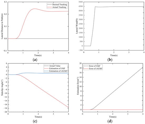
Figure 5.
The results of straight-line driving testing: (a) lateral displacement; (b) lateral wind; (c) estimation value of vehicle sideslip angle; (d) estimation error of sideslip angle.
At 0.6 s, the vehicle system was subjected to lateral wind disturbance, as shown in Figure 5b. The estimation performance was determined by observing the degree of overlap between the estimated values of UKF and iAUKF, as shown in Figure 5c, and the actual value of the sideslip angle, that is, the degree of overlap between the red, blue, and black lines (the black and blue lines have already overlapped). Meanwhile, the performance of the estimator can also be determined by observing Figure 5d, where the smaller the value, the higher the estimation performance.
It can be observed in Figure 5c,d that the co-simulation results were similar to those of the double lane-change simulation. During the first 0.45 s without lateral wind disturbance, both the standard UKF and the iAUKF algorithms correctly estimated the sideslip angle of the vehicle. However, when the vehicle began to experience a lateral wind from right to left at 0.4 s, the estimation accuracy of the standard UKF gradually decreased, and the cumulative error gradually increased over time. However, the estimation curve of the iAUKF proposed in this paper did not change when it experienced lateral wind disturbance, and it was still able to estimate the sideslip angle with high accuracy. In Figure 5d, the maximum estimation error of iAUKF is less than 0.02°.
6.1.3. Test of Fishhook
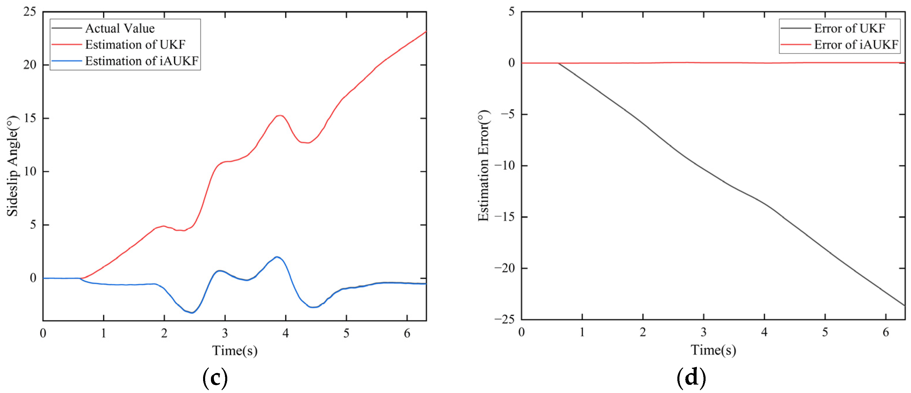
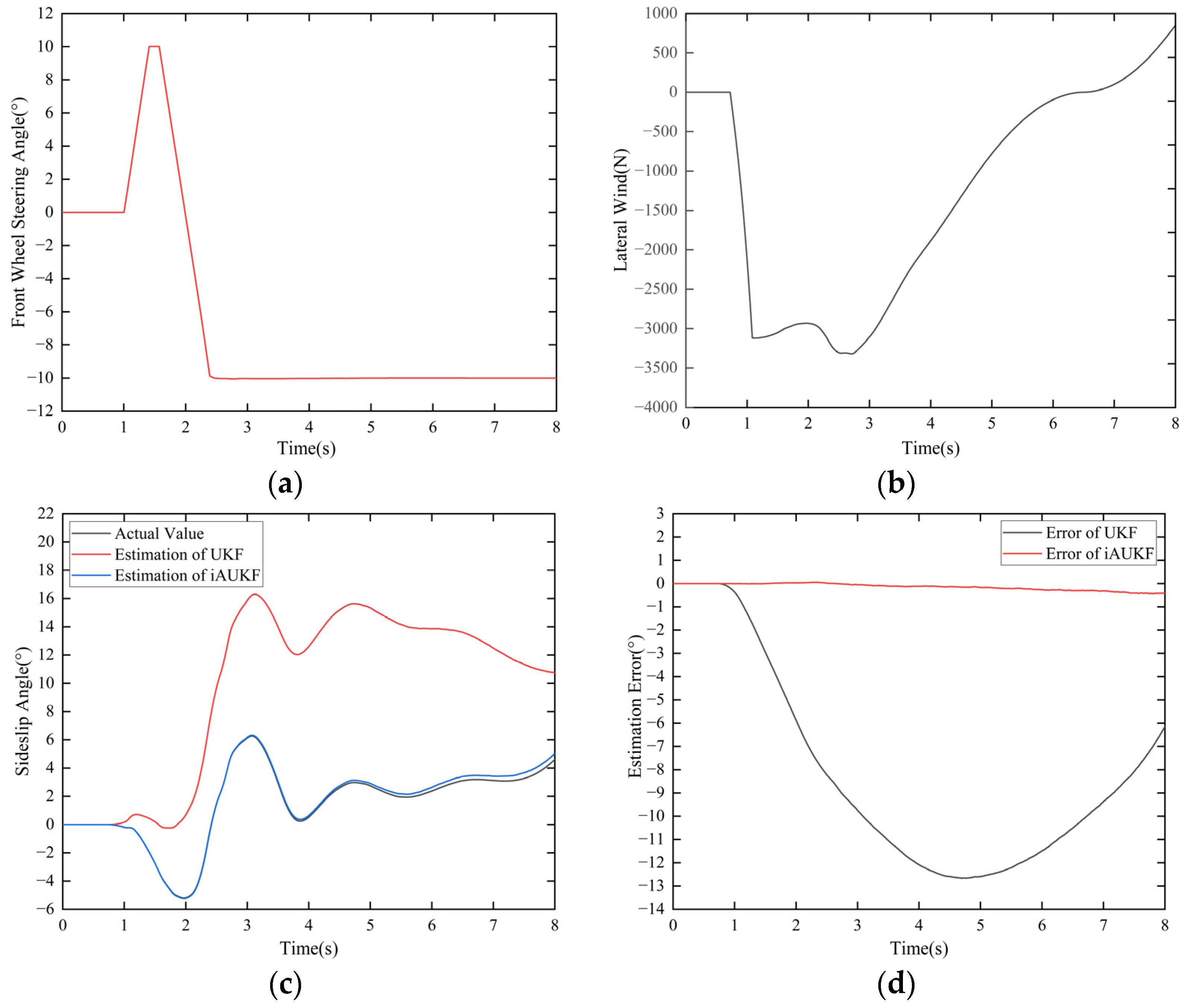
The fishhook maneuver is a typical extreme steering test condition. This study set the longitudinal vehicle speed at 100 km/h, lateral wind at 100 km/h, and the crosswind direction from the left side to the right side of the road at the vehicle’s initial position, a fishhook maneuver simulation was conducted. The change in the steering angle of the front wheel is shown in Figure 6a, and the lateral wind is displayed in Figure 6b. The results of the co-simulation are displayed in Figure 6c,d. Figure 6c shows the estimation results of the sideslip angle for the UKF and iAUKF algorithms under external disturbance. To compare the estimation results, the actual value of the sideslip angle is shown in Figure 6c. Figure 6d shows the estimation error of the UKF and iAUKF algorithms.
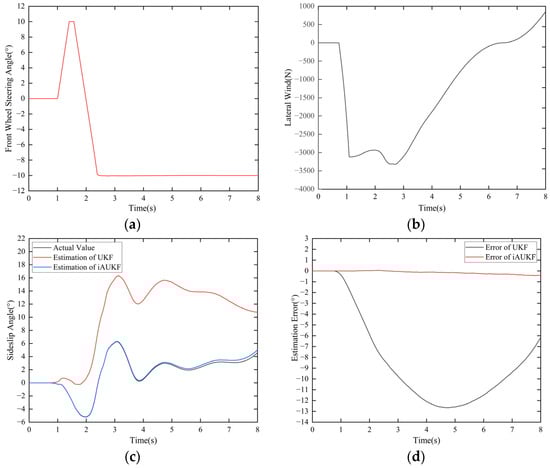
Figure 6.
Fishhook test results: (a) the steering angle of the front wheel; (b) lateral wind; (c) estimation of vehicle sideslip angle; (d) estimation error of sideslip angle.
At 0.6 s, the vehicle system was subjected to lateral wind disturbance, as shown in Figure 6b. The estimation performance was determined by observing the degree of overlap between the estimated values of UKF and iAUKF, as shown in Figure 6c, and the actual value of the sideslip angle, that is, the degree of overlap between the red, blue, and black lines. Meanwhile, the performance of the estimator can also be determined by observing Figure 6d, where the smaller the value, the higher the estimation performance.
Figure 6c,d indicate that the results of the co-simulation were similar to those of the double lane-change simulation and straight-line driving simulation. During the first 0.7 s without lateral wind disturbance, both the standard UKF and the iAUKF accurately estimated the sideslip angle of the vehicle. However, when the vehicle began to experience lateral wind from left to right at 0.7 s, the estimation accuracy of the standard UKF gradually decreased, and the cumulative error gradually increased over time. However, the iAUKF proposed in this paper still accurately estimated the sideslip angle when subjected to lateral wind disturbance. In Figure 6d, the maximum estimation error of iAUKF is less than 0.5°.
From the simulation tests under the three conditions described above, it was concluded that the standard UKF could not correctly estimate the vehicle’s sideslip angle when external lateral wind disturbance was imposed, and the estimation error gradually accumulated over time. However, the iAUKF proposed in this article correctly estimated the sideslip angle and resisted external disturbances.
6.2. The Anti-Noise Performance Test of the iAUKF
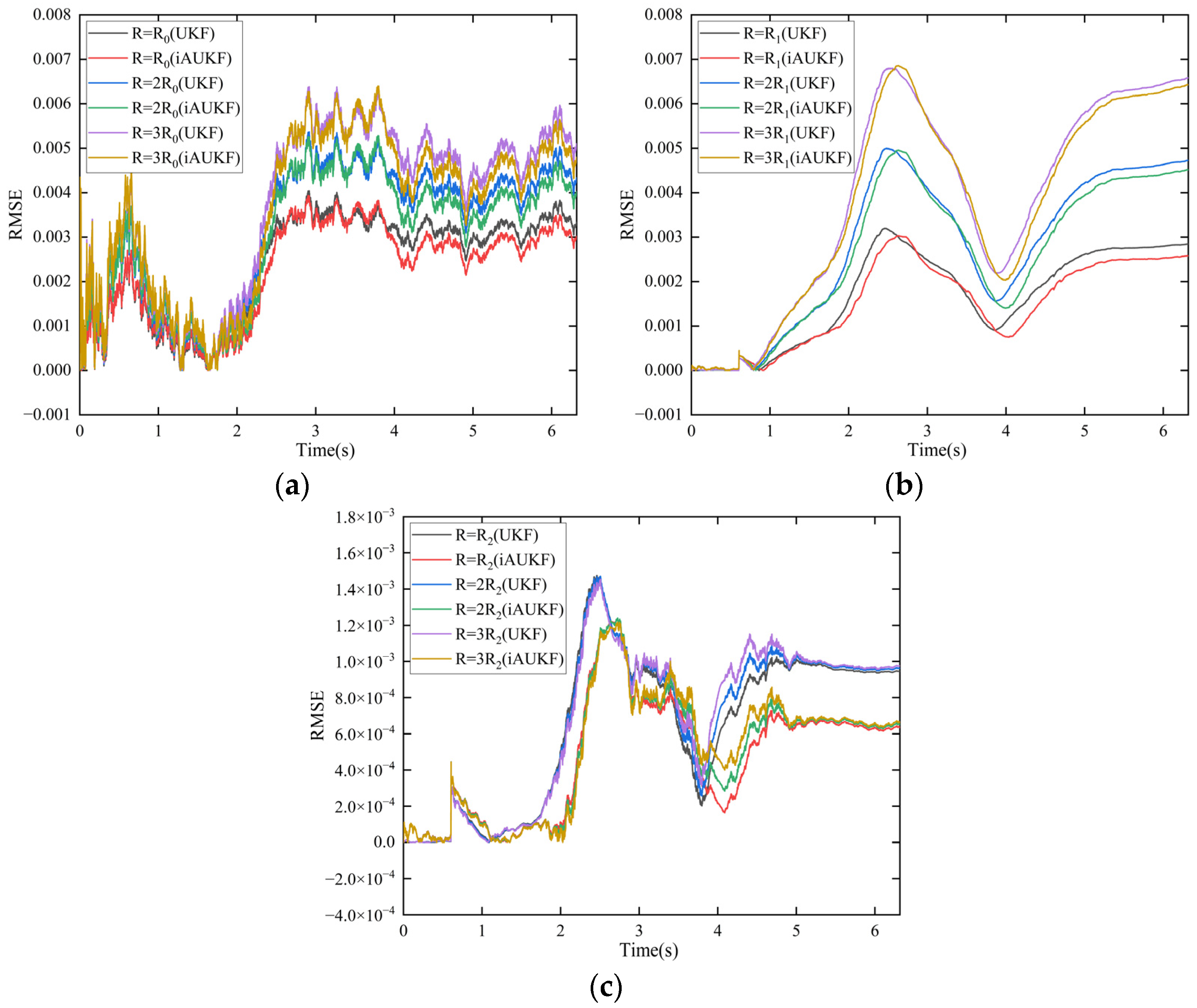
To test the anti-noise performance of the proposed iAUKF, this research selected the double lane-change condition for testing, imposed noise disturbance signals on the yaw rate sensor, the sensor of the front wheel steering angle, and longitudinal speed sensor, respectively, and compared the anti-noise behavior of the standard UKF and the iAUKF under different levels of disturbance strength. The results of the co-simulation are displayed in Figure 7. Figure 7 shows the estimation performances of UKF and iAUKF under different intensities of noise disturbance, for the yaw rate sensor, front wheel angle sensor, and longitudinal speed sensor.
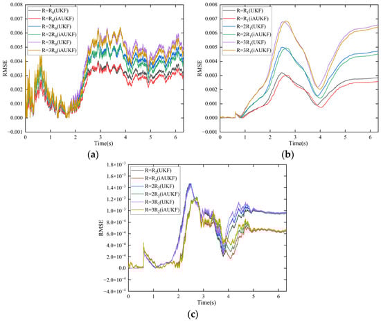
Figure 7.
The results of anti-noise performance testing of the iAUKF: (a) the yaw rate sensor is disturbed by noise; (b) the steering angle of the front wheel sensor is disturbed by noise; (c) the longitudinal velocity sensor is disturbed by noise.
Throughout the simulation process, the sensor was constantly affected by noise disturbance, and from 0.6 s to end, it was also affected by lateral wind disturbance. The anti-noise performance of iAUKF was assessed by observing the curve in Figure 7. The smaller the value, the stronger was the anti-noise performance. Noises of different intensities were applied separately and the anti-noise performance of iAUKF was observed.
Figure 7a indicates that when the noise disturbance was imposed on the yaw rate sensor, the overall RMSE value of the iAUKF was lower than that of the standard UKF under the same disturbance signal strength level, indicating that the estimation accuracy of the iAUKF was higher than that of the standard UKF. At the same time, as the disturbance signal strength level increased, the estimation accuracy of both UKFs decreased, but the estimation accuracy of the iAUKF was still superior to that of the standard UKF. The results of the co-simulation of the steering angle of the front wheel sensor and longitudinal speed sensor under noise disturbance were similar to those for the yaw rate sensor under noise disturbance.
By comparing the estimation errors of the UKF and the iAUKF when different levels of disturbance signals were imposed on the sensors of the vehicle system, it was found that the iAUKF proposed in this article was able to adjust the filtering parameters adaptively based on external disturbances, thus resisting the problem of increased state estimation error caused by sensor noise.
6.3. The Test of Vehicle Stability Controller Performance
To test the behavior of the vehicle stability controller according to the UDO and GFTSMC, this paper describes tests with double lane-changing conditions, sine steering conditions, and fishhook steering conditions in Carsim. Lateral wind disturbances were also set up to test the performance of the vehicle stability controller proposed in this article.
6.3.1. Tight Double-Lane Change Test
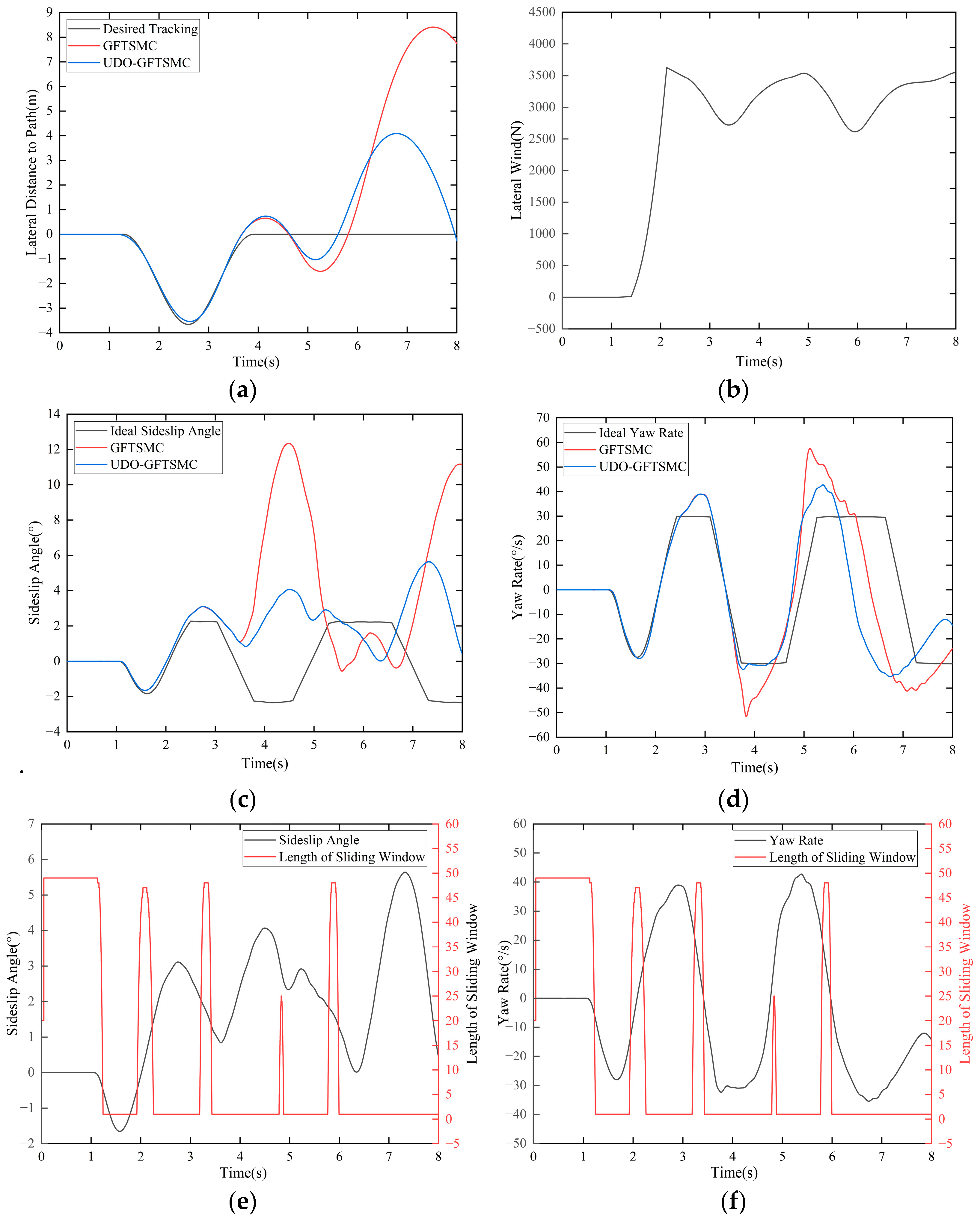
In this test, the longitudinal velocity was set at 52 km/h, lateral wind at 120 km/h, and the wind direction from the right side to the left side of the road where the vehicle was initially located. A driver model was used to track the desired path, as shown in Figure 8a. The lateral wind is displayed in Figure 8b, and the results of the co-simulation are shown in Figure 8c–f. Figure 8c,d show the control effects of the sideslip angle and yaw rate with GFTSMC and UDO-GFTSMC under lateral wind disturbance, respectively; Figure 8e,f show the variation trends for sliding window length in iAUKF.
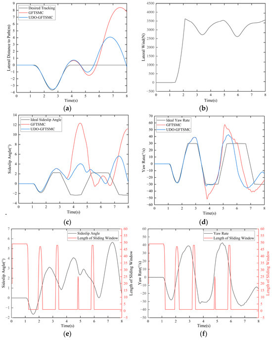
Figure 8.
The results of the tight double lane-change test: (a) lateral displacement; (b) lateral wind; (c) change of sideslip angle with the controllers; (d) change of yaw rate with the controllers; (e) changes in the sliding window length and sideslip angle; (f) changes in the sliding window length and yaw rate.
Through Figure 8a,c,d, the control performance of the vehicle stability controller were determined. The higher the degree of overlap between the variables and the desired values under the designed controller control, the better was its performance. Figure 8b shows the starting time and numerical values of lateral wind disturbance experienced by the vehicle system. Figure 8e,f show the trend in iAUKF sliding window values as the vehicle state changed. The more severe the vehicle state change, the smaller the sliding window value.
As shown in Figure 8a, in this study, under lateral wind disturbance, the lateral displacement of the stability control system without considering external disturbances was more than that of the stability control system considering external disturbances, demonstrating that the system of control proposed in this article can effectively ensure the vehicle’s lateral stability. As displayed in Figure 8c,d, the control system of stability considering external disturbances was able to effectively ensure the vehicle’s lateral stability, and the changes in the yaw rate and the sideslip angle were both smaller than those of the controller without considering external disturbances. In addition, under the double lane-change condition, the vehicle state changed dramatically and adapted to the vehicle system state. When the vehicle was in a maneuvering state, had a small value, as shown in Figure 8e,f, from 1.2 s to 8 s. When the vehicle was in a nonmaneuvering state, had a large value. This indicates that the iANCAS proposed in this paper was able to effectively adjust according to changes in vehicle state.
6.3.2. Sine Steering Test
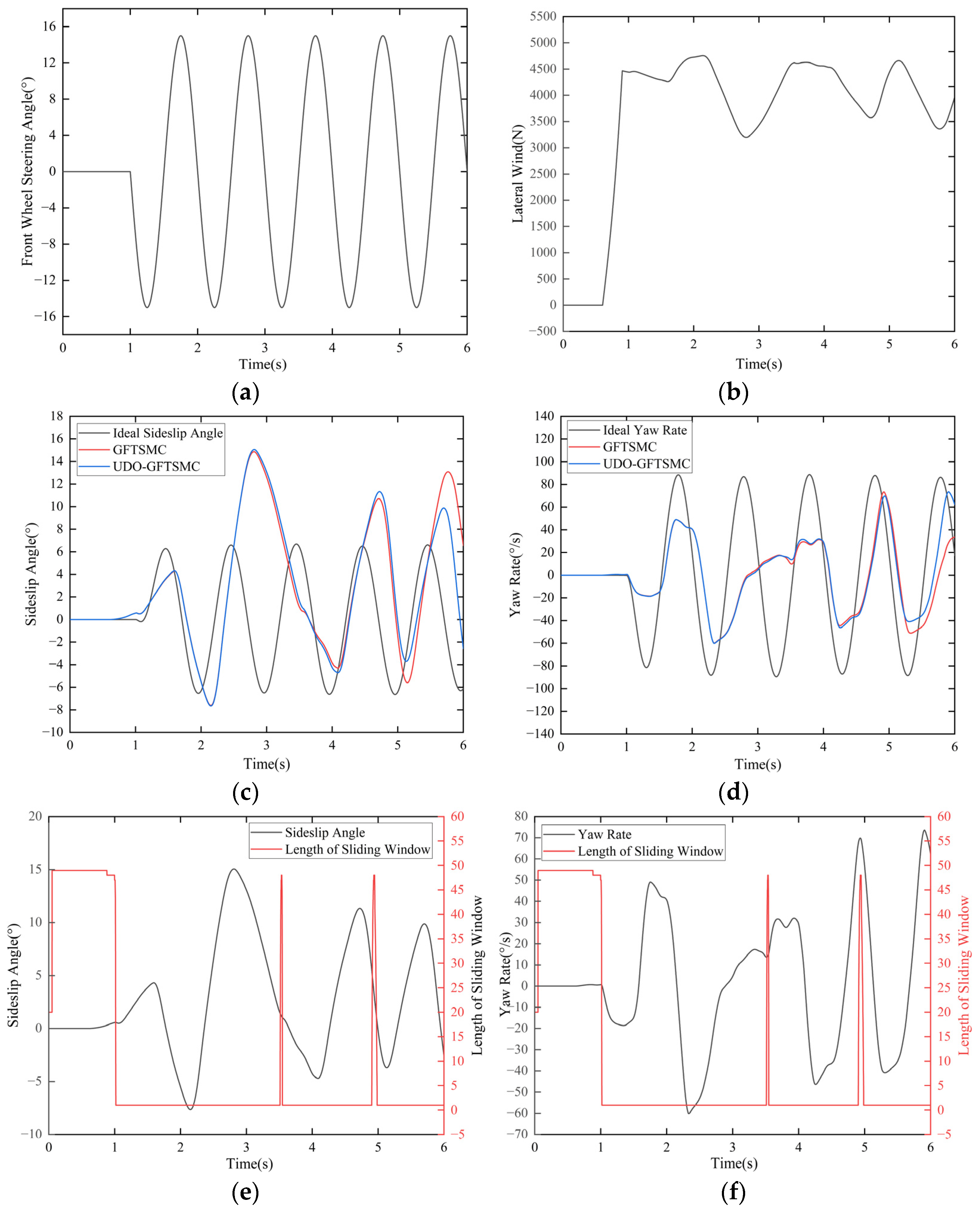
Under sine steering conditions, the longitudinal velocity was set at 120 km/h, and lateral wind at 120 km/h, with the crosswind direction from the right side to the left side of the road at the vehicle’s initial position. The change in the steering angle of the front wheel is shown in Figure 9a, and the lateral wind is displayed in Figure 9b. The results of the co-simulation are displayed in Figure 9c–f. Figure 9c,d show the control effects of the sideslip angle and yaw rate with GFTSMC and UDO-GFTSMC under lateral wind disturbance, respectively. Figure 9e,f show the variation trends in sliding window length in iAUKF.
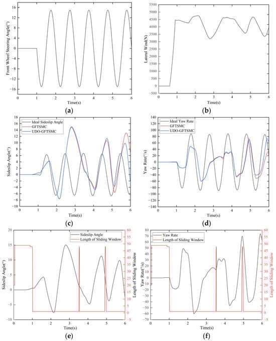
Figure 9.
Results of the sine steering test: (a) steering angle of the front wheel; (b) lateral wind; (c) change of sideslip angle with the controllers; (d) change of yaw rate with the controllers; (e) changes in the sliding window length and sideslip angle; (f) changes in the sliding window length and yaw rate.
From Figure 9a, the running conditions of the vehicle system can be determined. Figure 9b shows the starting time and numerical values of lateral wind disturbance experienced by the vehicle system. Through Figure 9c,d, the control performance of the vehicle stability controller can be determined; the higher the degree of overlap between the variables and the desired values under the designed controller control, the better its performance. Figure 9e,f show the trend in iAUKF sliding window values as the vehicle state changed. The more severe the change in the vehicle state, the smaller was the value of the sliding window.
Figure 9c,d reveal that the results of co-simulation were similar to those of the double lane-change simulation. The behavior of the proposed control system considering external disturbances was better than that of the control system without considering external disturbances. At the same time, due to the vehicle system’s maneuvering state under sine steering conditions, was adaptively adjusted based on the vehicle system state, and the value was small, as displayed in Figure 9e,f, from 1 s to 6 s, indicating that the iANCAS proposed in the article was able to adaptively adjust according to changes in vehicle state.
6.3.3. Fishhook Test
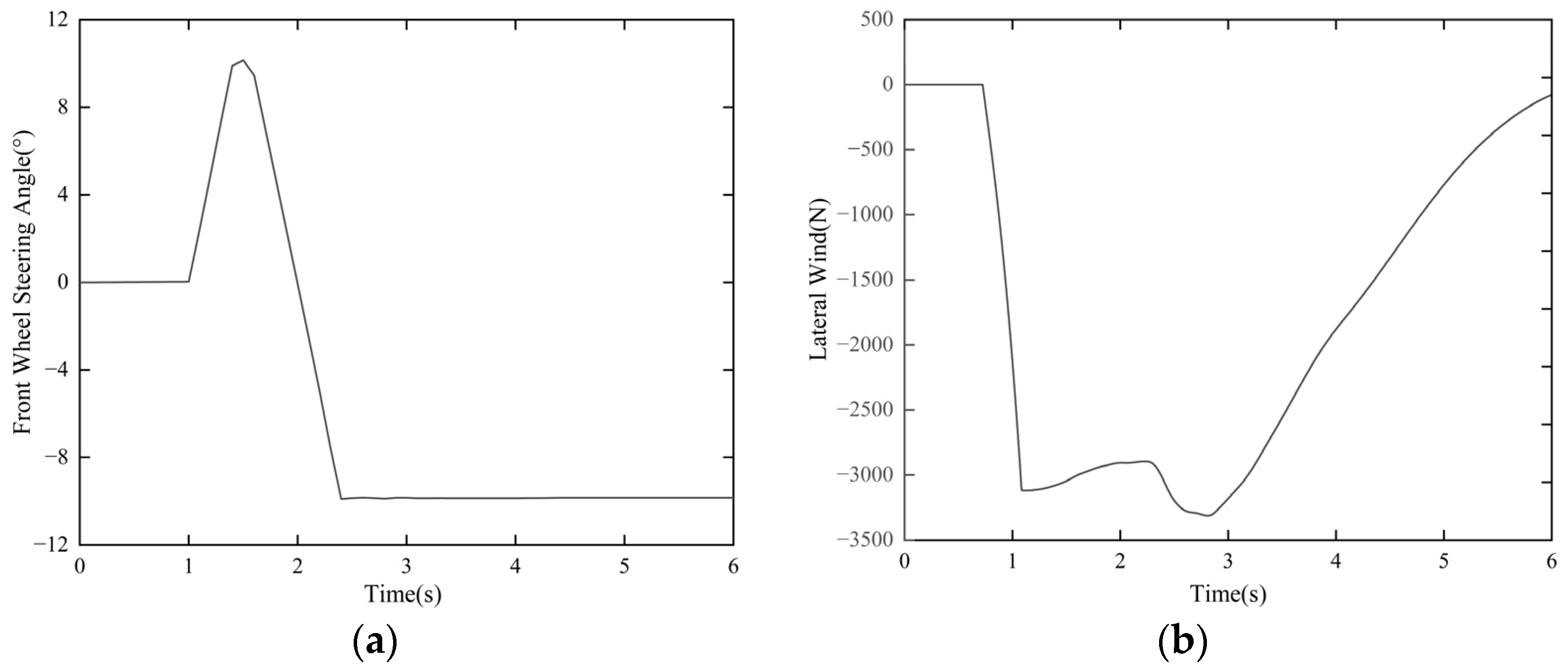
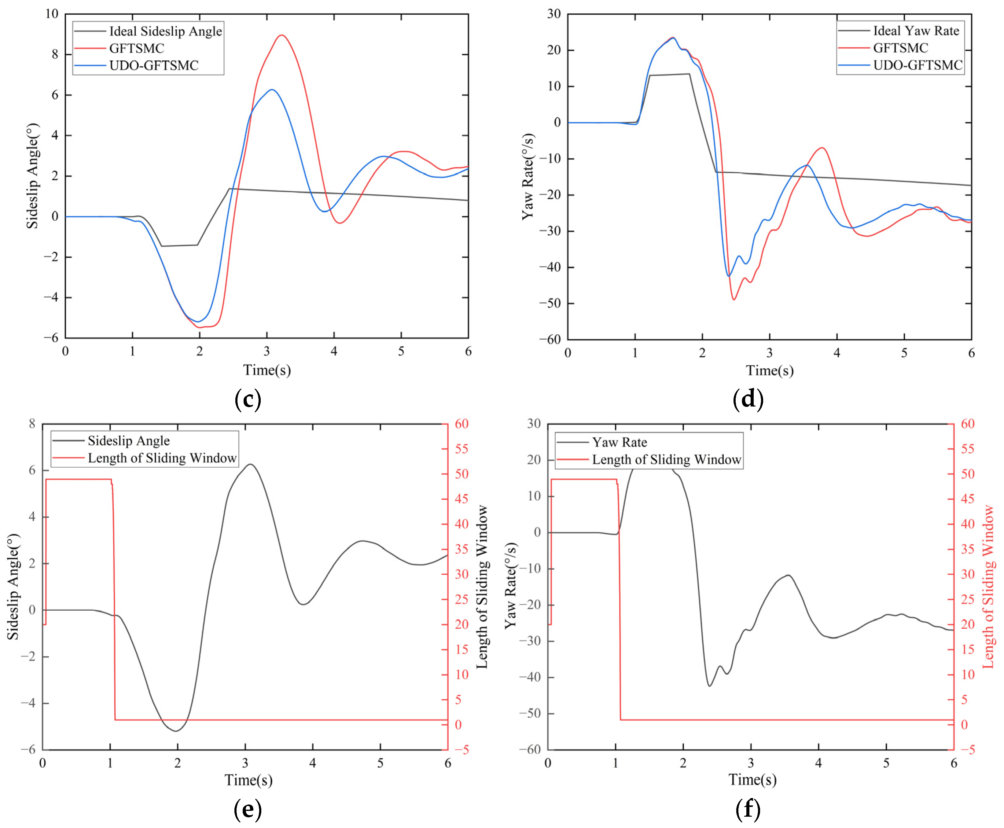
The fishhook maneuver simulation was conducted with the following settings: longitudinal vehicle speed 120 km/h, lateral wind 100 km/h, and crosswind direction from the left side to the right side of the road at the vehicle’s initial position. The change in the steering angle of the front wheel is shown in Figure 10a, and the lateral wind is displayed in Figure 10b. The outcomes of the co-simulation are shown in Figure 10c–f. Figure 10c,d show the control effects of the sideslip angle and yaw rate for GFTSMC and UDO-GFTSMC under lateral wind disturbance, respectively; Figure 10e,f show the variation trends in sliding window length for iAUKF.
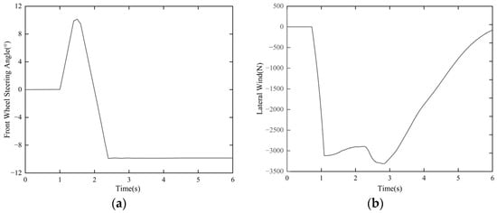
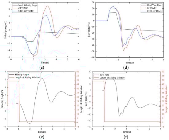
Figure 10.
The fishhook test results: (a) steering angle of the front wheel; (b) lateral wind; (c) change of sideslip angle with the controllers; (d) change of yaw rate with the controllers; (e) changes in the sliding window length and sideslip angle; (f) changes in the sliding window length and yaw rate.
From Figure 10a, the running conditions of the vehicle system can be determined. Figure 10b shows the starting time and numerical values of lateral wind disturbance experienced by the vehicle system. Through Figure 10c,d, the control performance of the vehicle stability controller can be determined. The higher the degree of overlap between the variables and the desired values under the designed controller control, the better was its performance. Figure 10e,f show the trend in iAUKF sliding window values as the vehicle state changed. The more severe the change in vehicle state, the smaller was the sliding window value.
Figure 10c,d, show that the results of the co-simulation were similar to those of the double lane-change simulation and the sine steering simulation. The behavior of the proposed control system considering external disturbances was better than that of the control system without considering external disturbances. Under the fishhook conditions, the self-adaptive adjustment was made as the vehicle system state changed, indicating that the iANCAS proposed in this article adjusted well to changes in vehicle state.
From the above results of the three co-simulations, it can be concluded that the GFTSMC based on a UDO, as proposed in this article, can effectively control vehicle stability, effectively resist the decline in control accuracy caused by external disturbances, and enhance the control system’s robustness.
7. Conclusions
To enhance the estimation behavior and ability of the anti-disturbance features of the UKF and the control performance and robustness of the vehicle stability controller, this article considers the effects of external disturbances on the estimation behavior of the UKF and the stability control of the vehicle. A UDO was designed based on the NDO and the ESO, which optimizes the parameters of the UKF by combining with the iANCAS. The vehicle stability controller, designed according to the UDO and GFTSMC, controls the vehicle’s stability. Finally, through co-simulation analysis, the following conclusions can be stated:
By designing the UDO based on the NDO and the ESO, it was possible to effectively observe the external disturbances of the vehicle system, as well as unmodeled items during the modeling process of the vehicle system, providing a more realistic and accurate vehicle dynamics model for the UKF and the vehicle stability controller.
An iAUKF considering external disturbances is proposed, which not only enables adaptive updating and adjustment of filtering parameters but also improves the anti-disturbance capability of the UKF, achieving accurate and real-time estimation of the state of the vehicle system under various running conditions, offering a precise determination of vehicle state for the vehicle stability control system.
Based on the UDO and GFTSMC, the vehicle stability controller was designed, which not only improved the vehicle stability control accuracy but also enhanced the robustness of the vehicle stability controller, greatly improving the vehicle’s driving safety and satisfying the relevant safety requirements.
Of course, there are still limitations to this study. Firstly, in the process of estimating the sideslip angle, the yaw rate, the front wheel steering angle, and the tire lateral force are required. However, the estimation of yaw rate and front wheel steering angle sensor failure were not considered, and the estimation performance under sensor failure conditions cannot be guaranteed. Secondly, tire lateral force information requires the establishment of a tire model, and tire model parameters need to be calibrated through experiments, so the process of obtaining tire model parameters is cumbersome. Therefore, in order to address the above limitations, we will design improved state estimation strategies and methods for sensor fault conditions, while exploring new methods to reduce the workload of obtaining necessary information.
Author Contributions
Conceptualization, J.L. (Jing Li) and B.F.; methodology, B.F.; software, B.F. and L.Z.; validation, B.F.; formal analysis, B.F. and J.L. (Jing Li); investigation, B.F.; writing—original draft preparation, B.F.; writing—review and editing, J.L. (Jin Luo). All authors have read and agreed to the published version of the manuscript.
Funding
This research received no external funding.
Data Availability Statement
The data that support the findings of this study are available from the corresponding author upon reasonable request.
Conflicts of Interest
The authors declare no conflicts of interest.
References
- Wang, Z.; Dong, M.; Gu, L.; Rath, J.; Qin, Y.; Bai, B. Influence of road excitation and steering wheel input on vehicle system dynamic responses. Appl. Sci. 2017, 7, 570. [Google Scholar] [CrossRef]
- Indu, K.; Kumar, A. Electric vehicle control and driving safety systems: A review. IETE J. Res. 2020, 69, 482–498. [Google Scholar] [CrossRef]
- Men, J.; Wu, B.; Chen, J.; Zhang, Z. Comparisons of vehicle stability controls based on 4WS, Brake, Brake-FAS and IMC techniques. Veh. Syst. Dyn. 2012, 50, 1053–1084. [Google Scholar] [CrossRef]
- Zhao, Y.N.; Wang, Z.H.; Sun, M.M.; Liang, B.; Shao, L.B.; Tang, Y. Research on vehicle driving stability based on dynamics co-simulation. In Proceedings of the Journal of Physics: Conference Series, Guilin, China, 15–17 January 2021; Volume 1820. [Google Scholar]
- Acosta, L.C.; Domenico, B.; Stefano, D.G. Nonlinear observer-based adaptive control of ground vehicles with uncertainty estimation. J. Frankl. Inst. 2023, 360, 14175–14189. [Google Scholar] [CrossRef]
- Meetei, L.V.; Das, D.K. Enhanced nonlinear disturbance observer based sliding mode control design for a fully active suspension system. Int. J. Dynam. Control 2020, 9, 971–984. [Google Scholar] [CrossRef]
- Wang, H.; Xu, S.; Zhou, D.; Wang, X.; Liu, X. Vehicle mass-centroid sideslip angle estimation based on extension fusion of fuzzy sliding-mode observer and sensor signal integral. Trans. Beijing Inst. Technol. (Chin. Ed.) 2022, 42, 713–722. [Google Scholar] [CrossRef]
- Shao, K.; Zheng, J.; Deng, B.; Huang, K.; Zhao, H. Active steering control for vehicle rollover risk reduction based on slip angle estimation. IET Cyber-Syst. Robot. 2020, 2, 132–139. [Google Scholar] [CrossRef]
- Yan, Y.; Zhang, H.; Sun, J.; Wang, Y. Adaptive fuzzy observer-based mismatched faults and disturbance design for singular stochastic T-S fuzzy switched systems. J. Vib. Control 2022, 29, 2265–2276. [Google Scholar] [CrossRef]
- Sun, Y.; Gao, C.; Wu, L.B.; Yang, Y.H. Fuzzy observer-based command filtered tracking control for uncertain strict-feedback nonlinear systems with sensor faults and event-triggered technology. Nonlinear Dyn. 2023, 111, 8329–8345. [Google Scholar] [CrossRef]
- Xu, X.; Xia, X.; Zheng, M.; Zhang, N.; Chen, Y. Vibration control of electromagnetic damper system based on state observer and disturbance compensation. J. Vib. Eng. Technol. 2022, 10, 3133–3146. [Google Scholar] [CrossRef]
- Wang, H.; Chang, L.; Tian, Y. Extended state observer-based backstepping fast terminal sliding mode control for active suspension vibration. J. Vib. Control 2020, 27, 2303–2318. [Google Scholar] [CrossRef]
- Allous, M.; Mrabet, K.; Zanzouri, N. Fault tolerant control of eps system with sensor fault. J. Circuits Syst. Comput. 2018, 28, 1950116. [Google Scholar] [CrossRef]
- Yang, B.; Liu, M.; Kim, H.; Cui, X. Luenberger-sliding mode observer based fuzzy double loop integral sliding mode controller for electronic throttle valve. J. Process Control 2018, 61, 36–46. [Google Scholar] [CrossRef]
- Qi, G.; Fan, X.; Li, H. A comparative study of the recursive least squares and fuzzy logic estimation methods for the measurement of road adhesion coefficient. Aust. J. Mech. Eng. 2021, 21, 1230–1246. [Google Scholar] [CrossRef]
- Kim, M.; Choi, G.; Hong, M. Vehicle mass estimation algorithm using recursive least squares method with forgetting and lowpass filter. Trans. Korean Soc. Automot. 2019, 27, 833–838. [Google Scholar] [CrossRef]
- Liu, Y.; Cui, D. Vehicle dynamics prediction via adaptive robust unscented particle filter. Adv. Mech. Eng. 2023, 15, 16878132231170766. [Google Scholar] [CrossRef]
- Liu, Y.; Cui, D.; Peng, W. Vehicle state and parameter estimation based on adaptive robust unscented particle filter. J. Vibroeng. 2022, 25, 392–408. [Google Scholar] [CrossRef]
- Zha, Y.; Liu, X.; Ma, F.; Liu, C.C. Vehicle state estimation based on extended Kalman filter and radial basis function neural networks. Int. J. Distrib. Sens. Netw. 2022, 18, 15501329221102730. [Google Scholar] [CrossRef]
- Manriquez-Padilla, C.G.; Cueva-Perez, I.; Dominguez-Gonzalez, A.; Elvira-Ortiz, D.A.; Perez-Cruz, A.; Saucedo-Dorantes, J.J. State of charge estimation model based on genetic algorithms and multivariate linear regression with applications in electric vehicles. Sensors 2023, 23, 2924. [Google Scholar] [CrossRef]
- Feng, S.; Li, X.; Zhang, S.; Jian, Z.; Duan, H.; Wang, Z. A review: State estimation based on hybrid models of Kalman filter and neural network. Syst. Sci. Control Eng. 2023, 11, 2173682. [Google Scholar] [CrossRef]
- Ruggaber, J.; Brembeck, J. A novel Kalman filter design and analysis method considering observability and dominance properties of measurands applied to vehicle state estimation. Sensors 2021, 21, 4750. [Google Scholar] [CrossRef]
- Wang, P.; Pang, H.; Xu, Z.; Jin, J. On co-estimation and validation of vehicle driving states by a UKF-based approach. Mech. Sci. 2021, 12, 19–30. [Google Scholar] [CrossRef]
- Zhong, S.; Zhao, Y.; Ge, L.; Shan, Z.; Ma, F. Vehicle state and bias estimation based on unscented Kalman filter with vehicle hybrid kinematics and dynamics models. Automot. Innov. 2023, 6, 571–585. [Google Scholar] [CrossRef]
- Zhang, F.; Feng, J.; Qi, D.; Liu, Y.; Shao, W.; Qi, J.; Lin, Y. Joint Estimation of vehicle state and parameter based on maximum correntropy adaptive unscented Kalman filter. Int. J. Automot. Technol. 2023, 24, 1553–1566. [Google Scholar] [CrossRef]
- Wang, Z.; Xue, X.; Wang, Y. State parameter estimation of distributed drive electric vehicle based on adaptive unscented Kalman filter. Trans. Beijing Inst. Technol. (Chin. Ed.) 2018, 38, 698–702. [Google Scholar] [CrossRef]
- Wan, W.; Feng, J.; Song, B.; Li, X. Huber-based robust unscented Kalman filter distributed drive electric vehicle state observation. Energies 2021, 14, 750. [Google Scholar] [CrossRef]
- Wang, L.; Pang, H.; Wang, P.; Liu, M.; Hu, C. A yaw stability-guaranteed hierarchical coordination control strategy for four-wheel drive electric vehicles using an unscented Kalman filter. J. Frankl. Inst. 2023, 360, 9663–9688. [Google Scholar] [CrossRef]
- Liu, Y.; Dou, C.; Shen, F.; Sun, Q. Vehicle state estimation based on unscented Kalman filtering and a genetic-particle swarm algorithm. J. Inst. Eng. Ser. C 2021, 102, 447–469. [Google Scholar] [CrossRef]
- Liu, Y.; Cui, D. Estimation algorithm for vehicle state estimation using ant lion optimization algorithm. Adv. Mech. Eng. 2022, 14, 16878132221085839. [Google Scholar] [CrossRef]
- Novi, T.; Capitani, R.; Annicchiarico, C. An integrated artificial neural network–unscented Kalman filter vehicle sideslip angle estimation based on inertial measurement unit measurements. J. Automob. Eng. 2019, 233, 1864–1878. [Google Scholar] [CrossRef]
- Zhang, C.; Feng, Y.; Wang, J.; Gao, P.; Qin, P. Vehicle sideslip angle estimation based on radial basis neural network and unscented Kalman filter algorithm. Actuators 2023, 12, 371. [Google Scholar] [CrossRef]
- Swain, S.K.; Rath, J.J.; Veluvolu, K.C. Neural network based robust lateral control for an autonomous vehicle. Electronics 2021, 10, 510. [Google Scholar] [CrossRef]
- Reichhartinger, M.; Falkensteiner, R.; Horn, M. Robust estimation of forces for suspension system control. IFAC-PapersOnLine 2018, 51, 328–333. [Google Scholar] [CrossRef]
- Minh, C.H.; Thien, D.T.; Kwan, K.A. Adaptive sliding mode control based nonlinear disturbance observer for active suspension with pneumatic spring. J. Sound Vib. 2021, 509, 116241. [Google Scholar] [CrossRef]
- Choi, M.; Choi, K.; Cho, M.; Lee, M.; Kim, K.S. Chattering reduction of sliding mode control via nonlinear disturbance observer for anti-lock braking system and verification with carsim simulation. Int. J. Automot. Technol. 2023, 24, 1141–1149. [Google Scholar] [CrossRef]
- Zhang, X.; Wang, X.; Gong, X.; Huang, J.; Huang, D.; Wang, P. Segmented identification method of tire-road friction coefficient for intelligent vehicles. Automot. Eng. 2023, 45, 1923–1932. [Google Scholar] [CrossRef]
- Meng, Q.; Li, B.; Hu, C. Nonlinear vehicle active suspension system control method based on the extended high gain observer. Int. J. Veh. Des. 2023, 91, 303–321. [Google Scholar] [CrossRef]
- Shi, Q.; Xu, Z.; Wei, Y.; Wang, M.; Zheng, X.; He, L. Electric motor steer-by-wire angle tracking by proportional differential sliding mode controller with disturbance observer. J. Automob. Eng. 2022, 237, 2696–2707. [Google Scholar] [CrossRef]
- Zhang, J.; Zhou, S.; Zhao, J.; Shi, T. Wheel slip rate tracking control based on nonlinear disturbance observer. J. Huazhong Univ. Sci. Technol. Nat. Sci. Ed. 2020, 48, 44–49. [Google Scholar] [CrossRef]
- Sawant, J.; Chaskar, U. A non-linear disturbance observer-based cooperative adaptive cruise control for real traffic scenarios. Proc. Inst. Mech. Eng. Part D 2022, 236, 2057–2069. [Google Scholar] [CrossRef]
- Xu, H.; Zhao, Y.; Wang, Q.; Lin, F.; Pi, W. Decoupling control of active suspension and four-wheel steering based on Backstepping-ADRC with mechanical elastic wheel. Proc. Inst. Mech. Eng. Part D 2022, 236, 2356–2373. [Google Scholar] [CrossRef]
- Kang, N.; Han, Y.; Wang, B.; Guan, T.; Feng, W. Linear quadratic regulator based on extended state observer–based active disturbance rejection control of autonomous vehicle path following control. Proc. Inst. Mech. Eng. Part I 2023, 237, 102–120. [Google Scholar] [CrossRef]
- Wang, J.; Cai, Y.; Chen, L.; Wang, S.; Shi, D. Coordinated control of hybrid electric vehicle based on extended state observer estimation. J. Zhejiang Univ. Eng. Sci. 2021, 55, 1225–1233. [Google Scholar] [CrossRef]
- Li, B.; Du, H.; Li, W. Trajectory control for autonomous electric vehicles with in-wheel motors based on a dynamics model approach. IET Intell. Transp. Syst. 2016, 10, 318–330. [Google Scholar] [CrossRef]
- Huang, X.; Zha, Y.; Lv, X.; Quan, X. Torque fault-tolerant hierarchical control of 4wid electric vehicles based on improved MPC and SMC. IEEE Access 2023, 11, 132718–132734. [Google Scholar] [CrossRef]
- Denny, D.C.; Kumar, R.P. An adaptive continuous nonsingular fast terminal SMC for permanent magnet synchronous motor fed electric vehicle. Eur. J. Control 2024, 75, 1–13. [Google Scholar] [CrossRef]
- Zhang, Y.; Liu, K.; Gao, F.; Zhao, F. Research on path planning and path tracking control of autonomous vehicles based on improved APF and SMC. Sensors 2023, 23, 7918. [Google Scholar] [CrossRef] [PubMed]
- Dai, P.; Katupitiya, J. Force control for path following of a 4WS4WD vehicle by the integration of PSO and SMC. Vehicle Syst. Dyn. 2018, 56, 1682–1716. [Google Scholar] [CrossRef]
- Li, S.; Yang, J.; Chen, W.; Chen, X. Disturbance Observer-Based Control: Methods and Applications, 1st ed.; The CRC Press: Boca Raton, FL, USA, 2014; pp. 43–44. [Google Scholar]
- Yu, S.; Wang, J.; Wang, Y.; Chen, H. Disturbance observer based control for four wheel steering vehicles with model reference. IEEE-CAA J. Autom. 2018, 5, 1121–1127. [Google Scholar] [CrossRef]
- Tian, Y.; Zhang, Y.; Wang, X.; Chen, H. Estimation of side-slip angle of electric vehicle based on square-root unscented Kalman filter algorithm. J. Jilin Univ. Eng. Technol. Ed. 2018, 48, 845–852. [Google Scholar] [CrossRef]
- Zhang, Z.; Jiang, L.; Zhang, L.; Huang, C. State-of-charge estimation of lithium-ion battery pack by using an adaptive extended Kalman filter for electric vehicles. J. Energy Storage 2021, 37, 102457. [Google Scholar] [CrossRef]
- Pang, H.; Wang, P.; Wang, M.; Hu, C. On accurate estimation of vehicle lateral states based on an improved adaptive unscented Kalman filter. Proc. Inst. Mech. Eng. Part D 2022, 238, 867–882. [Google Scholar] [CrossRef]
- Li, J.; Zhang, J.; Zhang, Y.; Chen, L. Estimation of vehicle state and parameter based on strong tracking CDKF. J. Jilin Univ. Eng. Technol. Ed. 2017, 47, 1329–1335. [Google Scholar] [CrossRef]
- Hao, Y.; Guo, Z.; Sun, F.; Gao, W. Adaptive extended Kalman filtering for SINS/GPS integrated navigation systems. In Proceedings of the 2009 International Joint Conference on Computational Sciences and Optimization, Sanya, China, 24–26 April 2009; pp. 192–194. [Google Scholar]
- Zhang, Z.; Zhang, S.; Huang, C.; Zhang, L.; Li, B. State estimation of distributed drive electric vehicle based on adaptive extended Kalman filter. J. Mech. Eng. Chin. Ed. 2019, 55, 156–165. [Google Scholar] [CrossRef]
- Kim, K.H.; Lee, J.G.; Park, C.G. Adaptive two-stage extended Kalman filter for a fault-tolerant INS-GPS loosely coupled system. IEEE Trans. Aerosp. Electron. Syst. 2009, 45, 125–137. [Google Scholar] [CrossRef]
- Li, J.; Feng, B.D.; Liang, Z.P.; Luo, J. Vehicle Lateral Control Based on Dynamic Boundary of Phase Plane Based on Tire Characteristics. Electronics 2023, 12, 5012. [Google Scholar] [CrossRef]

Disclaimer/Publisher’s Note: The statements, opinions and data contained in all publications are solely those of the individual author(s) and contributor(s) and not of MDPI and/or the editor(s). MDPI and/or the editor(s) disclaim responsibility for any injury to people or property resulting from any ideas, methods, instructions or products referred to in the content. |
© 2024 by the authors. Licensee MDPI, Basel, Switzerland. This article is an open access article distributed under the terms and conditions of the Creative Commons Attribution (CC BY) license (https://creativecommons.org/licenses/by/4.0/).