A Method for Locating Wideband Oscillation Disturbance Sources in Power Systems by Integrating TimesNet and Autoformer

Abstract

The large-scale integration of new energy generators into the power grid poses a potential threat to its stable operation due to broadband oscillations. The rapid and accurate localization of oscillation sources is fundamental for mitigating these risks. To enhance the interpretability and accuracy of broadband oscillation localization models, this paper proposes a broadband oscillation localization model based on deep learning, integrating TimesNet and Autoformer algorithms. This model utilizes transmission grid measurement sampling data as the input and employs a data-driven approach to establish the broadband oscillation localization model. TimesNet improves the model’s accuracy significantly by decomposing the measurement data into intra- and inter-period variations using dimensional elevation, tensor transformation, and fast Fourier transform. Autoformer enhances the ability to capture oscillation features through the Auto-Correlation mechanism. A typical high-proportion renewable energy system was constructed using CloudPSS to create a sample dataset. Simulation examples validated the proposed method, demonstrating it as a highly accurate solution for broadband oscillation source localization.

1. Introduction

In recent years, with the global transition in energy structure [1], the proportion of new energy generation units, such as wind power [2] and photovoltaic power generation [3], in power systems has been continuously increasing. The large-scale integration of renewable energy not only makes the power grid greener and more environmentally friendly but also enhances the actual power capacity and maximum supply capability of the system [4]. However, this process entails the significant use of power electronic devices, introducing a series of new technical challenges and issues [5]. Power electronic devices, such as inverters and converters, play a critical role in the generation and transmission of new energy [6]. These devices effectively smooth and mitigate the intermittency, volatility, and uncertainty of natural resources like wind and solar energy, converting them into stable electric power and enabling efficient energy exchange with the grid [7,8]. Nevertheless, the widespread application of power electronic devices also complicates the electromagnetic environment within the grid [9], particularly with the frequent occurrence of wideband oscillations [10].

Wideband oscillations [11,12] are electromagnetic fluctuations involving multiple frequency bands, spanning a broad frequency range from low to high frequencies. This phenomenon is primarily caused by nonlinear interactions between power electronic devices and the grid [13], as well as among the power electronic devices themselves. These interactions can negatively impact the voltage stability, angular stability, and overall operational reliability of the grid [14]. Manifestations include distortions in the waveforms of voltage, current, and power in the grid, increased harmonic content, and potentially large-scale power outages [15]. To effectively suppress wideband oscillations and ensure the safe and stable operation of the grid [16], it is crucial to quickly and accurately locate the sources of oscillations [17]. Oscillation source localization technology encompasses multiple fields, including signal processing, pattern recognition, and dynamic analysis of power systems [18,19]. Researchers and engineers are developing various advanced algorithms and tools to rapidly identify the specific devices or areas causing oscillations in a complex grid environment.

Currently, broadband oscillation localization can be approached using two primary methods: mechanism-based models and data-driven models [20]. Mechanism-based methods [21,22] are founded on an understanding of the system’s physical characteristics, providing intuitive and interpretable analysis results [23]. These methods consider the dynamic characteristics of electronic devices, coupling and transmission properties between devices, and source-end aggregation effects. Ideally, this approach can accurately locate oscillation sources. However, it is computationally complex [24] and generally requires system assumptions and simplifications, which makes it challenging to maintain a high localization accuracy in practical applications, such as modern power systems [25]. Conversely, data-driven models for broadband oscillation leverage the strong learning capabilities for nonlinear complex relationships among large datasets and the rapid adaptability to stochastic, time-varying environments [26,27]. These models extract effective feature information from measurement data to achieve nonlinear fitting between inputs and outputs, thereby identifying the oscillation source. This approach does not necessitate detailed physical modeling of the system, as it can directly extract feature information from extensive historical and real-time data, thus simplifying the modeling process [28].

Regarding mechanism-driven methods, reference [29] derives a linearized expression for the system’s motion equation to establish an energy function and analyzes the energy conversion characteristics in the linearized system during the steady state of forced power oscillation resonance. It elucidates the typical characteristics and localization methods of forced power oscillations from the perspective of energy changes. Reference [30] defines the setting rules of the critical cut set under wideband oscillations in the system, as well as how to determine the location of the system disturbance source through the energy changes of the cut set. Reference [31] proposes an improved method of dissipative energy flow, studying the structure of the energy function constructed by complex integration methods, which can effectively compensate for the localization failure of traditional energy function methods in some scenarios of forced oscillations. Regarding data-driven approaches, reference [32] adopts an ensemble learning method for locating oscillation sources, accounting for measurement data errors and variations in the power system’s operational state. Reference [33] estimates the confidence levels for each bus and utilizes Dempster–Shafer (D-S) evidence theory as the oscillation source localization algorithm, making it applicable in multi-oscillation source scenarios. Reference [34] combines deep learning with dissipative energy flow (DEF) techniques to propose a method for locating forced oscillation disturbance sources that can adapt to changes in system topology. Reference [35] develops a digital twin system for wide-frequency oscillation location, leveraging adversarial generative networks to enhance data quality and employing LSTM-CNN to construct a location algorithm, significantly improving the timeliness of wide-frequency oscillation localization and the discrimination performance under conditions of low-quality input data.

The contributions of this paper are as follows:

(a)

We propose an adaptive decomposition method for wideband oscillation features based on Autoformer. This method leverages an encoder–decoder structure to extract low-dimensional trend and periodic features under self-supervision, demonstrating superior performance in long-sequence problems compared to traditional methods.

(b)

We introduce a network based on TimesNet for extracting periodic signal features. This network utilizes Fourier decomposition for signal segmentation and transitions from a one-dimensional to two-dimensional representation, allowing models with local perception, such as CNNs, to process and share information between adjacent nodes, thereby enhancing the localization accuracy.

(c)

We construct an IEEE 39-bus simulation case based on CloudPSS to validate the effectiveness of the proposed methods in scenarios with wideband oscillations induced by wind turbines connected to various nodes. The results indicate that Autoformer-TimesNet effectively extracts features from the original signal, significantly reduces data dimensions, and offers high localization accuracy along with efficient training.

The structure of the remaining sections is as follows: Section 2 introduces the wideband oscillation adaptive decomposition method using Autoformer. Section 3 presents the oscillation signal feature extraction method based on TimesNet. Section 4 develops a deep learning-driven model for wideband oscillation disturbance source localization. Section 5 includes case studies. Section 6 concludes this work.

2. Adaptive Feature Decomposition of Wideband Oscillation Characteristics Using Autoformer

In the analysis and online monitoring of power systems, it is essential to record system measurement signals at substations and transmit them to the main station. The current analysis methods mainly use fast Fourier transform (FFT) for evaluations, which is highly effective in detecting system oscillations. However, for locating disturbance sources of wideband oscillations, the information is often insufficient, and data quality is significantly impacted by noise in the measurement signals, resulting in a low localization accuracy. Hence, it is necessary to further extract the effective information contained within the measurement signals.

2.1. Feature Decomposition Principle Based on Autoformer

Autoformer is a neural network that incorporates an Adaptive Time-series Mask and an Auto Decomposition Block, enabling effective decomposition and modeling of time series data, including trends and periodic components in oscillating signals. Compared to traditional methods, Autoformer offers superior long-sequence decomposition capabilities and computational efficiency. It excels in processing data with varying frequencies and noise levels, significantly improving the accuracy and robustness of the extracted features. The structure diagram of Autoformer is shown in Figure 1.

2.1.1. Adaptive Time-Series Mask

The Adaptive Time-series Mask mechanism dynamically adjusts correlation weights for each time step of the oscillation signal during the training process, enabling irregular capture of critical information in the time series. This mechanism allows the model to concurrently process long-sequence data more efficiently compared to traditional LSTM-based methods.

The Adaptive Time-series Mask mechanism dynamically adjusts the correlation weights of each time step for oscillating signals during training, enabling an irregular capture of important information in the time series. This mechanism allows the model to process long-sequence data concurrently, providing faster performance compared to traditional LSTM-based methods.

The Adaptive Time-series Mask mechanism substitutes the self-attention mechanism, traditionally defined by

$$\mathrm{Attention}(Q,K,V)=\mathrm{softmax}\left({\displaystyle \frac{Q{K}^T}{\sqrt{d_k}}}\right)V,$$

(1)

where Q (queries), K (keys), and V (values) are derived from the linear transformation of wideband oscillating sequence signals, and $d_k$ is the dimension of the key vectors.

The traditional self-attention mechanism exhibits high computational complexity and often fails to capture long-distance dependencies when handling long-sequence data. The Time-series Mask mechanism effectively captures long-term dependencies by appropriately adjusting weights. Wideband oscillating signal sequence data exhibit significant temporal dependencies, where each time step’s data are influenced by both current and past states. The Adaptive Time-series Mask introduces a mask matrix M to adjust weights, as follows:

$$\mathrm{Auto}\text{-}\mathrm{Correlation}(Q,K,V,M)=\mathrm{softmax}\left({\displaystyle \frac{Q{K}^T+M}{\sqrt{d_k}}}\right)V,$$

(2)

where the mask matrix M is dynamically generated based on the characteristics of wideband oscillating signals, enhancing or attenuating connections between different time steps, thereby making critical hidden features more prominent through gradient training.

2.1.2. Auto Decomposition Block

The automatic time decomposition module of Autoformer views wideband oscillation measurement signals as consisting of trend and seasonal components. This study aims to leverage this module to decompose oscillation measurement signals, thereby providing more effective information for wideband oscillation localization and improving the accuracy of disturbance source localization.

The automatic decomposition module can be expressed as

$$X=T+S$$

where X is the wideband oscillation feature sequence, T represents the trend component of the oscillation feature, and S denotes the seasonal component of the oscillation feature. The primary objective of modeling the trend component T is to capture the slow, long-term trend changes in the wideband oscillation features. Thus, moving averages or low-pass filters can be employed to extract the trend component, formulated as

$$T_t={\displaystyle \frac{1}{w}}\sum _{i=0}^{w-1}{X}_{t-i}$$

where w is the window size.

Additionally, the seasonal component S aims to capture the periodic fluctuation characteristics of the wideband oscillation sequence. Band-pass filters or Fourier transforms can be used to extract the seasonal component, given by

$$S_t=X_t-T_t$$

2.2. Application Steps of Wideband Oscillation Feature Decomposition Based on Autoformer

Autoformer utilizes a classic encoder–decoder structure, with the encoder decomposing wideband oscillation features into seasonal and trend components. The decoder then takes these components as inputs, using an accumulation structure and stacked Auto-Correlation mechanism for feature reconstruction, enabling unsupervised feature decomposition. Each decoding layer incorporates intrinsic Auto-Correlation and encoder–decoder Auto-Correlation. During decoding, the model extracts latent trends from intermediate hidden variables, allowing Autoformer to progressively refine trend modeling and eliminate noise, thus uncovering period-based dependencies through Auto-Correlation. Assuming M decoding layers, the computation process for the l-th decoding layer is as follows:

$$S^{l,1},T^{l,1}=A-C\left(X^{l-1}\right)+X^{l-1},$$

(3)

$$S^{l,2},T^{l,2}=A-C(S^{l,1},X^N)+S^{l,1},$$

(4)

$$S^{l,3},T^{l,3}=F\left(S^{l,2}\right)+S^{l,2},$$

(5)

$$T^l=T^{l-1}+W_{l,1}\times T^{l,1}+W_{l,2}\times T^{l,2}+W_{l,3}\times T^{l,3},$$

(6)

where $X^l=S^{l,3}$ and $l\in \{1,\dots ,N\}$ represents the output of the l-th decoding layer. $X^0$ is obtained by embedding S, and $T^0=T$ is used for acceleration. $S^{l,i}$ and $T^{l,i}$, where $i\in \{1,2,3\}$, denote the seasonal and trend cycle parts of the wideband oscillating signals’ historical data processed by the i-th sequence decomposition module in the l-th decoding layer. $A-C$ denotes the Auto-Correlation mechanism, and F denotes the feedforward process. $W_{l,i}$, where $i\in \{1,2,3\}$ represents the weights for extracting the wideband oscillating signals’ trend component $T^{l,i}$. The final output is the sum of the two enhanced decomposed components, expressed as $W_s·X^M+T^M$, where $W_s$ converts the deeply transformed seasonal wideband oscillating signals’ component $X^M$ to the target dimension. Once the data are stored, the modeling task of Autoformer is complete.

Therefore, the overall process of applying Autoformer to decompose wideband oscillation signals can be divided into three parts: (1) Input the wideband oscillation time series and decompose it into trend and periodic components using the automatic time decomposition module. (2) Process the trend and seasonal components separately using the Adaptive Time-series Mask mechanism. (3) Finally, use the decoder to obtain the reconstructed signal based on the trend and periodic components. By minimizing the reconstruction error, unsupervised feature decomposition is achieved.

3. Temporal Feature Extraction for Wideband Oscillation Disturbance Source Localization Using TimesNet

Wideband oscillation monitoring in power systems involves collecting data by substations, which are then uploaded to the main station for analysis. When oscillations occur, substations record a substantial amount of disturbance data. During wideband oscillations, the power system typically exhibits multiple intertwined frequencies, including common frequency, disturbance frequency, and noise frequency. Attempting to establish a correlation model directly on the time dimension of the raw sequence can fail to capture the actual temporal relationships due to the complexity of the components. Therefore, it is essential to develop a feature extraction model that accommodates the characteristics of mixed signals to effectively locate wideband oscillation disturbances.

TimesNet is a time series analysis method that models temporal variations, capable of decomposing complex temporal changes into intra-period and inter-period variations. In this paper, this model is used to transform wideband oscillation measurement signals from a 1D time series into a 2D tensor, embedding intra-period and inter-period changes into the columns and rows of the 2D tensor, respectively. This transformation facilitates modeling with convolutional kernels, decomposing the complex variations of the time series into multiple intra-period and inter-period variations.

Currently, the TimesNet network has demonstrated exceptional performance in tasks such as short-term and long-term forecasting, imputation, classification, and anomaly detection. It consists of two primary steps: first, applying Fourier transform to extract periodic components from the data and converting the one-dimensional time series into a set of two-dimensional tensors based on multiple periods; second, constructing two-dimensional convolutional kernels to model and extract features of multi-period variations within the 2D tensor.

3.1. Wideband Oscillation Periodic Feature Sequence Decomposition and Sequence Folding

For a wideband oscillation feature data sequence with a time length T and channel dimension C, its periodic information can be directly extracted from the time dimension using fast Fourier transform (FFT). The processing flow, as depicted in Figure 2, can be formulated as follows:

$$A=\mathrm{Avg}\left(\mathrm{Amp}\left(\mathrm{FFT}\left(X_{1D}\right)\right)\right),$$

(7)

$$f_1,\dots ,f_k={\mathrm{argTop}}_{k,f\ast \in \left\{1,\dots ,⌊{\displaystyle \frac{T}{2}}⌋\right\}}\left(A\right),$$

(8)

$$p_1,\dots ,p_k=⌊{\displaystyle \frac{T}{f_1}}⌋,\dots ,⌊{\displaystyle \frac{T}{f_k}}⌋,$$

(9)

where $A\in {\mathbb{R}}^T$ represents the intensity of each frequency component of the wideband oscillation in $X_{1D}$. Topk denotes the top k frequencies with the highest intensity, and $\{f_1,\dots ,f_k\}$ corresponds to the most significant k period lengths $\{p_1,\dots ,p_k\}$.

Subsequently, this paper focuses on the wideband oscillation feature data extracted for the k identified periods. Denote the one-dimensional time series of wideband oscillation as $X_{1D}$. The sequence folding process can be simplified as

$$X_{2D}^i=R_{p_i,f_i}\left(P\left(X_{1D}\right)\right),i\in \left\{1,\dots ,k\right\}$$

(10)

where R denotes Reshape(·) and P denotes Padding(·); padding with zeros at the end of the sequence ensures that the sequence length is divisible by $p_i$. Through this process, we obtain a set of two-dimensional tensors of wideband oscillations $\{X_{2D}^1,X_{2D}^2,\dots ,X_{2D}^k\}$, where $X_{2D}^i$ corresponds to the two-dimensional temporal variations with a period of $p_i$.

3.2. Wideband Oscillation Feature Extraction

After completing the two-dimensional temporal variation of the wideband oscillation, the feature data, now in a 2D shape, can directly use 2D convolution to extract features of the wideband oscillation, as illustrated in Figure 3. Here, we adopt the classical Inception model:

$${\widehat{X}}_{2D}^{l,i}=\mathrm{Inc}\left(X_{2D}^{l,i}\right),$$

(11)

where Inc denotes the Inception operation. For subsequent multi-period fusion, the 2D temporal variation representation of the wideband oscillation feature data $\{{\widehat{X}}_{2D}^{l,1},\dots ,{\widehat{X}}_{2D}^{l,k}\}$ is reshaped to a one-dimensional space:

$${\widehat{X}}_{1D}^{l,i}=\mathrm{Trunc}\left(R_{1,(p_i\times f_i)}\left({\widehat{X}}_{2D}^{l,i}\right)\right),i\in \{1,\dots ,k\},$$

(12)

where R denotes Reshape and Trunc indicates removing the previously padded zeros. Then, to fuse the multi-period information, the 2D temporal representations $\{{\widehat{X}}_{1D}^{l,1},\dots ,{\widehat{X}}_{1D}^{l,k}\}$ are weighted and summed using the corresponding frequency intensity weights obtained in Section 3.1:

$${\widehat{A}}_{f_1}^{l-1},\dots ,{\widehat{A}}_{f_k}^{l-1}=\mathrm{SM}(A_{f_1}^{l-1},\dots ,A_{f_k}^{l-1}),$$

(13)

$$X_{1D}^l=\sum _{i=1}^k{\widehat{A}}_{f_i}^{l-1}\times {\widehat{X}}_{1D}^{l,i}.$$

(14)

Through this process, TimesNet achieves the extraction of 2D temporal variations for multiple periods of wideband oscillations and adaptive fusion based on signal frequency intensity, thus extracting directly applicable data features for locating wideband oscillation disturbance sources.

4. Construction of a Wideband Oscillation Localization Model

In power systems, when wideband oscillations occur, it is critical to quickly pinpoint the oscillation source for elimination. Therefore, high demands are placed on both the accuracy and timeliness of localization. This requires an advanced wideband oscillation disturbance model based on deep learning. In previous sections, this paper has detailed the extraction of trend components and periodic characteristics of wideband oscillations using the Autoformer network. These periodic signals are then transformed into 2D signals via TimesNet, with convolution kernels applied for weighted feature extraction. The features obtained from these two processes directly provide robust signal characteristics for the wideband oscillation disturbance localization model. Consequently, fully connected layers are utilized in constructing the localization model to achieve feature connection and transformation, ultimately yielding the disturbance localization results.

The localization process for wideband oscillations using Autoformer and TimesNet is as follows: (a) Initialize the parameters of the Autoformer and TimesNet neural networks, set the current training epoch to 1, input the predefined number of training epochs, and split the original wideband oscillation data into training and testing sets. (b) Input the original wideband oscillation data into the Autoformer network. The periodic and trend features extracted by the Autoformer Encoder are then fed into the Autoformer Decoder to reconstruct the original signal, facilitating feature decomposition in an unsupervised manner. (c) Convert the periodic features from 1D to 2D using the TimesNet network and extract features using convolution kernels. (d) Input the periodic features from the TimesNet network and the trend features from the Autoformer network into a fully connected classification network to obtain the localization results of the wideband oscillation source. (e) Compute the error for both the TimesNet and Autoformer networks, perform gradient backpropagation, and update the neural network parameters. Check if the predefined number of training epochs has been reached. If yes, stop training and evaluate model’s performance using the test set data; otherwise, increment the epoch counter and continue training the neural network.

5. Case Study

Based on the IEEE 39-bus standard example from the CloudPSS platform, which is shown in Figure 4, this study incorporates wind turbines at different nodes, collecting bus voltages within 0.1s after the occurrence of wideband oscillations to form a dataset. The sampling rate is set at 1000 Hz, capturing a total of 819 instances from various wideband oscillation sources. The oscillation source locations are one-hot encoded, resulting in a 39-class classification task. The dataset is split into training and testing sets in a 4:1 ratio. All experiments train the network on the training set and validate performance on the testing set, running on an NVIDIA GeForce RTX 4090 GPU.

5.1. Experiment Settings

During training, the Autoformer and TimesNet neural networks use the mean squared error (MSE) loss function, while the DNN uses the cross-entropy loss function. The MSE loss function is defined as

$$L_{\mathrm{MSE}}={\displaystyle \frac{1}{n}}\sum _{i=1}^n{(y_i-{\widehat{y}}_i)}^2,$$

(15)

where n is the number of samples, $y_i$ is the true value, and ${\widehat{y}}_i$ is the predicted value.

The cross-entropy loss function is defined as

$$L_C=-\sum _{j=1}^{m}p(x_i,j)logq(x_i,j)$$

(16)

where $p(x_i,j)$ is the true probability of sample $x_i$ belonging to the j-th category and $q(x_i,j)$ is the predicted probability of sample $x_i$ belonging to the j-th category.

5.2. Hidden Layer Number Selection

The selection of hidden layer dimensions in constructing the Autoformer network is crucial for network performance. A low dimension might lead to information loss, with the extracted features containing insufficient useful information, thus hindering the discriminator’s ability to locate the oscillation source. Conversely, a high dimension could result in overfitting and overly complex features, complicating the classifier’s task of oscillation source localization. Therefore, it is essential to experiment and determine the optimal hidden layer dimension, balancing the retention of original data features with the simplicity of the features.

The variation in the reconstruction error with the number of hidden layers from 1 to 20 is depicted in Figure 5. The results shown are the averages from five trials.

As observed in Figure 5, the reconstruction error decreases as the number of hidden layers increases. When the number of hidden layers reaches 7, the curve starts to level off, and further increases in hidden layers result in minimal decreases in the reconstruction error. Thus, in this experiment, we chose 7 hidden layers to construct the Autoformer network.

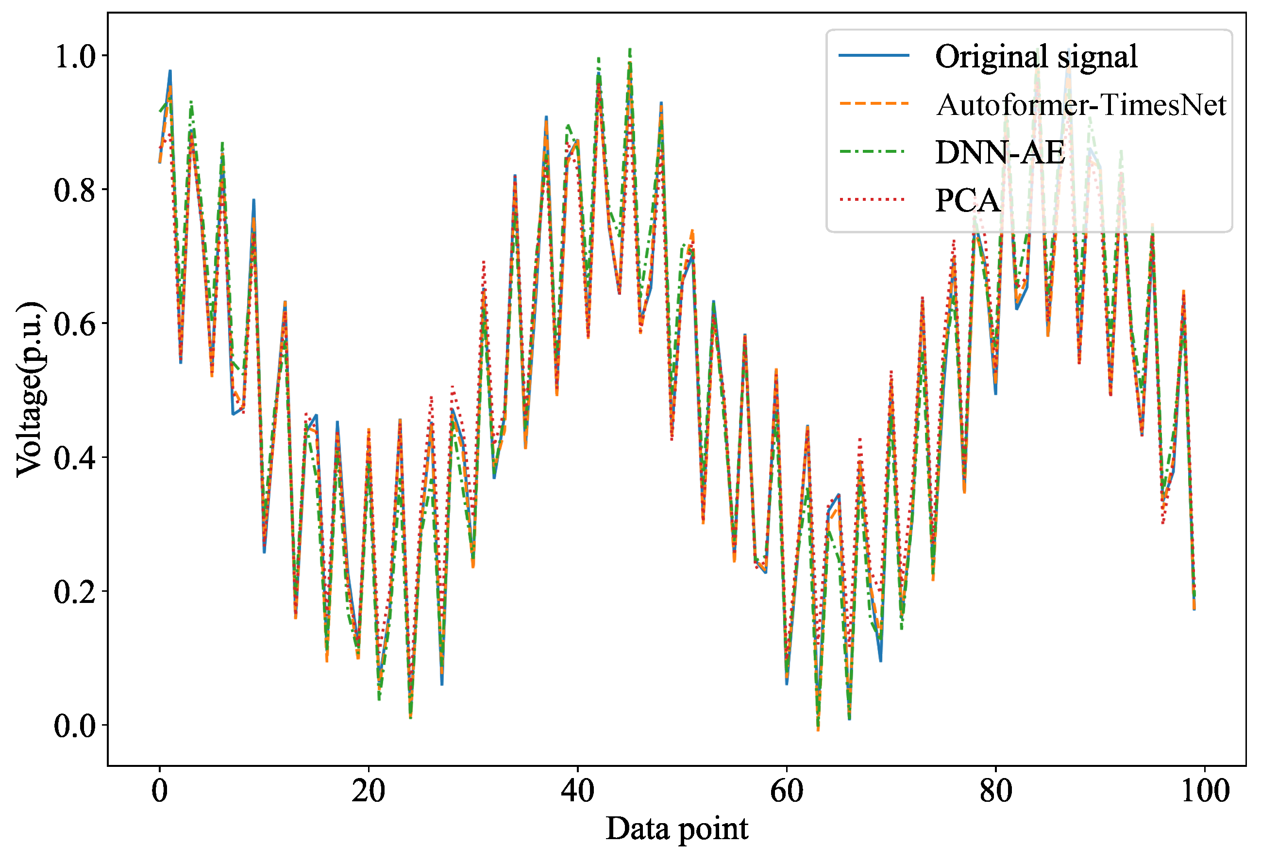
5.3. Signal Feature Extraction and Reconstruction Using Autoformer

In accordance with the Shannon sampling theorem, to fully reconstruct an original continuous signal from discrete samples, the sampling frequency must exceed twice the highest frequency of the original signal. Consequently, substations typically employ a higher sampling frequency to maximize the fidelity of the reconstructed signal. However, given the constraints on transmission rates, it is essential to transmit the data features collected by substations to the main station efficiently. In the simulation, a data sampling rate of 1000 Hz is set, and the dimensionality of the data after a reduction or decomposition is set to 7. Figure 6 and Figure 7 illustrate the restored voltage signals of non-oscillating and oscillating nodes using principal component analysis (PCA), density neural network autoencoder (DNN-AE), and Autoformer-TimesNet.

From Figure 6 and Figure 7 and

Table 1. Reconstruction of mean squared error (MSE) of different algorithms.

Method	MSE
Autoformer-TimesNet	$1.693\times {10}^{-4}$
DNN-AE	$1.839\times {10}^{-3}$
PCA	$1.120\times {10}^{-2}$

, it is evident that the reconstructed signal using the Autoformer-TimesNet algorithm most closely approximates the original signal, exhibiting the smallest reconstruction mean squared error (MSE). This superior performance is attributed to Autoformer-TimesNet’s unique temporal Auto-Correlation mechanism, which effectively captures long-term dependencies within sequences. With identical hidden layer dimensions, Autoformer-TimesNet demonstrates superior capability in extracting data features, resulting in a reconstructed signal that more accurately reflects the true signal. Conversely, the DNN-AE algorithm is unable to capture the relationships between long-term sequence data, leading to a higher reconstruction error compared to Autoformer-TimesNet. PCA, on the other hand, performs dimensionality reduction based on linear relationships in the data, disregarding minor components of variance, which results in the highest reconstruction error. Furthermore, in the reconstruction of oscillatory nodes, the Autoformer-TimesNet algorithm successfully recovers the voltage information of oscillatory nodes from the hidden layer data, avoiding misclassification, such as non-oscillatory nodes.

5.4. Oscillation Source Localization Based on Autoformer-TimesNet

Based on the hidden layer features extracted by Autoformer-TimesNet, further localization of wide-frequency oscillation disturbance sources is performed. To evaluate the effectiveness of the features extracted by Autoformer-TimesNet and the advantages of the CNN classification network, comparisons were made against a direct input of raw signals into the classification network and the use of DNN, RF, and SVM classification methods. The accuracy and training time for each algorithm on the test set are detailed in

Table 2. Comparison of wideband oscillation localization algorithms.

Features Dimension	Method	ACC	Time/s
7	Autoformer-TimesNet	0.9878	9.12
	DNN	0.9329	13.77
	RF	0.9123	2.01
	SVM	0.7386	1.03
100	Autoformer-TimesNet	0.9586	18.49

.

As shown in Table 2, ACC denotes the average accuracy of disturbance source localization for each method across 819 oscillation scenarios. These scenarios encompass 21 oscillation modes for each of the 39 nodes, spanning multiple frequency bands. The Autoformer-TimesNet classification network with feature extraction achieves the highest accuracy and positioning precision. Compared to directly inputting the raw signals without feature extraction, it not only yields higher accuracy but also requires less training time. This is because feature extraction preserves the most significant parts of each signal, preventing the neural network from learning irrelevant features, thus enhancing the neural network’s training efficiency. Additionally, the substantial reduction in feature dimensions effectively shortens training time.

To further verify the rationality and effectiveness of the algorithm’s feature extraction part, the sequences after feature extraction are fed into various machine learning models, such as deep neural networks (DNNs), random forest (RF), and support vector machines (SVMs). The performance of these models using the extracted features is compared with their performance using the original signals. Details on the accuracy and training time for each algorithm on the test set can be found in

Table 3. Comparison of raw data and feature-extracted data using different algorithms.

Method	Raw Data		Feature-Extracted Data
	ACC	Time/s	ACC	Time/s
DNN	0.9329	13.77	0.9435	11.27
RF	0.9123	2.01	0.9312	1.73
SVM	0.7396	1.03	0.8043	0.78

.

As shown in Table 3, we can clearly see that the performance of the three algorithms (DNN, RF, SVM) has significantly improved with the feature-extracted data compared to the raw data. In the case of feature-extracted data, both the accuracy and efficiency of these algorithms were enhanced to varying degrees. Specifically, the accuracy of the DNN increased from 0.9329 to 0.9435, and the training time decreased from 13.77 s to 11.27 s. The accuracy of the random forest (RF) increased from 0.9123 to 0.9312, and the training time decreased from 2.01 s to 1.73 s. The accuracy of the support vector machine (SVM) increased from 0.7396 to 0.8043, and the training time decreased from 1.03 s to 0.78 s. These results demonstrate that the feature extraction step not only improved the predictive accuracy of the models but also significantly reduced the training time, proving the effectiveness and superiority of the feature extraction method.

When comparing the Autoformer-TimesNet classification network with other algorithms, its accuracy remains the highest. This is due to Autoformer-TimesNet’s ability to share parameters through convolution kernels, which not only allows the integration of features from adjacent buses to enhance the classification accuracy but also reduces the number of neural network parameters. This reduction in parameters decreases the model’s complexity and effectively lowers the risk of overfitting. In contrast, the RF algorithm is sensitive to the selection of tree depth and the number of trees, leading to a higher likelihood of overfitting. The SVM algorithm is sensitive to kernel function selection and is not well suited for multi-classification problems, resulting in the poorest performance.

6. Conclusions

This paper extracts features from the original wide-frequency oscillation signals using the Autoformer-TimesNet neural network and converts them into two-dimensional data, thereby constructing a wide-frequency oscillation localization model. The main conclusions are as follows:

(a)

Utilizing the superior long-sequence processing capability of Autoformer, combined with the unsupervised learning method of the encoder–decoder, the high-dimensional original wide-frequency oscillation signals are decomposed into low-dimensional trend features and periodic features. This not only reduces the requirements for signal transmission rates but also lowers the difficulty and training time for wide-frequency oscillation localization.

(b)

Based on TimesNet, using the periodic features obtained from Autoformer decomposition as the input, Fourier decomposition is employed to determine the signal deformation basis. The deformed data can then be processed using models with local perception capabilities, such as CNNs. By sharing information between adjacent nodes, the localization accuracy is significantly improved.

(c)

Using CloudPSS to build an IEEE39 node simulation example, wide-frequency oscillation samples were generated by connecting wind turbines at different nodes. Further training of the Autoformer-TimesNet feature extraction network and wide-frequency oscillation localization network demonstrated that Autoformer-TimesNet can effectively extract features from the original signals, significantly reduce data dimensions, and improve the localization accuracy while reducing training time compared to other algorithms.

References

1. Du, E.; Zhang, N.; Hodge, B.M.; Wang, Q.; Kang, C.; Kroposki, B.; Xia, Q. The role of concentrating solar power toward high renewable energy penetrated power systems. IEEE Trans. Power Syst. 2018, 33, 6630–6641. [Google Scholar] [CrossRef]
2. Vicente, M.; Imperadore, A.; Correia da Fonseca, F.X.; Vieira, M.; Cândido, J. Enhancing Islanded Power Systems: Microgrid Modeling and Evaluating System Benefits of Ocean Renewable Energy Integration. Energies 2023, 16, 7517. [Google Scholar] [CrossRef]
3. Cheng, P.; Pan, T.; Li, R.; Liang, N. Research on optimal matching of renewable energy power generation system and ship power system. IET Renew. Power Gener. 2022, 16, 1649–1660. [Google Scholar] [CrossRef]
4. Olabi, A. Renewable energy and energy storage systems. Energy 2017, 136, 1–6. [Google Scholar] [CrossRef]
5. Shirkhani, M.; Tavoosi, J.; Danyali, S.; Sarvenoee, A.K.; Abdali, A.; Mohammadzadeh, A.; Zhang, C. A review on microgrid decentralized energy/voltage control structures and methods. Energy Rep. 2023, 10, 368–380. [Google Scholar] [CrossRef]
6. Jia, K.; Liu, C.; Li, S.; Jiang, D. Modeling and optimization of a hybrid renewable energy system integrated with gas turbine and energy storage. Energy Convers. Manag. 2023, 279, 116763. [Google Scholar] [CrossRef]
7. Liang, X. Emerging power quality challenges due to integration of renewable energy sources. IEEE Trans. Ind. Appl. 2016, 53, 855–866. [Google Scholar] [CrossRef]
8. Ju, Y.; Liu, W.; Zhang, Z.; Zhang, R. Distributed three-phase power flow for AC/DC hybrid networked microgrids considering converter limiting constraints. IEEE Trans. Smart Grid 2022, 13, 1691–1708. [Google Scholar] [CrossRef]
9. Kroposki, B.; Johnson, B.; Zhang, Y.; Gevorgian, V.; Denholm, P.; Hodge, B.M.; Hannegan, B. Achieving a 100% renewable grid: Operating electric power systems with extremely high levels of variable renewable energy. IEEE Power Energy Mag. 2017, 15, 61–73. [Google Scholar] [CrossRef]
10. Adefarati, T.; Bansal, R.C. Integration of renewable distributed generators into the distribution system: A review. IET Renew. Power Gener. 2016, 10, 873–884. [Google Scholar] [CrossRef]
11. Zhang, C.; Su, T.; Yuan, Z.; Zi, P.; Wu, L.; Wang, X. Research on Wideband Oscillation and Suppression Measure in PMSG-Based Wind Farm with SVG. In Proceedings of the 2023 IEEE International Conference on Power System Technology (PowerCon), Jinan, China, 21–22 September 2023; pp. 1–7. [Google Scholar]
12. Zong, H.; Lyu, J.; Wang, X.; Zhang, C.; Zhang, R.; Cai, X. Grey box aggregation modeling of wind farm for wideband oscillations analysis. Appl. Energy 2021, 283, 116035. [Google Scholar] [CrossRef]
13. Xu, Q.; Ma, Z.; Li, P.; Jiang, X.; Wang, C. A Refined Taylor-Fourier Transform with Applications to Wideband Oscillation Monitoring. Electronics 2022, 11, 3734. [Google Scholar] [CrossRef]
14. Lu, X.; Xiang, W.; Lin, W.; Wen, J. Analysis of wideband oscillation of hybrid MMC interfacing weak AC power system. IEEE J. Emerg. Sel. Top. Power Electron. 2020, 9, 7408–7421. [Google Scholar] [CrossRef]
15. Li, Y. An adaptive method for oscillations monitoring in power systems with high penetration of renewable energy. J. Physics Conf. Ser. IOP Publ. 2023, 2589, 012039. [Google Scholar] [CrossRef]
16. Li, C.; Yang, Y.; Dragicevic, T.; Blaabjerg, F. A new perspective for relating virtual inertia with wideband oscillation of voltage in low-inertia DC microgrid. IEEE Trans. Ind. Electron. 2021, 69, 7029–7039. [Google Scholar] [CrossRef]
17. Feng, S.; Cui, H.; Lei, J.; Yang, H.; Tang, Y. Data-Driven Time-Frequency-Domain Equivalent Modeling of Wind Farms for Wideband Oscillations Analysis. IEEE Trans. Power Deliv. 2023, 38, 4465–4475. [Google Scholar] [CrossRef]
18. Rao, Y.; Lyu, J.; Cai, X. Wideband impedance online identification of wind farms based on combined data-driven and knowledge-driven. In Proceedings of the 2022 IEEE International Power Electronics and Application Conference and Exposition (PEAC), Guangzhou, China, 4–7 November 2022; pp. 533–538. [Google Scholar]
19. Zhou, X.; Ma, H.; Wu, C.; Cheng, D.; Zhou, C.; Zheng, Z.; Wang, Y.; Jiang, Q. Wide-band Oscillation Disturbance Source Location Based on Compressed Sensing and CNN-LSTM. In Proceedings of the IEEE 7th Conference on Energy Internet and Energy System Integration (EI2), Hangzhou, China, 15–18 December 2023; pp. 4929–4934. [Google Scholar]
20. Wang, B.; Sun, K. Location methods of oscillation sources in power systems: A survey. J. Mod. Power Syst. Clean Energy 2017, 5, 151–159. [Google Scholar] [CrossRef]
21. Guo, S.; Zhang, S.; Li, L.; Song, J.; Zhao, Y. An Oscillation Energy Calculation Method Suitable for the Disturbance Source Location of Generator Control Systems. J. Phys. Conf. Ser. Iop Publ. 2020, 1518, 012081. [Google Scholar] [CrossRef]
22. Luan, M.; Gan, D.; Wang, Z.; Xin, H. Application of unknown input observers to locate forced oscillation source. Int. Trans. Electr. Energy Syst. 2019, 29, e12050. [Google Scholar] [CrossRef]
23. Feng, S.; Zheng, B.; Jiang, P.; Lei, J. A two-level forced oscillations source location method based on phasor and energy analysis. IEEE Access 2018, 6, 44318–44327. [Google Scholar] [CrossRef]
24. Li, L.; Wang, B.; Liu, S.; Li, J.; Teng, S.; Liu, D.; Peng, X.; Feng, S. Forced oscillation location based on temporal graph convolutional network. Energy Rep. 2023, 9, 646–654. [Google Scholar] [CrossRef]
25. Hu, W.; Lin, T.; Gao, Y.; Zhang, F.; Li, J.; Li, J.; Huang, Y.; Xu, X. Disturbance source location of forced power oscillation in regional power grid. In Proceedings of the 2011 IEEE Power Engineering and Automation Conference, Wuhan, China, 8–9 September 2011; Volume 2, pp. 363–366. [Google Scholar]
26. Wang, J. A novel oscillation identification method for grid-connected renewable energy based on big data technology. Energy Rep. 2022, 8, 663–671. [Google Scholar] [CrossRef]
27. Wang, S.; Lu, T.; Hao, R.; Wang, F.; Ding, T.; Li, J.; He, X.; Guo, Y.; Han, X. An Identification Method for Anomaly Types of Active Distribution Network Based on Data Mining. IEEE Trans. Power Syst. 2023, 39, 5548–5560. [Google Scholar] [CrossRef]
28. Liu, S.; Sun, K.; Zeng, C.; You, S.; Li, H.; Yu, W.; Deng, X.; Lin, Z.; Liu, Y. Practical Event Location Estimation Algorithm for Power Transmission System Based on Triangulation and Oscillation Intensity. IEEE Trans. Power Deliv. 2022, 37, 5190–5202. [Google Scholar] [CrossRef]
29. Yu, Y.; Min, Y.; Chen, L.; Zhang, Y. Disturbance source location of forced power oscillation using energy functions. Autom. Electr. Power Syst. 2010, 34, 1–6. [Google Scholar]
30. Li, W.; Guo, J.; Li, Y.; Zhou, X.; Chen, L.; Bu, G. Power system oscillation analysis and oscillation source location based on WAMS part 1: Method of cutset energy. Proc. CSEE 2013, 33, 41–46. [Google Scholar]
31. Estevez, P.G.; Marchi, P.; Galarza, C.; Elizondo, M. Complex dissipating energy flow method for forced oscillation source location. IEEE Trans. Power Syst. 2022, 37, 4141–4144. [Google Scholar] [CrossRef]
32. Ul Banna, H.; Solanki, S.K.; Solanki, J. Data-driven disturbance source identification for power system oscillations using credibility search ensemble learning. IET Smart Grid 2019, 2, 293–300. [Google Scholar] [CrossRef]
33. Gu, J.; Xie, D.; Gu, C.; Miao, J.; Zhang, Y. Location of low-frequency oscillation sources using improved DS evidence theory. Int. J. Electr. Power Energy Syst. 2021, 125, 106444. [Google Scholar] [CrossRef]
34. Matar, M.; Estevez, P.G.; Marchi, P.; Messina, F.; Elmoudi, R.; Wshah, S. Transformer-based deep learning model for forced oscillation localization. Int. J. Electr. Power Energy Syst. 2023, 146, 108805. [Google Scholar] [CrossRef]
35. Yang, L.; Wang, Y.; Gao, S.; Zheng, Z.; Jiang, Q.; Zhou, C. An Intelligent Location Method for Power System Oscillation Sources Based on a Digital Twin. Electronics 2023, 12, 3603. [Google Scholar] [CrossRef]
Figure 1. Structure diagram of Autoformer.
Electronics 13 03250 g001
Figure 2. Wideband oscillation periodic feature sequence decomposition and sequence folding.
Electronics 13 03250 g002
Figure 3. Extract features based on 2D convolution kernel.
Electronics 13 03250 g003
Figure 4. IEEE 39-bus system.
Electronics 13 03250 g004
Figure 5. Variation in reconstruction error with the number of hidden layers.
Electronics 13 03250 g005
Figure 6. Comparison of reconstructed signals at non-oscillatory nodes.
Electronics 13 03250 g006
Figure 7. Comparison of reconstructed signals at oscillatory nodes.
Electronics 13 03250 g007