An Effective and Robust Parameter Estimation Method in a Self-Developed, Ultra-Low Frequency Impedance Spectroscopy Technique for Large Impedances

Abstract

Bioimpedance spectrum (BIS) measurements are highly appreciated in in vivo studies. This non-destructive method, supported by simple and efficient instrumentation, is widely used in clinical applications. The multi-frequency approach allows for the efficient extraction of the most information from the measured data. However, low-frequency implementations are still unexploited in the development of the technique. A self-developed BIS measurement technology is considered the pioneering approach for low (<5 kHz) and ultra-low (<100 Hz) frequency range studies. In this paper, the robustness of ultra-low frequency measurements in the prototypes is examined using specially constructed physical models and a dedicated neural network-based software. The physical models were designed to model the dispersion mainly in the ultra-low frequency range. The first set of models was used in the training of the software environment, while the second set allowed a complete verification of the technology. Further, the Hilbert transformation was employed to adjust the imaginary components of complex signals and for phase determination. The findings showed that the prototypes are capable of efficient and robust data acquisition, regardless of the applied frequency range, minimizing the impact of measurement errors. Consequently, in in vivo applications, these prototypes minimize the variance of the measurement results, allowing the resulting BIS data to provide a maximum representation of biological phenomena.

1. Introduction

Bioimpedance (BI) measurement is a well-known and commonly used non-destructive material investigation technique [1,2]. Besides being non-destructive, the method’s attractiveness arises from its relatively simple and cost-effective instrumentation requirements, easy mass production, and efficient implementation procedures [2]. BI methods hold the promise of creating a portable, wearable spectrometer capable of performing numerous measurements virtually and invisibly at any time of day, even during physical activity [3]. Consequently, there is great interest in in vivo BI measurements, especially in human studies [4,5].

The method’s popularity in this field depends on its ability to determine the in vivo body composition of test subjects using prototypes and commercially available devices that are simple, user-friendly, and highly standardized at the same time [1,2,6,7,8]. The body composition parameters that can be determined by BI measurements are extracellular fluid, intracellular fluid, total body water, fat mass, fat-free mass, etc. [4]. Monitoring these features provides new perspectives for valuable population studies in the field of public health [4]. For example, monitoring the whole-body content of multi-ethnic groups [9], integration into e-Health programs [10], application in the training of athletes [11], and other clinical applications [12] can be considered.

The implementation of modern BI measurements beyond a single frequency (50 kHz) supports multiple-frequency and BI spectrum-based data collection [4]. In such cases, an AC (alternating current) excitation signal at a very low amplitude is usually applied to dedicated surface electrodes through the biological system under investigation, while the other surface electrodes are used to record the parameters (potential or voltage) of the resulting electric field [4]. In the case of multi-frequency implementations, measurement systems have been developed to simultaneously apply several excitation signals of different frequencies, while others measure the BI spectrum using a swept sine signal [2,4]. BI spectroscopy (BIS) has several advantages over other technologies since it maximizes the amount of useful information extracted from the data to characterize biological structures [4]. The excitation frequency range for BIS equipment is usually systematically shifted between 5 kHz and a few hundred kHz [4]. Typically, the frequency domain below 5 kHz is referred to as the low-frequency range [4].

In this paper, measurements of high impedances are conducted to investigate whether the underlying BIS measurement procedure and the self-developed prototype are capable of detecting model parameters as accurately as possible over the full frequency range. In order to accomplish these tasks, a new neural network-based data processing software is developed. The neural networks have already been used to estimate the parameters of the impedance spectrum in solving the inverse problem [13]. In addition, the Hilbert transformation has been used for parameter estimation involving neural networks [14]; however, it has not been used for spectroscopic inverse problem solutions. When the Hilbert transformation is applied, it ensures that the corresponding real and imaginary components of the impedance spectra are appropriately selected during the optimization process. Selecting the real and imaginary spectra in this manner and then applying the inverse procedure results in a more accurate determination of the R and C values compared to not using the Hilbert transformation. This software extracts the model parameters from the imported BIS data. Based on [15], specific physical models have been developed that include the impedance of the excitation electrodes, as well as the impedance of the material under investigation based on the Cole–Cole model [16] for the realization of this study. Two groups of physical models, called phantoms, have been constructed. The first group is used for neural network training, while the second group is used to verify the accuracy and robustness of the technology through the integration of ultra-precise components. Besides developing BIS technology, application development is also actively in progress, which will lead to the primary use of self-developed prototypes in biotechnological and clinical applications.

2. Related Works

In the following section, a brief review of the relevant literature is presented. State-of-the-art in vivo BI measurement systems incorporate, naturally, multi-frequency operation, and the latest tendency is the development of hardware miniaturization and wearable systems [3]. In the clinical routine, in vivo hemodialysis [17] and, of course, body composition [4,5] monitoring devices have already appeared, which also allow the examination of individual body segments [18]. Wearable BIS devices are increasingly appearing in new areas such as muscle [3], human skin Pelotherapy effects [19], body fat percentage and glucose levels [20], or even smartwatch-based [21] monitoring systems.

An outstanding application for this study is human muscle in vivo studies [22], where BIS systems operating at low (<5 kHz) frequencies are often applied and not only in wearable form [22]. In the low-frequency ranges, where the so-called α-dispersion can be detected, the ionic diffusion of the cell membrane and the counterion effects can be investigated [23]. Pislaru-Danescu et al. [23] recognized the potential of low-frequency measurements and new perspectives, proposing a prototype with gold electrodes for the investigation of different human body segments in their publication. Scaliusi et al. also presented a prototype operating mostly below 50 kHz to monitor edema in the human leg using wearable hardware [24].

However, at the same time, it cannot be ignored that although low-frequency measurements open up a new perspective for BIS applications, it is in many ways a more difficult engineering challenge to create a precise and accurate instrument in this frequency range [24,25]. In addition to explaining the operation of the prototypes, Scaliusi et al. [24,25] provided a passive electrical model of the complete measurement system (electrodes and test material). Similarly, the impedance of the electrodes and the measuring wires are represented by RC components, suggesting that they may cause a significant error in the measurement data at low frequencies [24,25]. These effects are collectively referred to as errors caused by residual impedances.

Consequently, the BI measurements are unique because they detect not only the signal of the unknown material sample but also the impedance of the measuring circuit and even of the components of the instrument [24,25]. A further almost impenetrable problem is that the effect of the measurement artifacts also depends on the unknown impedance [24,25]. In general, however, research on the technology today is still focused on improving the signal-to-noise ratio and minimizing measurement artifacts [1,2]. The pure basic research described in our proposal aims to reverse this trend by placing the technology on a new measurement and mathematical basis [1,2]. Despite the great potential of the technology, BI methods today still have several technological limitations [1,2]. El Khaled et al. [26] described an exponential increase in the number of publications on BI over the last decade. Nevertheless, it can be stated that the technology is stagnating and there is a very strong demand for real basic research on the technology [26,27].

The authors of the current publication have been continuously improving a self-developed BI measurement technique over the last 10 years [28,29]. This special, modified four-electrode technique is designed to generate data with a low measurement using the minimal data processing procedure. This novel measurement technique is a potential comparison technique that can be successfully applied independently from the application of a current or voltage generator. The essence of the method is to obtain the unknown impedance from the measured potentials by comparing it with the reference resistance. Thus, by taking the difference of the measured potentials, common mode rejection is achieved to minimize measurement errors and to suppress artifacts. The self-developed prototypes use this ground-breaking technique to measure at excitation frequencies between 1 mHz and 100 kHz, primarily to detect dispersion phenomena in the ultra-low (<100 Hz) frequency range of the substances. Nearly a decade of engineering research has resulted in a number of prototypes, which have been used to combine the experience gained with the construction of an ultra-precise digital lock-in amplifier with outstanding features.

The applications being developed by the authors are mainly oriented towards in vivo applications [28,30,31] of BIS measurements in addition to tomographic approaches [32]. For each of these applications, the measurement solutions are based on monitoring the α-dispersion (<100 Hz). In addition to the challenges of accurately realizing ultra-low frequency measurements, the impedance values to be measured usually vary over large ranges with high dynamic ranges (e.g., 100 kOhm–10 MOhm). All this concludes that effective and robust BIS measurements at ultra-low frequencies still remain a challenge for engineers involved in development today due to the residual impedances at low frequencies and the very high impedance values created by the polarization of biological structures [15,31]. In this paper, a technological approach is presented that is able to overcome these problems and provide the possibility of a reliable BIS measurement.

3. Materials and Methods

3.1. BIS Measurement Method

The BIS measurements utilize the modified four-electrode method presented in [15]. This specialized voltage comparison technique can be applied to both current and voltage generators. The core idea behind this implementation is to simultaneously suppress the high impedance (at low frequencies) of the excitation electrodes and the parasitic impedances of the measurement system during the measurement process. Consequently, this BI measurement technology is capable of eliminating the measurement artifacts discussed in Section 2, even at frequencies below 1 Hz, ensuring extremely accurate measurements. The technique achieves common-mode rejection of measurement artifacts by connecting the ground electrode directly to the measured material through a resistor, which raises the potential by a constant value. When calculating the impedance values, dividing the corresponding voltage and current values, along with eliminating the constant shift, results in highly efficient error suppression. Therefore, even at ultra-low frequencies (<10 Hz), the electrical properties of the measured material can be accurately recorded. The technology under investigation is a BI measurement system (Figure 1) developed by Vizvari et al. [15].

The self-developed digital lock-in algorithm, which was built into the instrument, was developed and improved by further development of the software in [33] (especially with respect to measurement noise) for the four-channel instrument. Lock-in amplifiers detect the measured signal only in the immediate area close to the user-defined reference frequency while suppressing other frequency components very effectively. Hence, lock-in amplifiers can determine the amplitude and phase of the measured signal almost exclusively at the frequency of the excitation signal, even in cases of extremely poor signal-to-noise ratios [33]. However, the use of lock-in amplifiers is routine in the realization of multi-frequency BI measurements [2]. Therefore, the system presented in this paper has outstanding capabilities for ultra-low frequency measurements. The system is designed with the following properties:

• two sampling frequencies are used: in the range 10 kHz–100 kHz, fs = 375 kSample/s, while in the frequency range 1 mHz–10 kHz, the signals are sampled at fs = 37.5 kSample/s. If fs = 375 kSample/s is used, the data management of the real-time calculations is achieved by ping-pong buffering,
• in each decade, the number of excitation frequencies can be selected between three and 100 (the frequency values are selected at equal distances from the logarithmic scale),
• different integration times are used for each frequency, hence the duration of the measurements is different for each frequency decade,
• an excitation signal of the sinusoidal waveform in the frequency range from 1 mHz to 100 kHz with a Total Harmonic Distortion plus Noise (THDN+N) suppression greater than 100 dB,
• the excitation is generated by a voltage generator with a maximum noise of 1.5 = µV_rms in the frequency range from 1 mHz to 100 kHz,
• the maximum excitation voltage is 10 V peak-to-peak, which can be reduced by up to 110 dB (i.e., up to about 32 µV peak-to-peak),
• the precision (variance) of the measured data is better than 1 ppm for amplitude and better than 0.01° for phase (demonstrated in [29]).

The measuring system’s compact dimensions (height: 55 mm, width: 100 mm, length: 170 mm) allow easy manual measurements. The robust construction and battery operation provide precise measurements. The maximum operating time of the measuring system is 6.5 h.

The BI measurement method implemented by the prototype (Figure 1) is the modified four-electrode technique developed by Vizvari et al. [29], which has been successfully applied in a variety of research. A schematic of the modified four-electrode measurement principle is shown in Figure 2.

The purpose of the measurement is to determine the Z_body impedance value at several frequency points. The method is based on connecting the ground point (0 V) of the measuring system directly to the measured sample, and then recording the measured data (potential values) to this ground point during the data acquisition process. The efficiency of the method can be increased by incorporating a shunt resistor (R_ref). During data processing, the unknown impedance (Z_body) is obtained by comparison with the shunt resistor using the following calculation:

$$Z_{body}={\displaystyle \frac{u_2-u_3}{u_4}}\cdot R_{ref}$$

(1)

The excitation of the test sample object is performed using a voltage generator, and the potential values $u_2, u_3$, and $u_4$ are measured. The accuracy and efficiency of the method come from the digital subtraction in Equation (1) of these potential data, which allows the method to significantly reduce the various errors in the measured data (using symmetrically balanced hardware).

In a previous study [29], the effectiveness of the measurement principle and its precision is demonstrated. In addition, further information can be found in [15].

3.2. BIS Phantoms

Previously [15], in order to demonstrate the advantageous properties of the technology, a physical model (BIS phantom) was created and applied. The phantoms were designed following the work of Fu et al. [27]. In this case, by evaluating the high-purity data collected during the measurement, the aim is to determine the model parameters of the different phantoms, i.e., the values of the electronic components (resistors and capacitors). By comparing the parameters extracted from the measurements with the values of the components used to make the phantoms, the accuracy and precision of the measurement procedure can be estimated.

The main aim of the phantom’s design was to mimic the ultra-low frequency dispersion as accurately as possible, together with the measurement-related artifacts that may result from, for example, the high impedance of the electrodes. The phantom (Figure 3) is a passive electrical circuit that produces a typical ultra-low frequency impedance spectrum. The phantom shown in Figure 3 is built from commercially available resistors and capacitors.

The objective of this study is to measure the (Z_body), which includes resistive (R) and capacitive (C) elements, through single-pole, two-pole, and three-pole approximations. Additionally, the measurement results are influenced by the excitation contacts (Z_in and Z_out), whose effects are variable and unknown. In order to characterize the model parameters, it is necessary to estimate the $R_0, R_{\infty }$, and $C$ values from the measurement results.

In order to develop a robust algorithm, the system was simulated using phantom models that employ single-pole and two-pole circuits. Initially, the behavior of the cell culture with a single-pole model is approximated. The phantom includes R-C elements in order to simulate the excitation path. The schematic diagram of the phantom circuit is shown below.

In Figure 2 and Figure 3, the voltages and their phases at points $u_2$, $u_3$, and $u_4$ can be measured with precision impedance measurement instruments. In total, 38 phantoms have been created for the current study. The key aspect in the design of these phantoms was ensuring that the generated pole and zero frequencies spanned nearly the entire frequency range (

Table 1. Specification of Measurements Circuits.

Phantom Number	Rin [kΩ]	Cin [uF]	R∞ [kΩ]	R0-R∞ [kΩ]	R0 [kΩ]	C [uF]	Rout [kΩ]	Cout [uF]
01	100	1	1	1	2	0.47	100	1
02	10	10	1	3.7	4.7	2.2	10	10
03	30	1	1	10	11	9.1	30	1
04	50	0.1	1	18	19	56	50	0.1
05	75	1	1	27	28	370	75	1
06	100	1	1	1	2	370	10	10
07	200	0.1	1	2.7	3.7	0.2	75	10
08	5	30	1	4.1	5.1	1	50	1
09	10	0.2	1	6	7	500	30	5
10	30	20	1	9	10	250	20	2
11	50	0.5	1	13	14	3	10	3
12	75	10	1	20	21	6	5	3
13	100	1	1	30	31	150	200	2
14	200	5	1	45	46	90	10	5
15	5	2	1	67	68	12	30	1
16	10	3	1	99	100	20	20	10
17	30	3	1	81	82	0.1	50	0.5
18	50	2	1	55	56	47	75	20
19	75	5	1	25	26	4.7	100	0.2
20	100	1	1	11	12	100	20	30
21	200	10	1	5	6	75	30	0.1
31	100	100	102	210	312	0.0002	100	100
32	100	100	93	402.1	495.1	0.0022	100	100
33	100	100	75	604	679	0.033	100	100
34	100	100	51.1	806	857.1	0.47	100	100
35	100	100	30.1	999.9	1030	0.94	100	100
36	100	100	10	1000	1010	0.0002	100	100
37	100	100	30.1	805.9	836	0.0022	100	100
38	100	100	51.1	604	655.1	0.033	100	100
39	100	100	71.5	400.5	472.0	0.48	100	100

) of the measurement system, especially the ultra-low frequencies. This also allows the efficiency of the technology to be investigated over the entire frequency range, even for relatively high impedances.

The aim was to train a robust system that can accurately estimate the values of C and R₀ from these measured voltages, regardless of the values set for the resistances C_in, R_in, C_out, and R_out. The voltage measurements are taken at the following frequencies: fk = 10^{−1.8 + k0.2} and k = {0, 1, …, 33}, which logarithmically span from 0.016 Hz to 63,000 Hz across 34 values (see Table 2), and these are available for all the measurement samples. The angular frequency for each measurement is given as ω_k = 2πf_k.

The measurements were taken in the form of a complex number:

$$\begin{gathered} Z=a+bi \\ \left|Z\right|=\sqrt{a^2+b^2}, Re\left(Z\right)=a, Im\left(Z\right)=b \\ \theta ={\tan }^{-1}\left({\displaystyle \frac{b}{a}}\right) \end{gathered}$$

(2)

where |Z| is the magnitude and θ is the phase.

The impedance measurements were transformed as follows:

Table 2. Measurement points and their transformation (TR—used for training).

Abbreviation	Equation	Description	Unit	Usage
U1	U1 = a1 + b1i	See Figure 2, complex format	V
U2	U2 = a2 + b2i	See Figure 2, complex format	V
U3	U3 = a3 + b3i	See Figure 2, complex format	V
U4	U4 = a4 + b4i	See Figure 2, complex format	V
U1p4ph	$={\tan }^{-1}\left({\displaystyle \frac{Im\left(U_1·{U_4}^{*}\right)}{Re\left(U_1·{U_4}^{*}\right)}}\right)$	U1/U4 phase	Rad	TR
U2p4ph	$={\tan }^{-1}\left({\displaystyle \frac{Im\left(U_2·{U_4}^{*}\right)}{Re\left(U_2·{U_4}^{*}\right)}}\right)$	U2/U4 phase	Rad	TR
U3p4ph	$={\tan }^{-1}\left({\displaystyle \frac{Im\left(U_3·U_4^{*}\right)}{Re\left(U_3·{U_4}^{*}\right)}}\right)$	U3/U4 phase	Rad	TR
U32p4ph	$={\tan }^{-1}\left({\displaystyle \frac{Im\left(\left(U_2-U_3\right)·{U_4}^{*}\right)}{Re\left(\left(U_2-U_3\right)·{U_4}^{*}\right)}}\right)$	(U2 − U3)/U4 phase	Rad	TR
Log10(U1p4mag)	$={\log }_{10}\left({\displaystyle \frac{\left|U_1·U_4^{*}\right|}{\sqrt{a_4^2+b_4^2}}}\right)$	Logarithm transform of U1/U4 magnitude		TR
Log10(U2p4mag)	$={\log }_{10}\left({\displaystyle \frac{\left|U_2·{U_4}^{*}\right|}{\sqrt{a_4^2+b_4^2}}}\right)$	Logarithm transform of U2/U4 magnitude		TR
Log10(U3p4mag)	$={\log }_{10}\left({\displaystyle \frac{\left|U_3·{U_4}^{*}\right|}{\sqrt{a_4^2+b_4^2}}}\right)$	Logarithm transform of U3/U4 magnitude		TR
Log10(U32p4mag)	$={\log }_{10}\left({\displaystyle \frac{\left|\left(U_2-U_3\right)·{U_4}^{*}\right|}{\sqrt{a_4^2+b_4^2}}}\right)$	Logarithm transform of (U2 − U3)/U4 magnitude		TR

Table 2. Measurement points and their transformation (TR—used for training).

Abbreviation	Equation	Description	Unit	Usage
U1	U1 = a1 + b1i	See Figure 2, complex format	V
U2	U2 = a2 + b2i	See Figure 2, complex format	V
U3	U3 = a3 + b3i	See Figure 2, complex format	V
U4	U4 = a4 + b4i	See Figure 2, complex format	V
U1p4ph	$={\tan }^{-1}\left({\displaystyle \frac{Im\left(U_1·{U_4}^{*}\right)}{Re\left(U_1·{U_4}^{*}\right)}}\right)$	U1/U4 phase	Rad	TR
U2p4ph	$={\tan }^{-1}\left({\displaystyle \frac{Im\left(U_2·{U_4}^{*}\right)}{Re\left(U_2·{U_4}^{*}\right)}}\right)$	U2/U4 phase	Rad	TR
U3p4ph	$={\tan }^{-1}\left({\displaystyle \frac{Im\left(U_3·U_4^{*}\right)}{Re\left(U_3·{U_4}^{*}\right)}}\right)$	U3/U4 phase	Rad	TR
U32p4ph	$={\tan }^{-1}\left({\displaystyle \frac{Im\left(\left(U_2-U_3\right)·{U_4}^{*}\right)}{Re\left(\left(U_2-U_3\right)·{U_4}^{*}\right)}}\right)$	(U2 − U3)/U4 phase	Rad	TR
Log10(U1p4mag)	$={\log }_{10}\left({\displaystyle \frac{\left|U_1·U_4^{*}\right|}{\sqrt{a_4^2+b_4^2}}}\right)$	Logarithm transform of U1/U4 magnitude		TR
Log10(U2p4mag)	$={\log }_{10}\left({\displaystyle \frac{\left|U_2·{U_4}^{*}\right|}{\sqrt{a_4^2+b_4^2}}}\right)$	Logarithm transform of U2/U4 magnitude		TR
Log10(U3p4mag)	$={\log }_{10}\left({\displaystyle \frac{\left|U_3·{U_4}^{*}\right|}{\sqrt{a_4^2+b_4^2}}}\right)$	Logarithm transform of U3/U4 magnitude		TR
Log10(U32p4mag)	$={\log }_{10}\left({\displaystyle \frac{\left|\left(U_2-U_3\right)·{U_4}^{*}\right|}{\sqrt{a_4^2+b_4^2}}}\right)$	Logarithm transform of (U2 − U3)/U4 magnitude		TR

3.3. Simulation Model

A mathematical model in MATLAB R2023b was developed in order to express the complex impedance using complex numbers, where the real part represents the ohmic resistance and the imaginary part represents the reactance.

The mathematical model of the circuit shown in Figure 3 was implemented in the MATLAB environment. This model served two primary purposes:

• first, to verify the accuracy of the measurements and the selected R and C values,
• second, to generate a large training database necessary for training the estimation system.

These aspects are detailed in the following two subsections.

The outputs of the model include the calculated impedance values and the corresponding phase angles at different points in the circuit, providing a comprehensive dataset for both validation and training purposes.

The model relies on operations with complex numbers, a functionality that is well-supported in MATLAB. The inputs to the model are the following:

• input and output impedances: $R_{in} ,R_{out}, C_{in}, C_{out}$
• body model impedance: $R_{\mathrm{\infty }}, R_0, C$
• shunt resistance: $R_s=\mathrm{96,000} \mathsf{\Omega }$
• supply voltage: $U_1=12 \mathrm{V}$
• frequency series: $f=\left[\mathrm{63,000,\; 39,750}, \dots , 0.016\right] \mathrm{H}\mathrm{z}$

The equations for the impedances are described in Equation (3), Equation (4) is the current, and Equation (5) represents the voltages and their ratios.

$$\begin{gathered} Z_{in}\left(f\right)={\displaystyle \frac{1}{\frac{1}{R_{in}}+i2\pi f{C}_{in}}} \\ {Z}_{out}\left(f\right)={\displaystyle \frac{1}{\frac{1}{R_{out}}+i2\pi f{C}_{out}}} \\ {Z}_{body}\left(f\right)=R_{\infty }+{\displaystyle \frac{1}{\frac{1}{R_0-R_{\infty }}+i2\pi fC}} \end{gathered}$$

(3)

$$I={\displaystyle \frac{U_1}{Z_{in}+Z_b+Z_{out}}}$$

(4)

$$\begin{gathered} U_4=R_{s}I \\ {U}_3=\left(Z_{out}+R_s\right)I \\ {U}_2=\left(Z_b+Z_{out}+R_s\right)I \\ {U}_{32}=Z_{b}I \\ {U}_{1p4}={\displaystyle \frac{U_1}{U_4}} \\ {U}_{2p4}={\displaystyle \frac{U_2}{U_4}} \\ {U}_{3p4}={\displaystyle \frac{U_3}{U_4}} \\ {U}_{32p4}={\displaystyle \frac{U_{32}}{U_4}} \end{gathered}$$

(5)

3.4. Training Database

Using this model, a database is generated that is compatible with the measurements. This means that the same outputs were calculated (U_1p4, U_2p4, U_3p4, and U_32p4 in polar format, i.e., magnitude + phase form) at the same frequencies (Table 2), using the same supply voltage and shunt resistance (U1, Rs). However, the variable electronic components (R₀, C, R_in, R_out, C_in, and C_out) differ from those in the measurements and cover a slightly broader range. It was ensured that the training and validation datasets contained different R₀ and C values. This separation is crucial to ensure that the neural network (NN) model’s training and validation sets are independent of each other, preventing overfitting.

Table 3. Training database elements.

Element	Set	Size	Value set	Unit	m-Equation
Rin, Rout	TR	9	5, 10, 20, 30, 50, 100, 200, 300, 500	kΩ
	VA	7	7, 15, 25, 40, 75, 150, 250	kΩ
Cin, Cout	TR	7	0.1, 0.3, 1, 3, 10, 30, 100	µF
	VA	4	0.2, 2, 20, 200	µF
R0	TR	36	1.2, 1.5, 1.8, 2.2, 2.7, 3.3, 4.1, 5.0, 6.0, 7.4, 9.0, 11.0, 13.5, 16.4, 20.1, 24.5, 30.0, 36.6, 44.7, 54.6, 66.7, 81.5, 99.5, 121.5, 148.4, 181.3, 221.4, 270.4, 330.3, 403.4, 492.7, 601.8, 735.1, 897.8 1096.6, 1339.4	kΩ	Roundn (exp(0.2:0.2:7.2),−1) × 103
	VA	22	1.2, 1.6, 2.3, 3.2, 4.4, 6.2, 8.6, 12.0, 16.7 23.3, 32.6, 45.5, 63.4, 88.5 123.6, 172.4, 240.6, 335.9, 468.7, 654.1, 912.9 1274.1	kΩ	Roundn (exp(0.15:1/3:7.25),−1) × 103
C	TR	31	0.0001, 0.0002, 0.0003, 0.0006, 0.0009 0.0015, 0.0025, 0.0041, 0.0067, 0.0111, 0.0183, 0.0302, 0.0498, 0.0821 0.1353, 0.2231, 0.3679, 0.6065 1, 1.6487, 2.7183, 4.4817, 7.3891 12.182, 20.085, 33.115, 54.598, 90.017 148.41, 244.69, 403.43	µF	Roundn (exp(−9:0.5:6),−4) × 1 × 10−6
	VA	26	0.0002, 0.0003, 0.0005, 0.0009, 0.0017, 0.0030, 0.0055, 0.0101, 0.0183, 0.0334, 0.0608 0.1108, 0.2019, 0.3679, 0.6703 1.2214, 2.2255, 4.0552, 7.3891 13.464, 24.532, 44.701, 81.451 148.41, 270.43, 492.75	µF	Roundn (exp(−8.8:0.6:6.2),−4) × 1 × 10−6
Rs	-	1	96	kΩ
$R_{\infty }$	TR	11	1, 1.6, 2.7, 4.5, 7.4 12.2, 20.1, 33.1, 54.6, 90, 148.4	kΩ	Roundn (exp(0:0.5:5),−1) × 103
	VA	8	1.2, 2.5, 5 10, 20.1, 40.4, 81.5, 164	kΩ	Roundn (exp(0.2:0.7:5.2),−1) × 103

summarizes the statistics of the generated database. The datasets were generated using a combinatorial approach, where every value of R_in and C_in with every value of R₀ and C were combined. Consequently, the sizes of the training (TR) and validation (VA) datasets are as follows:

$$\begin{gathered} n\left(TR\right)=n\left(Ri{n}_{TR}\right)·n\left(Ci{n}_{TR}\right)·n\left(R{0}_{TR}\right)·n\left(C_{TR}\right)=9·7·36·31=70308 \\ n\left(VA\right)=n\left(Ri{n}_{VA}\right)·n\left(Ci{n}_{VA}\right)·n\left(R{0}_{VA}\right)·n\left(C_{VA}\right)=7·4·22·26=16016 \end{gathered}$$

(6)

The $R_{\infty }$ was circularly repeated for each combination, but with constrains of $R_0>R_{\infty }$. The R_out and C_out values were not the same as R_in and C_in since they were chosen randomly from the same set of values. However, this random selection pattern remained consistent across all variations of R₀ and C.

3.5. Neural Network

A small convolutional neural network (CNN) with inputs consisting of various voltage ratios and outputs providing the estimated values of R₀, $R_{\infty }$, and C was designed. In order to make the neural network’s estimation system more linear, the network estimates the logarithm base log10 of the output values (log10(R₀), log10(R_∞), and log10(C)).

Two metrics were used in order to measure the performance:

• RMS: The root mean square error of the estimates [34].
• Pearson: The Pearson correlation coefficient of the estimates [35].

These metrics were calculated for either the training set (TR), the validation set (VA), or the test set (TE). The training and validation sets were generated through simulation, while the test set was derived from actual measurements.

A simple 10-layer CNN was designed for the regression task of estimating log10(R₀), log10(R_∞), and log10(C) (see Figure 4). The input layer accepts two sets of 34 polar numbers, derived from voltage measurements. Following the input layer, there are three convolutional layers with filter sizes of [15 1], [11 1], and [7 1] and corresponding filter counts of 24, 31, and 35, each followed by a Leaky ReLu activation function [36]. These layers are succeeded by two fully connected layers, the first with 126 units and the second with three units, representing the estimated R₀, R_∞, and C values. The training of this CNN is performed using the Adam optimizer [37], which ensures efficient and effective convergence during the learning process.

The Leaky ReLu is a parameterized ReLu layer, which works as follows [36]:

$$y=LeakyReLu\left(x,Alpha\right)=\left\{\begin{array}{cc}x& x>0\\ x·Alpha& x\le 0\end{array}\right.$$

(7)

The parameters of the CNN are organized in a structure named param, which is summarized in

Table 4. The CNN configuration.

NN Parameter	Description	Value Range	Initial	Optimum
Hilb	Hilbert Rule Control in complex input signals	0–0.3	0.05	0.1
convSize (1)	Filter size in convolution layer 1	10–25	20	15
convSize (2)	Filter size in convolution layer 2	7–18	14	11
convSize (3)	Filter size in convolution layer 3	3–10	5	7
numFilters (1)	Number of filters in convolution layer 1	10–40	25	24
numFilters (2)	Number of filters in convolution layer 2	10–40	25	31
numFilters (3)	Number of filters in convolution layer 3	10–40	25	35
leakyRelu (1)	Scale of leaky rectified linear unit layer 1	0–0.2	0.1	0.13687
leakyRelu (2)	Scale of leaky rectified linear unit layer 2	0–0.2	0.1	0.01749
leakyRelu (3)	Scale of leaky rectified linear unit layer 3	0–0.2	0.1	0.18037
fullySize (1)	Output size of fully connected layer 1	50–250	64	126
fullySize (2)	Output size of fully connected layer 2	3 (fix)	3	3
initLR	Initial Learn Rate	1 × 10−4:5 × 10−3	0.001	0.001
MiniBatchSize	number of samples used in each iteration of the training algorithm	50–400	128	103
LRdropfactor	Learn Rate Drop Factor—factor by which the learning rate is reduced during training at specified drop periods	0.3–0.9	0.6	0.35138
LRdropperiod	Learn Rate Drop Period	1 (fix)	1	1
MaxEpochs	maximum number of training epochs	7 (fix)	7	7

.

The NN parameters were optimized using a Particle Swarm Optimization (PSO) algorithm [38] in order to achieve the highest possible performance. The algorithm was developed and used in earlier research [39]. The resulting optimized parameters are listed in the last row of Table 3. Later, these parameters were used in training the final NN.

3.6. Hilbert Transformation Filter

The Hilbert transformation allows the generation of an analytic signal, which is valuable in telecommunications for bandpass signal processing, particularly referring to the continuous-time analytic signal [40,41,42]. An analytic signal is a complex-valued function with non-negative spectral components [41]. The real and imaginary parts of an analytic signal are real-valued functions related by the Hilbert transformation filter.

This technique is used to acquire the minimum-phase response from a spectral analysis, making it convenient for analyzing the signal phase [42]. The Hilbert transformation can estimate the phase and magnitude of an input signal [43,44,45,46,47,48]. A common method of phase reconstruction, based on the Hilbert transformation, can only reconstruct the interpretable phase from a limited class of signals, such as narrow-band signals [48].

In signal processing, the Hilbert transformation is a linear operator that obtains a function g(t) and creates a function H(g(t)) in the same domain [41,42,43,44,45]:

$$H\left(g\left(t\right)\right)=g\left(t\right)\ast {\displaystyle \frac{1}{\pi t}}={\displaystyle \frac{1}{\pi }}{\int }_{-\propto }^{\propto }{\displaystyle \frac{g\left(\tau \right)}{t-\tau }}d\tau$$

(8)

In Equation (8), H denotes the Hilbert transformation and * denotes the convolution operation.

In the frequency domain, the Hilbert transformation can be written as follows [41,42,43,44,45,46,47,48]:

$$F\left(H\left(g\left(t\right)\right)\right)=G\left(\omega \right)F\left({\displaystyle \frac{1}{\pi t}}\right)=G(\omega )H(\omega )$$

(9)

where “F” denotes the Fourier transform, and H(ω) can be calculated with the following expression:

$$F\left({\displaystyle \frac{1}{\pi t}}\right)=H\left(\omega \right)=-j sgn\left(\omega \right)=\left\{\begin{array}{c}-j, \omega >0\\ 0, \omega =0\\ j, \omega <0\end{array}\right.$$

(10)

The Hilbert transformation in the time domain results in a ${\displaystyle \frac{\pi }{2}}$ phase-shift operator between the input and output signal; therefore, it could be applied as a phase-shifting procedure in a defined bandwidth of interest [46,47,48].

Further, a standard method for reconstructing the instantaneous phase from a signal is based on the Hilbert transformation [44,46,48]. This method calculates the phase from the analytic signal:

$$\xi \left(t\right)=g\left(t\right)+j\left(H\right(g\left(t\right))$$

(11)

where g(t) is the observed signal, H(g(t)) is its Hilbert transformation, and ξ(t) is an analytic signal. Hence, for realizable systems, the Hilbert transform links the real and imaginary parts of the signal, with the imaginary part being the Hilbert transformation of the signal’s real part [44,45,46,47,48]. This is an important relationship that allows the analysis of the given signal g(t) through the Hilbert transformation. In addition, the Hilbert transformation is also employed to connect the gain and phase characteristics of linear communication channels and minimum-phase filters [45,47].

Thus, the Hilbert transformation reconstructs the instantaneous phase with the argument of the analytic signal (11) as follows:

$${\varphi }^H=\arg \left[\xi \left(t\right)\right]={tan}^{-1}{\displaystyle \frac{H\left(g\left(t\right)\right)}{g\left(t\right)}}$$

(12)

where ${\varphi }^H$ is the obtained phase using the Hilbert transformation [48].

Further, the instantaneous envelope or magnitude of the analytic signal is given as:

$${\left|\xi \right(t\left)\right|}^H=\sqrt{{\left(g\left(t\right)\right)}^2+{\left(H\right(g\left(t\right)\left)\right)}^2}$$

(13)

where ${\left|\xi \right(t\left)\right|}^H$ represents the obtained magnitude using the Hilbert transformation.

As can be seen in both, the envelope and phase are available as functions of time and if g(t) is known, then H(g(t)) can be calculated [44,45,46,47,48,49,50]. In certain applications, the instantaneous amplitude and phase often are utilized to measure and detect the local features of the signal, which can result in a correction of the signal itself using its real and imaginary parts [46].

The Hilbert transformation [40] was utilized in order to correct the imaginary parts of complex signals. Essentially, from the real part, the Hilbert transformation creates a quasi-imaginary signal, which is then used to slightly modify (by β = 10%) the original imaginary part. By including this modified complex voltage ratio signal into the neural network, better results can be achieved. If the Hilbert transformation is not used, the real and imaginary parts of the impedance are treated independently by the optimization procedure, without consideration of the physical relationship between them since there is nothing to connect them. Therefore, when the Hilbert transformation is used, it helps to ensure that the corresponding real and imaginary parts of the impedance spectra are selected during the optimization process [44,45,46,47,48]. The real and imaginary spectra selected in this way, when subjected to the inverse procedure, result in a better pair of R and C values than if the Hilbert transformation had not been used. This is also confirmed by the results presented later in

Table 5. RMS Error statistics of the best CNN instances, calculated between nominal values and estimated values in the logarithmic domain. R₀ and R_∞ are expressed as rms(log10(kΩ)) and C is expressed as rms(log10(µF)).

		TR			VA			TE
CNN Instance	Hilbert Filtering	R0	R∞	C	R0	R∞	C	R0	R∞	C
Initial CNN architecture (cnn_init_ch_U32p4)	No	0.014	0.047	0.070	0.021	0.039	0.072	0.032	0.024	0.175
Initial CNN architecture (cnn_init_ch_U32p4U32p4x)	Yes	0.012	0.045	0.068	0.018	0.033	0.075	0.033	0.020	0.146
Optimized CNN architecture (cnn_opt_ch_U32p4)	No	0.012	0.046	0.073	0.019	0.037	0.072	0.033	0.020	0.155
Optimized CNN architecture (cnn_opt_ch_U32p4U32p4x)	Yes	0.010	0.042	0.069	0.014	0.038	0.065	0.030	0.017	0.143

. It is particularly interesting that, even without optimization, the R and C values derived from the real and imaginary spectra linked by the Hilbert transformation are better than those obtained without using the Hilbert transformation. The U_32p4x is derived from the U_32p4 measured complex signal as follows (14):

$$\begin{gathered} U_{32p4}=a+bi \\ {U}_{32p4x}=a+\left(\left(1-\beta \right)b+\beta H\left(a\right)\right)i \end{gathered}$$

(14)

where the H is the Hilbert transformation, a and b represent the real and imaginary parts of the signal, respectively, and β is the modification factor.

Hilbert transformation helps with the accurate phase determination of the signal [44,45,46,47,48]. With the adjustment of the imaginary part of the complex signal using the Hilbert-transformed real part, phase errors can be achieved, leading to more accurate impedance measurements. Moreover, the inherent characteristics of the original signal are maintained by the Hilbert transformation, which slightly modifies the imaginary part (by 10% in this case). The use of the Hilbert transformation in the proposed methodology is not solely for noise reduction, but rather to leverage the relationship between the real and imaginary parts of the signal [49,50]. The Hilbert transformation applies a mathematical rule that inherently links the real and imaginary components, potentially enhancing the signal’s interpretability for the neural network. Even in synthetic data, this transformation can serve as a form of regularization, ensuring that the network learns a more generalized model that can handle variations in real-world data more effectively. This approach is based on the hypothesis that the Hilbert transformation helps the network to better understand the underlying phase relationships in the data, which are crucial for accurate impedance measurements [46,47,48]. By doing so, the essential properties of the original complex signal are retained while the influence of outliers and measurement errors is reduced.

4. Results

4.1. Verification of the Electronics Setup

Additionally, the model was used to perform calculations with the values corresponding to the measurements (Table 1) in order to assess the accuracy of the electronic boards compared to their nominal values. Figure 5 shows the statistical distribution of the RMS error calculated between the measurements and simulation. Figure 4 and Figure 5 represent two types of samples, relatively accurate and typical non-accurate samples.

The distribution shown in Figure 5 is calculated across the available measurements with the actual Phantom circuit.

These comparisons in Figure 6 and Figure 7 revealed that some electronic boards showed significant discrepancies between the measurement and simulation results, specifically phantom boards 4, 5, and 9. This suggests that the components on these electronic phantom boards do not match their nominal values for some reason, with a small likelihood that the measurement instrument itself is faulty. These boards were set aside for further inspection and they were excluded from further testing.

Additionally, new boards were fabricated (phantoms 31–38) and equipped with high-precision components, and such differences were no longer observed. This confirmed that the discrepancies were due to the wide tolerance ranges of the original electronic components.

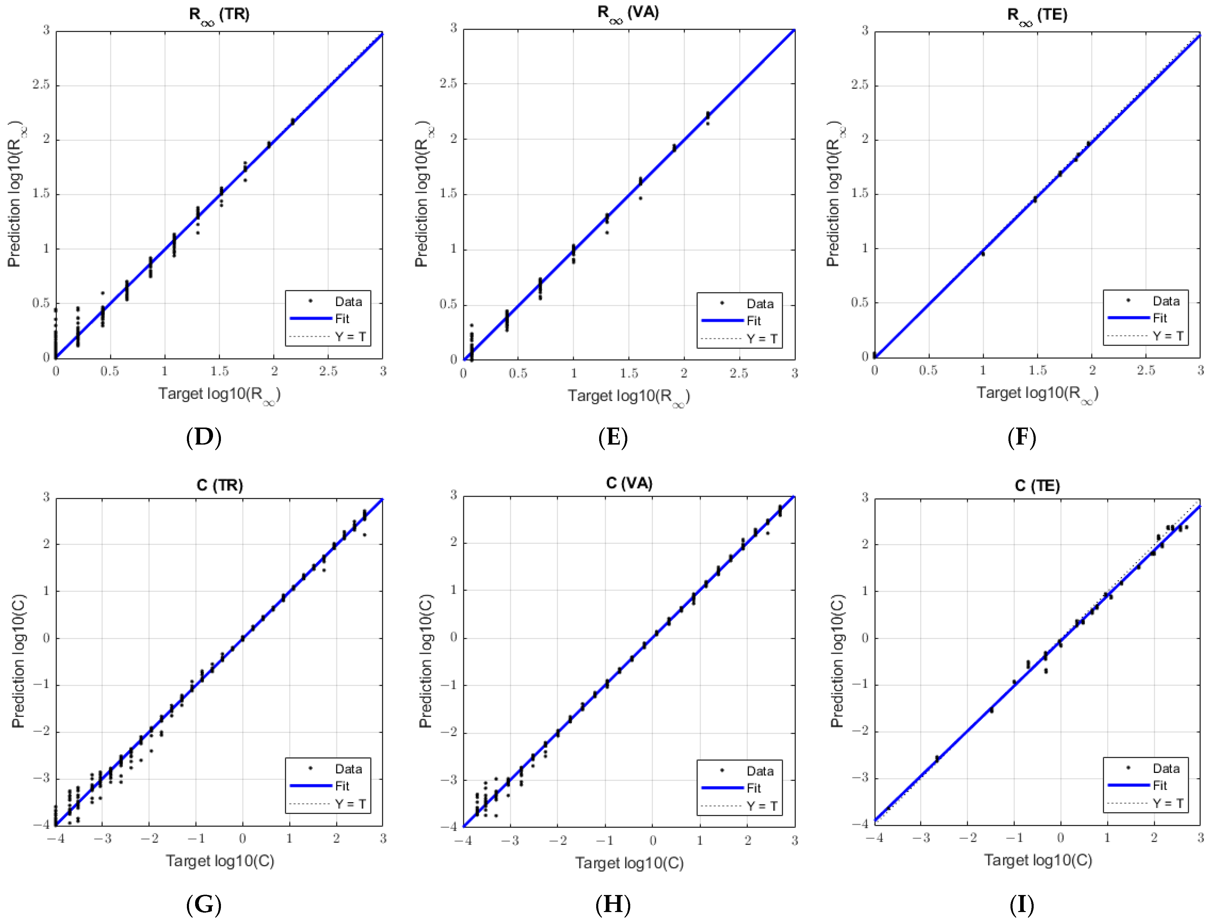
4.2. Estimation Results with Neural Networks

The neural networks were trained with several input signals (Table 2) in the first round of benchmarks. The network identified the key measurement input corresponding to the Z_body impedance voltage, specifically U₃₂, and its normalized form, U₃₂p4.

In the second round of the benchmark, the NN architecture and the hyperparameters were optimized, which are listed in Table 4.

The performance was improved when the network included these corrected measurements alongside the enhanced signals processed through the Hilbert filter. This approach ensures that the neural network receives more refined input data, leading to improved accuracy in estimating the resistance and capacitance values.

In Table 5, TR represents the results of the training set, VA represents the results of the validation set, and TE represents the results of the external test set (the real measurements). The measurement unit of resistance error (R₀ and R_∞) is log10(kΩ) and the measurement unit of capacitor error (C) is log10(µF). As shown in Table 5, the real and imaginary spectra selected through the proposed method yield a superior pair of R and C values when subjected to the inverse procedure compared to the results obtained without using the Hilbert transformation.

The best model has been selected as cnn_opt_ch_U32p4U32p4x. This NN model used, as inputs, the U₃₂/U₄ voltages in polar format (U_32p4) and their filtered version with Hilbert transformation (U_32p4x). The regression analysis is demonstrated in Figure 8. The typical error levels vary along the spectrum and the lower range of R_∞ and C are more difficult to estimate. In contrast, the higher range of R₀ has higher error levels. There are several larger errors in the external test statistics, especially at C, that were due to the Phantom circuits having uncertain values due to high tolerance electronic elements. The explanation of this error is discussed in Section 5.

Table 6. Small group of samples from the test set.

Record Name	R0 [kΩ]	Estimated R0 [kΩ]		R∞ [kΩ]	Estimated R∞ [kΩ]		C [uF]	Estimated C [uF]
	Nominal	Cnn_Opt_Ch_U32p4	Cnn_Opt_Ch_U32p4U32p4x	Nominal	Cnn_Opt_Ch_U32p4	Cnn_Opt_Ch_U32p4U32p4x	Nominal	Cnn_Opt_Ch_U32p4	Cnn_Opt_Ch_U32p4U32p4x
Fantom01_Extra00	2.0000	1.9508	1.9624	1.0000	0.9647	0.9674	0.4700	0.4872	0.4324
Fantom03_Extra1,10	11.0000	10.6626	10.8975	1.0000	0.9539	0.9789	9.1000	8.1631	8.8900
Fantom06_Extra10,12	2.0000	1.8970	1.9578	1.0000	0.9860	0.9716	370.0001	223.3616	248.9201
Fantom16_Extra14,10	100.0000	105.1268	107.6225	1.0000	0.9551	0.9880	20.0000	14.5450	17.4282
Fantom19_Extra14,11	26.0000	27.6678	27.6018	1.0000	0.9807	0.9882	4.7000	3.6715	3.9807
Fantom32 (2024-05-02_12-25-31)	495.1000	519.5878	577.8306	93.0000	89.2673	94.4957	0.0022	0.0058	0.0047

lists examples from the external set of measurements, showing the estimated or recovered values from the two optimized CNN models identified in Table 5. The variability between different neural network models can be observed in both resistor and capacitor estimations. Capacitor values are commonly estimated to be slightly lower than the nominal values, as seen in a logarithmic format in the graph in Figure 8I. This small bias is observed between the simulation and real measurements.

5. Discussion

The results presented so far are presented for measurements on BIS phantoms. The phantoms have been created to verify the accuracy of the modified four-electrode measurement procedure and the prototype was developed based on it, over the whole measurement frequency range, even when measuring high-value impedances. Measurement results on phantoms were evaluated using software specially designed for this purpose.

The neural network was trained on a large, simulated database. In the simulated data, there are no tolerance deviations, meaning that each sample is exact and noise-free. However, when running this estimation system on the external test database, the model relies solely on the trends and is likely to show more accurate resistance and capacitance values. This discrepancy arises since the nominal values are not always precise due to the components’ higher tolerance ranges. This result was validated using high-precision components on the last eight measurement boards, resulting in no significant deviations.

During the training phase, the minimum and maximum values of resistance and capacity were adjusted in order to match the first set of circuit boards (set 1–22). However, later, the need for a new set of circuit boards with more precise tolerance for the nominal values of resistance and capacity was identified in order to confirm the source of the deviation between simulations, based on nominal values and measurement. Unfortunately, only smaller capacity values were available for the target precision category. Consequently, the new boards (set 32–39) were created with different values compared to the original training dataset, with smaller capacity and higher resistance values in order to maintain the intended frequency range. This new set of circuit boards was added in the last phase of the research, and it was used as an external independent validation. The decision was not to retrain the CNN with the new data since the prediction was robust for the given ranges.

The error level of magnitude and phase curves remained consistently at 0.02 log10(V/V) magnitude error and 0.02 radians phase error (Figure 5). The neural network’s error margin aligns with these results: rms(log10(kΩ)) = 0.03 for R₀, rms(log10(kΩ)) = 0.017 for R₀, and rms(log10(µF)) = 0.143, as shown in Table 5. By adjusting the imaginary part of the complex signal using the Hilbert-transformed real part, phase errors can be reduced, resulting in more accurate impedance estimation, as was shown in the comparison between networks with and without Hilbert filtering, presented in Table 5.

The resistance estimation on external test measurements is two times higher compared to simulation validation (rms(log10(kΩ)) = 0.014 versus 0.030). Similarly, the capacitance estimation error on the external test measurements was significantly higher than simulation validation (rms(log10(µF)) = 0.065 versus 0.143) due to the circuits having large tolerance ranges.

The study findings suggest that in order to accurately measure performance, components with precisely known values (with 0.1% accuracy) must be chosen. This level of precision is crucial for ensuring that the system’s performance is measured correctly and that the resistance and capacitance values can be reliably estimated by the neural network in practical applications.

6. Conclusions

In this paper, self-developed BIS technology has been briefly presented and applied in practice. The investigation examines whether the impressive properties of the new technology are maintained over the entire operating frequency range (1 mHz–100 kHz). To this end, a BIS phantom has been developed and a significant quantity of these phantoms have been completed. Dedicated convolutional neural network-based software was developed in order to evaluate the measurement results. It estimates both the resistors and capacitors in a logarithmic format using the U₃₂/U₄ voltage ratio filtered with Hilbert transformation. The performance of this network reaches a high correlation (>0.99) with the reference values. Some of the phantoms were used to train this software and others were used in testing. The results are very impressive; the most impressive evidence of the cooperation between the measuring system and the measuring software is the fact that very small errors were observed in the extraction of model parameters for the test phantoms. As a result of the impedance spectrum measurement, either the real and imaginary parts of the impedance spectrum or their amplitude and phase characteristics are achieved. These curves are created using the measurement results at discrete frequency points. The fitting of these two curves occurs independently at these measurement points; either in the case of the real-imaginary pair or the amplitude-phase pair characteristics. Each fitting carries its own errors, as inverse procedures are sensitive to the initial data, thus an auxiliary condition that assists the inverse calculation process is beneficial. The auxiliary condition for the inverse procedure presented in this paper is provided by the Hilbert transformation. The Hilbert transformation, for realizable systems, connects the real and imaginary parts of the transfer function since the imaginary part is actually the Hilbert transformation of the real part. The CNN was trained with both real measurement results and numerical examples. The results have clearly presented that the application of the Hilbert transformation supports the inverse procedure. The accuracy of the circuit element values calculated using the inverse method was better even when the CNN was not optimized with the application of the Hilbert transformation, and after optimization, the accuracy became particularly good.

The results showed that the model parameters were successfully recovered over the full range of the measurement frequencies. Consequently, the presented BIS technology is recommended for human body composition and body segment composition studies at ultra-low frequencies, since even high impedances can be measured in this frequency range. Additionally, this technology could also be utilized for the detailed study of apoplastic fluid resistance in plants, providing valuable insights into plant physiology and water transport mechanisms.

References

1. Naranjo-Hernández, D.; Reina-Tosina, J.; Min, M. Fundamentals, recent advances, and future challenges in bioimpedance devices for healthcare applications. J. Sens. 2019, 2019, 9210258. [Google Scholar] [CrossRef]
2. Showkat, I.; Khanday, F.A.; Beigh, M.R. A review of bio-impedance devices. Med. Biol. Eng. Comput. 2023, 61, 927–950. [Google Scholar] [CrossRef] [PubMed]
3. Kusche, R.; Oltmann, A.; Rostalski, P. A Wearable Dual-Channel Bioimpedance Spectrometer for Real-Time Muscle Contraction Detection. IEEE Sens. J. 2024, 24, 11316–11327. [Google Scholar] [CrossRef]
4. Zachariah, V.K.; Priyamvada, P.S. Bioimpedance Analysis: Basic Concepts. J. Ren. Nutr. Metab. 2023, 8, 30–34. [Google Scholar] [CrossRef]
5. Aldobali, M.; Pal, K. Bioelectrical Impedance Analysis for Evaluation of Body Composition: A Review. In Proceedings of the 2021 International Congress of Advanced Technology and Engineering (ICOTEN), Taiz, Yemen, 4–5 July 2021; pp. 1–10. [Google Scholar]
6. Khalil, S.F.; Mohktar, M.S.; Ibrahim, F. The Theory and Fundamentals of Bioimpedance Analysis in Clinical Status Monitoring and Diagnosis of Diseases. Sensors 2014, 14, 10895–10928. [Google Scholar] [CrossRef]
7. Mialich, M.S.; Sicchieri, J.F.; Junior, A.J. Analysis of Body Composition: A Critical Review of the Use of Bioelectrical Impedance Analysis. Int. J. Clin. Nutr. 2014, 2, 1–10. [Google Scholar]
8. Matthie, J.R. Bioimpedance measurements of human body composition: Critical analysis and outlook. Expert Rev. Med. Devices 2008, 5, 239–261. [Google Scholar] [CrossRef]
9. Blue, M.N.M.; Tinsley, G.M.; Hirsch, K.R.; Ryan, E.D.; Ng, B.K.; Smith-Ryan, A.E. Validity of total body water measured by multi-frequency bioelectrical impedance devices in a multi-ethnic sample. Clin. Nutr. ESPEN 2023, 54, 187–193. [Google Scholar] [CrossRef]
10. El Dimassi, S.; Gautier, J.; Zalc, V.; Boudaoud, S.; Istrate, D. Mathematical Issues in Body Water Volume Estimation Using Bio Impedance Analysis in e-Health; Colloque en TéléSANté et dispositifs biomédicaux, Université Paris 8; CNRS: Paris Saint Denis, France, 2023. [Google Scholar]
11. Lai, Y.-K.; Ho, C.-Y.; Lai, C.-L.; Taun, C.-Y.; Hsieh, K.-C. Assessment of Standing Multi-Frequency Bioimpedance Analyzer to Measure Body Composition of the Whole Body and Limbs in Elite MaleWrestlers. Int. J. Environ. Res. Public Health 2022, 19, 15807. [Google Scholar] [CrossRef]
12. Antipenko, V.V.; Pecherskaya, E.A.; Zinchenko, T.O.; Artamonov, D.V.; Spitsina, K.Y.; Pecherskiy, A.V. Development of an automated bioimpendance analyzer for monitoring the clinical condition and diagnosis of human body diseases. J. Phys. Conf. Ser. 2020, 1515, 052075. [Google Scholar] [CrossRef]
13. Doonyapisut, D.; Kannan, P.; Kim, B.; Kim, J.K.; Lee, E.; Chung, C. Analysis of Electrochemical Impedance Data: Use of Deep Neural Networks. Adv. Intell. Syst. 2023, 5, 2300085. [Google Scholar] [CrossRef]
14. Guo, M.-F.; Yang, N.-C.; Chen, W.-F. Deep-Learning-Based Fault Classification Using Hilbert–Huang Transform and Convolutional Neural Network in Power Distribution Systems. IEEE Sens. J. 2019, 19, 6905–6913. [Google Scholar] [CrossRef]
15. Vizvari, Z.; Gyorfi, N.; Odry, A.; Sari, Z.; Klincsik, M.; Gergics, M.; Kovacs, L.; Kovacs, A.; Pal, J.; Karadi, Z.; et al. Physical Validation of a Residual Impedance Rejection Method during Ultra-Low Frequency Bio-Impedance Spectral Measurements. Sensors 2020, 20, 4686. [Google Scholar] [CrossRef] [PubMed]
16. Cole, K.S.; Cole, R.H. Dispersion and absorption in dielectrics, I. Alternating current characteristics. J. Chem. Phys. 1941, 9, 341–351. [Google Scholar] [CrossRef]
17. Schoutteten, M.K.; Lindeboom, L.; De Cannière, H.; Pieters, Z.; Bruckers, L.; Brys, A.D.H.; van der Heijden, P.; De Moor, B.; Peeters, J.; Van Hoof, C.; et al. The Feasibility of Semi-Continuous and Multi-Frequency Thoracic Bioimpedance Measurements by a Wearable Device during Fluid Changes in Hemodialysis Patients. Sensors 2024, 24, 1890. [Google Scholar] [CrossRef]
18. Campa, F.; Gobbo, L.A.; Stagi, S.; Cyrino, L.T.; Toselli, S.; Marini, E.; Coratella, G. Bioelectrical impedance analysis versus reference methods in the assessment of body composition in athletes. Eur. J. Appl. Physiol. 2022, 122, 561–589. [Google Scholar] [CrossRef] [PubMed]
19. Metshein, M.; Tuulik, V.-R.; Tuulik, V.; Kumm, M.; Min, M.; Annus, P. Electrical Bioimpedance Analysis for Evaluating the Effect of Pelotherapy on the Human Skin: Methodology and Experiments. Sensors 2023, 23, 4251. [Google Scholar] [CrossRef]
20. Duong Trong, L.; Nguyen Quang, L.; Hoang Anh, D.; Dang Tuan, D.; Nguyen Chi, H.; Nguyen Minh, D. A Portable Band-shaped Bioimpedance System to Monitor the Body Fat and Fasting Glucose Level. J. Electr. Bioimpedance 2022, 13, 54–65. [Google Scholar] [CrossRef]
21. Nescolarde, L.; Talluri, A.; Yanguas, J.; Lukaski, H. Phase angle in localized bioimpedance measurements to assess and monitor muscle injury. Rev. Endocr. Metab Disord. 2023, 24, 415–428. [Google Scholar] [CrossRef] [PubMed]
22. Wohlgemuth, K.J.; Freeborn, T.J.; Southall, K.E.; Hare, M.M.; Mota, J.A. Can segmental bioelectrical impedance be used as a measure of muscle quality? Med. Eng. Phys. 2024, 124, 104103. [Google Scholar] [CrossRef] [PubMed]
23. Pislaru-Danescu, L.; Zarnescu, G.-C.; Telipan, G.; Stoica, V. Design and Manufacturing of Equipment for Investigation of Low Frequency Bioimpedance. Micromachines 2022, 13, 1858. [Google Scholar] [CrossRef]
24. Scaliusi, S.F.; Gimenez, L.; Pérez, P.; Martín, D.; Olmo, A.; Huertas, G.; Medrano, F.J.; Yúfera, A. From Bioimpedance to Volume Estimation: A Model for Edema Calculus in Human Legs. Electronics 2023, 12, 1383. [Google Scholar] [CrossRef]
25. Scagliusi, S.F.; Delano, M. Characterization and Correction of Low Frequency Artifacts in Segmental Bioimpedance Measurements. In Proceedings of the 2023 45th Annual International Conference of the IEEE Engineering in Medicine & Biology Society (EMBC), Sydney, Australia, 24–27 July 2023. [Google Scholar]
26. El Khaled, D.; Novas, N.; Gazquez, J.-A.; Manzano-Agugliaro, F. Dielectric and Bioimpedance Research Studies: A Scientometric Approach Using the Scopus Database. Publications 2018, 6, 6. [Google Scholar] [CrossRef]
27. Fu, B.; Freeborn, T.J. Residual impedance effect on emulated bioimpedance measurements using Keysight E4990A precision impedance analyzer. Measurement 2019, 134, 468–479. [Google Scholar] [CrossRef]
28. Vizvari, Z.; Kiss, T.; Mathe, K.; Odry, P.; Ver, C.; Divos, F. Multi-frequency electrical impedance measurement on a wooden disc sample. Acta Silv. Lign. Hung. 2015, 11, 153–161. [Google Scholar] [CrossRef]
29. Vizvari, Z.; Gyorfi, N.; Maczko, G.; Varga, R.; Jakabf-Csepregi, R.; Sari, Z.; Furedi, A.; Bajtai, E.; Vajda, F.; Tadic, V.; et al. Reproducibility analysis of bioimpedance-based self-developed live cell assays. Sci. Rep. 2024, 14, 16380. [Google Scholar] [CrossRef] [PubMed]
30. Gyorfi, N.; Odry, A.; Karadi, Z.; Odry, P.; Szakall, T.; Kuljic, B.; Toth, A.; Vizvari, Z. Development of Bioimpedance-based Measuring Systems for Diagnosis of Non-alcoholic Fatty Liver Disease. In Proceedings of the 2021 IEEE 15th International Symposium on Applied Computational Intelligence and Informatics (SACI), Timisoara, Romania, 19–21 May 2021; pp. 135–140. [Google Scholar]
31. Gyorfi, N.; Gal, A.R.; Fincsur, A.; Kalmar-Nagy, K.; Mintal, K.; Hormay, E.; Miseta, A.; Tornoczky, T.; Nemeth, A.K.; Bogner, P.; et al. Novel Noninvasive Paraclinical Study Method for Investigation of Liver Diseases. Biomedicines 2023, 11, 2449. [Google Scholar] [CrossRef]
32. Sari, Z.; Klincsik, M.; Odry, P.; Tadic, V.; Toth, A.; Vizvari, Z. Lumped Element Method Based Conductivity Reconstruction Algorithm for Localization Using Symmetric Discrete Operators on Coarse Meshes. Symmetry 2023, 15, 1008. [Google Scholar] [CrossRef]
33. Meade, M.L. Lock-in Amplifiers: Principles and Applications. 1983. Available online: https://archive.org/details/Lock-inAmplifiersPrinciplesAndApplications/page/n1/mode/2up (accessed on 19 August 2020).
34. Hodson, T.O. Root-mean-square error (RMSE) or mean absolute error (MAE): When to use them or not. Geosci. Model Dev. 2022, 15, 5481–5487. [Google Scholar] [CrossRef]
35. Ahmed, Z.; Kumar, S. Pearson’s correlation coefficient in the theory of networks: A comment. arXiv 2018, arXiv:1803.06937. [Google Scholar]
36. Qi, X.; Wei, Y.; Mei, X.; Chellali, R.; Yang, S. Comparative Analysis of the Linear Regions in ReLU and LeakyReLU Networks. In Neural Information Processing. ICONIP 2023; Luo, B., Cheng, L., Wu, Z.G., Li, H., Li, C., Eds.; Communications in Computer and Information Science; Springer: Singapore, 2023; Volume 1962. [Google Scholar] [CrossRef]
37. Kingma, D.P.; Adam, B.J. A Method for Stochastic Optimization. arXiv 2014, arXiv:1412.6980. [Google Scholar]
38. Available online: https://www.mathworks.com/matlabcentral/fileexchange/25986-constrained-particle-swarm-optimization (accessed on 15 May 2024).
39. Available online: https://www.mathworks.com/help/signal/ug/hilbert-transform.html (accessed on 10 April 2024).
40. Zheng, L.; Liu, Z.; Wang, G.; Zhang, Z. Research on Application of Hilbert Transform in Radar Signal Simulation; Atlantis Press: Amsterdam, The Netherlands, 2016. [Google Scholar] [CrossRef]
41. Smith, J.O. Analytic Signals and Hilbert Transform Filters. In Mathematics of the Discrete Fourier Transform (DFT) with Audio Applications, 2nd ed.; W3K Publising: Dordrecht, The Netherlands, 2007; Available online: https://ccrma.stanford.edu/~jos/st/Analytic_Signals_Hilbert_Transform.html (accessed on 20 July 2024).
42. Wang, S.; Xue, L.; Lai, J.; Li, Z. An improved phase retrieval method based on Hilbert transform in interferometric microscopy. Optik. Int. J. Light Electron Opt. 2013, 124, 1897–1901. [Google Scholar] [CrossRef]
43. Popović, M.V. Digitalna Obrada Signala; Nauka: Beograd, Serbia; Drugo Izdanje: Beograd, Serbia, 1997; ISBN 86-7621-080-1. [Google Scholar]
44. Matsuki, A.; Kori, H.; Kobayashi, R. An extended Hilbert transform method for reconstructing the phase from an oscillatory signal. Sci. Rep. 2023, 13, 3535. [Google Scholar] [CrossRef] [PubMed]
45. Stojanović, I.S. Osnovi Telekomunikacija; Naučna Knjiga: Beograd, Serbia; Šesto Izdanje: Beograd, Serbia, 1997; ISBN 8623420071, 9788623420078. [Google Scholar]
46. Simon, M.; Tomlinson, G.R. Use of the Hilbert transform in modal analysis of linear and non-linear structures. J. Sound Vib. 1984, 96, 421–436. [Google Scholar] [CrossRef]
47. Oppenheim, A.V.; Willsky, A.S.; Nawab, S.H. Signals and Systems, 2nd ed.; Prentice-Hall: Upper Saddle River, NJ, USA, 1996; p. 07458. ISBN 0-13-814757-4. [Google Scholar]
48. Poularikas, A.D. The Handbook of Formulas and Tables for Signal Processing; CRC Press LLC: Boca Raton, FL, USA, 1999; ISBN 0-8493-8579-2. [Google Scholar]
49. Arcos, E.A.; Castillo, R.E. The Hilbert Transform. Surv. Math. Its Appl. 2021, 16, 149–192. [Google Scholar]
50. Rosenblum, M.; Pikovsky, A.; Kühn, A.A.; Busch, J.L. Real-time estimation of phase and amplitude with application to neural data. Sci. Rep. 2021, 11, 18037. [Google Scholar] [CrossRef] [PubMed]
Figure 1. The developed BIS system.
Electronics 13 03300 g001
Figure 2. The BI measurement principle.
Electronics 13 03300 g002
Figure 3. Schematic of the phantom circuit model [15,16].
Electronics 13 03300 g003
Figure 4. The optimized CNN architecture.
Electronics 13 03300 g004
Figure 5. Root mean square (RMS) error statistics between measurements and the simulation along the Phantom circuits: (A) the logarithmic magnitude error is on the left side, derived from a log10(U32/U4) signal; (B) the phase error is on the right side, derived from U32/U4 signals. The lower error values represent a higher similarity between measurements and the simulation by nominal R0, R, and C values. The new set of Phantom circuits (32–39) shows consistently low errors compared to the previous set of circuits.
Electronics 13 03300 g005
Figure 6. An example of a relatively accurate measurement. Three sets of measurements are compared: ~mag(U) and ~ph(U) represent the simulated results using nominal values (R = 2 kΩ, C = 0.47 µF); *mag(U) and *ph(U) represent the simulated results using values estimated by the NN (*R = 1.9647 kΩ, *C = 0.4515 µF); mag(U) and ph(U) represent the measurements. (A) The left graph compares the magnitude signals and (B) the right graph compares the phase signals.
Electronics 13 03300 g006
Figure 7. An example of a relatively inaccurate measurement. Three sets of measurements are compared: ~mag(U) and ~ph(U) represent the simulated results using nominal values (R = 19 kΩ, C = 200 µF); *mag(U) and *ph(U) represent the simulated results using values estimated by the NN (*R = 19.082 kΩ, *C = 38.206 µF); mag(U) and ph(U) represent the measurements. (A) The left graph compares the magnitude signals and (B) the right graph compares the phase signals.
Electronics 13 03300 g007
Figure 8. Regression performance analysis of the proposed CNN models: (A) R0 resistor estimation for training set; (B) R0 resistor estimation for validation set; (C) R0 resistor estimation for test set; (D) R resistor estimation for training set; (E) R resistor estimation for validation set; (F) R resistor estimation for test set; (G) shows capacitor estimation for training set; (H) shows capacitor estimation for validation set; (I) shows capacitor estimation for test set—this is where the nominal value differences cause bigger deviations, as discussed in the Discussion section.
Electronics 13 03300 g008aElectronics 13 03300 g008b