A Novel Finite-Set Ultra-Local Model-Based Predictive Current Control for AC/DC Converters of Direct-Driven Wind Power Generation with Enhanced Steady-State Performance

Abstract

Compared with the standard finite-set model-based predictive current control (FS-MPCC), the finite-set ultra-local model-based predictive current control (FS-ULMPCC) removes the use of actual system parameters and thus has some advantages like good robustness and easy implementation. However, the steady-state performance of FS-ULMPCC is relatively weak. In this paper, a novel FS-ULMPCC method is proposed and applied to the AC/DC converter of a direct-driven wind power generation system. The proposed method is designed based on a linear-extended state observer (LESO). In particular, a new control set reconstruction strategy is proposed to improve the steady-state performance. Only three options are included in the reconstructed control set, and each one is associated with two independent, active voltage vectors and their durations. The proposed FS-ULMPCC method is compared with the traditional one through experiments. The proposed method includes enhanced steady-state performance and reduced computational burden.

1. Introduction

1.1. Research Background

Considering the need for environmentally friendly concepts, the development of clean or renewable energy sources has been widely recognized as the main orientation for the future, typically including solar energy [1], wind power [2], and so on. In particular, wind power generation has been actively developed with increases in both its installation per year and unit power rating. Permanent magnet synchronous generators (PMSGs) have attracted a lot of attention in direct-driven wind power generation systems due to their superiorities of high-power density, boosted efficiency, and improved operation performance [3].

Power converter systems are the core intermedia of the connection between generators and grids, and hence, their operation performance is directly associated with system efficiency and the quality of power delivered into the grid [4]. At present, a power converter system for wind power generation is normally composed of a two-level AC/DC converter on the machine side, a two-level DC/AC converter on the grid side, and a decoupling capacitor between them. Thanks to the existence of a decoupling capacitor, the AC/DC and DC/AC converters can be controlled separately, while their control methods are very similar based on field-oriented control (FOC) and voltage-oriented control (VOC) concepts, respectively [5].

1.2. Literature Review

With the rapid advancement of digital microprocessors, finite-set model predictive control (FS-MPC) methods have received adequate attention for power converters and machine drives in recent decades [6], e.g., the finite-set model predictive current control (FS-MPCC). FS-MPC is an explicit concept and, in essence, accords with the discrete characters of both digital microprocessors and power converters, with several excellent merits in terms of transient response, multi-objective regulations, and nonlinear constraints [7]. The most challenging issue encountered by FS-MPC methods is its dependence on accurate system parameters. Parameter variations are inescapable in practice when the operating point and environment change, resulting in deteriorations in both steady-state performance and dynamic responsiveness [8].

To solve this problem, various solutions have been proposed in existing publications. Among them, the most straightforward means is the integration of online parameter identification techniques. In this way, all or partial parameters involved in a prediction model can be identified and corrected. In particular, it has been verified that in permanent magnet machine drives, the variations in dq inductances cause clear side impacts on the system compared to others (such as the permanent magnet flux and stator resistance) [9]. Therefore, the observers dedicated to the dq inductances are designed in [10,11]. However, the integration of an online parameter identification technique is accompanied by two demerits. On one hand, the overall control structure must be complicated, with an aggravated computational burden and complex tuning work. Another potential issue is that the system might be unstable when the designed observer is out of convergence, as the identified parameters are directly employed in the closed control loop.

Conversely, a newly developed branch within the family of predictive control methods, generally called finite-set model-free predictive control (FS-MFPC), has gained more and more attention [12]. In FS-MFPC methods, the employment of system parameters is fundamentally circumvented. Meanwhile, the variables that can be sampled directly (i.e., phase currents) are always under consideration, and thus, finite-set model-free predictive current control (FS-MFPCC) is the most typical case [13]. Initially proposed in [14], the FS-MFPCC methods based on the ultra-local model (ULM) are highly attractive and competitive in terms of robustness and tuning work, termed FS-ULMPCC in this paper for the sake of simplicity. The ULM actually offers a general manner to describe the system under test by constructing the correlation between inputs, outputs, and lumped disturbance [15]. The term lumped disturbance involves all input-irrelated parts in the original mathematical model, which is estimated using a linear extended state observer (LESO) in [14].

Recent relative works mainly pose concerns about the disturbance estimation with the use of other kinds of observers. In [16], the sliding-mode observer (SMO) is employed to accurately estimate the lumped disturbance of ULM, and it is claimed that SMO takes advantage of easy implementation. In [17], an integral SMO is proposed to conduct the disturbance estimation. In order to guarantee the stability of the overall method, the integral SMO is constructed based on the Lyapunov theory. In [18], a model-free Luenberger observer (LO) is designed for the lumped disturbance estimation, which contains the considerations of nonlinear and unmodeled parts of a system. After estimating the lumped disturbance, the future states of the system can be easily forecasted.

Another issue of FS-MPC methods that has also been widely studied is the relatively poor steady-state performance, which results in increased copper losses and, hence, decreased system efficiency for power converters and machine drives. Therefore, a huge body of strategies have been proposed to address this issue for the sake of efficiency improvement. Generally, the relative strategies can be split into two categories according to the principle of implementation, namely multi-vector-based strategies [19,20,21] and control set extension-based strategies [22,23]. Regarding the former category, one [19] or two [20] active voltage vectors are selected and applied together with the zero-voltage vector, and then the durations of involved voltage vectors are calculated online. This strategy has been applied to FS-ULMPCC in [16]. As for the latter category, the control set is normally extended by constructing virtual voltage vectors [22], and the selected optimal voltage vector within the set can lead to a smaller cost function value and, hence, an improved steady-state performance [23]. However, in both kinds of strategies, an additional computational burden is required.

1.3. Contribution and Outline

In this paper, a novel FS-ULMPCC method designed based on LESO is proposed and applied to the AC/DC converter of a direct-driven wind power generation system. The main contribution of this paper is that a new control set reconstruction strategy is proposed to enhance the steady-state performance of FS-ULMPCC with reduced computation burden. Using the proposed strategy, only three elements are included in the control set. Each choice is associated with two independent, active voltage vectors and their durations, which are calculated online according to the deadbeat concept. To some extent, the proposed strategy can be regarded as a combination of the aforementioned multi-vector-based strategies [19,20,21] and control set extension-based strategies [22,23].

This paper is organized as follows: in Section 2, the mathematical model of the concerned AC/DC converter and the traditional FS-ULMPCC method are described in detail. In Section 3, the proposed FS-ULMPCC method is explained comprehensively. Section 4 gives some experimental results to verify the effectiveness of the proposed method. Finally, some conclusions are presented in Section 5.

2. Descriptions of Mathematic Model and Traditional FS-ULMPCC Method

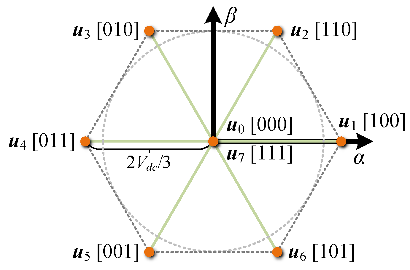
2.1. Mathematic Model

At present, the power conversion system of wind power generation is normally designed as a cascaded construction, i.e., the so-called back-to-back converter [4], which consists of a two-level AC/DC converter on the machine side, a two-level DC/AC converter on the grid side and a decoupling capacitor between them. The AC/DC and DC/AC converters can be controlled separately, and their control methods are very similar. In this paper, the AC/DC converter of a direct-driven wind power generation system is investigated, and its topology is presented in Figure 1 [4], where V_dc is the DC-link voltage and i_a, i_b and i_c are the three-phase stator currents, respectively, and w_m refers to the mechanical angular speed of the blade.

Before designing a control method, the mathematical model of the system under test must be constructed carefully [24]. The modeling process should start with an analysis of the circuit by obtaining a set of differential equations [25,26]. Regarding power conversion systems, the dq frame is always selected, from which the mathematical model of the converter shown in Figure 1 can be described using a state space equation as follows:

$$\dot{x}=Ax+Bu+C$$

(1)

with

$$x={\left[\begin{array}{cc}{i}_d& i_q\end{array}\right]}^T,u={\left[\begin{array}{cc}{u}_d& u_q\end{array}\right]}^T$$

(2)

$$A=\left[\begin{array}{cc}-{\displaystyle \frac{R_s}{L_d}}& -{\displaystyle \frac{{\omega }_e{L}_q}{L_d}}\\ {\displaystyle \frac{{\omega }_e{L}_d}{L_q}}& -{\displaystyle \frac{R_s}{L_q}}\end{array}\right],B=\left[\begin{array}{cc}-{\displaystyle \frac{1}{L_d}}& 0\\ 0& -{\displaystyle \frac{1}{L_q}}\end{array}\right],C=\left[\begin{array}{l}0\\ {\displaystyle \frac{{\omega }_e{\psi }_f}{L_q}}\end{array}\right]$$

(3)

where i_d and i_q are the dq-axis components of stator currents; u_d and u_q are the dq-axis components of voltages determined by the switching state of the converter; L_d and L_q are the dq-axis stator inductances; R_s is the stator resistance; and ω_e and ψ_f are the electrical angular speed and the PM flux, respectively.

The input variable u = [u_d u_q]^T is regulated by the converter switching state and DC-link voltage V_dc, expressed as follows:

$$\left[\begin{array}{l}{u}_d\\ u_q\end{array}\right]=T_{abc/dq}\left[\begin{array}{l}{u}_{aN}\\ u_{bN}\\ u_{cN}\end{array}\right]={\displaystyle \frac{V_{dc}}{3}}\cdot T_{abc/dq}\left[\begin{array}{l}2S_a-S_b-S_c\\ 2S_b-S_a-S_c\\ 2S_c-S_a-S_b\end{array}\right]$$

(4)

with the transformation matrix T_abc/dq written as [13]

$$T_{abc/dq}={\displaystyle \frac{2}{3}}\left[\begin{array}{ccc}\cos {\theta }_e& \cos \left({\theta }_e-2\pi /3\right)& \cos \left({\theta }_e+2\pi /3\right)\\ -\sin {\theta }_e& -\sin \left({\theta }_e-2\pi /3\right)& -\sin \left({\theta }_e+2\pi /3\right)\end{array}\right]$$

(5)

where u_aN, u_bN, and u_cN are the voltages of three-phase leg mid-points a, b, and c with respect to the neutral point of stator windings, N, respectively, as seen in Figure 1; S_a, S_b, and S_c show the operating situations of the three-phase legs; and θ_e denotes the electrical angle of the rotor.

The two switches of each phase are conducted alternatively, and S_x (x = a, b, and c) is either 1 or 0, indicating that the upper or the lower switch is ON. The combination of operating situations of three-phase legs leads to eight possible converter switching states, expressed by [S_a S_b S_c]. Each one corresponds to a voltage vector, as shown in Figure 2 [8]. The six active voltage vectors (u₁–u₆) graphically describe a hexagon that has a magnitude of 2 V_dc/3, while the two zero voltage vectors (u₀ and u₇) are at the origin. The core of modern control methods lies in the manipulation of these voltage vectors.

2.2. Principle and Implementation of Basic FS-ULMPCC Method

In addition to the prediction model, the basic FS-ULMPCC method is the same as the FS-MPCC method. The implementation of the basic FS-ULMPCC method consists of the following three steps [6]: (1) forecasting the future dq-axis currents for all accessible voltage vectors (see Figure 2) based on a prediction model (e.g., x(k + 1) = f[x(k), u_i], where ‘k’ and ‘k + 1′ denote the kth and (k + 1)th sampling period, respectively), (2) evaluating the voltage vectors with a cost function (e.g., g(u_i) = |x* − x(k + 1|u_i)${|}_2^2$, where x* denotes the reference of x; (3) seeking out the optimal voltage vector by means of an optimization scheme. It is clear that the prediction model, cost function, and optimization scheme are three crucial elements to be considered in the basic FS-ULMPCC, as detailed in the following subsections.

2.2.1. Prediction Model

The difference between FS-ULMPCC and FS-MPCC is mainly due to the prediction model. In the traditional FS-MPCC method, the prediction model is the discretized form of mathematical model (1), as shown below [7]:

$$x\left(k+1\right)=x\left(k\right)+T_s\left[Ax\left(k\right)+Bu\left(k\right)+C\right]$$

(6)

From this, it is certain that machine parameters are involved in the prediction model, and thus, parameter mismatches must result in prediction errors.

In the FS-ULMPCC method, the mathematical model is replaced by ULM, which removes the machine parameters [14]. The ULM corresponding to (1) can be written as follows:

$$\dot{x}=\alpha u+F$$

(7)

where α is a two-dimension coefficient matrix, which, in principle, is equal to the matrix B in (1), while rough knowledge of B is enough when designing α [15]; F refers to the term of lumped disturbance, describing all parameter-related and unknown portions in the original mathematical model [13].

By discretizing (7), the prediction model adopted in the FS-ULMPCC method can be obtained as follows:

$$x\left(k+1\right)=x\left(k\right)+T_s\left[F+\alpha u\left(k\right)\right]$$

(8)

The estimation of F is undoubtedly essential to the FS-ULMPCC method, which can be carried out using state observers, such as LESO [14], SMO [16], and LO [18]. Comparatively, LESO is simpler than SMO and LO in terms of digital implementation. Therefore, an LESO was designed in this study to estimate the lumped disturbance F, as follows [14]:

$$\{\begin{array}{l}{e}_{rr}=z_1-x\\ {\dot{z}}_1=z_2+\alpha u-{\beta }_1{e}_{rr}\\ {\dot{z}}_2=-{\beta }_2{e}_{rr}\end{array}$$

(9)

where z₁ is the estimated value of x; e_rr is the error between the estimated and actual values of x; z₂ is the estimated value of F; β₁ = 2ω₀, β₂ = ω₀² are the only two coefficients to be chosen in an LESO [14]; and ω₀ is determined by the control frequency. Thus, the prediction model in (8) can be rewritten as follows:

$$x\left(k+1\right)=x\left(k\right)+T_s\left[\widehat{F}+\alpha u\right]$$

(10)

where the cap ‘ˆ’ denotes the estimated value.

2.2.2. Cost Function

The cost function is normally defined as the 2-norm of the current tracking errors:

$$g\left(u_i\right)={\Vert x^{*}-x\left(k+1|u_i\right)\Vert }_2^2$$

(11)

Likewise, 1-norm of the current tracking errors is also applicable. Nonetheless, it is verified that the use of 2-norm is more advantageous to the system’s stability [27].

2.2.3. Optimization Scheme

For two-level converters, the enumeration scheme is always applied to select the optimal voltage vector [13]. The optimal input corresponds to the minimum value of the cost function, which can be determined by the following:

$$u_{opt}=\underset{u_i\in \nu }{\arg \min }g\left(u_i\right)$$

(12)

where v refers to the control set that is composed of the possible voltage vectors as in Figure 2, i.e., v = {u₁, u₂, …, u₇}. In the case of a large number of possible choices (e.g., multi-level or multi-phase converters), more efficient optimization schemes are preferred.

3. Proposed FS-ULMPCC Method

In this paper, a novel FS-ULMPCC is proposed for the AC/DC converter of direct-driven wind power generation. The overall control diagram is presented in Figure 3. A PI controller is adopted in the outer loop of the voltage regulator. In the inner loop of current control, the control set is reconstructed according to the deadbeat concept, followed by current prediction, cost function evaluation, optimal option selection, and duty cycle allocation. These modules are explained in the following figure.

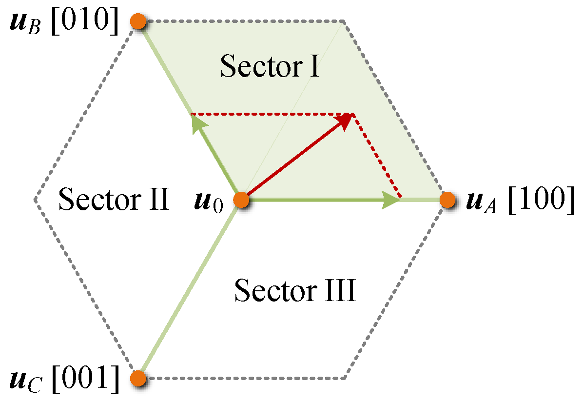
3.1. Reconstruction of Control Set

Normally, six active voltage vectors divide the αβ frame into six sectors, as shown in Figure 2. Of the six vectors, u₁, u₃, and u₅ correspond to switching states 100, 010, and 001, respectively. These switching states generate voltages applied to three-phase stators independently so that a combination of them satisfies the superposition principle. Thus, the three vectors are considered to reconstruct the control set, renamed as u_A, u_B, and u_C, respectively. Meanwhile, the three vectors split the αβ frame into three parallelogram-shaped regions, as shown in Figure 4, i.e., Sector I, Sector II, and Sector III.

On the basis of vector addition law, for example, any voltage vector located in sector I can be formed by u_A and u_B with positive weights. For voltage vectors lying in other sectors, the two vectors used for formulation alter accordingly, which are counted as u_x and u_y, respectively, as summarized in

Table 1. Vectors for formulation in different sectors.

Sector	ux	uy
I	uA	uB
II	uB	uC
III	uC	uA

.

According to the deadbeat concept, the voltage vector leading to zero current tracking errors can be seen as the desired voltage vector (tagged with u_ref). This implies that the cost function value corresponding to u_ref is equal to 0 [namely x(k + 1) = x*]. Considering a pair of voltage vectors in Table 1, u_ref can be synthesized using

$$u_{ref}=d_x{u}_x+d_y{u}_y$$

(13)

where d_x and d_y are the duty cycles of u_x and u_y, respectively. The dq-axis components of u_ref can be calculated by

$$\{\begin{array}{l}{u}_{ref\_d}=d_x{u}_{xd}+d_y{u}_{yd}\\ u_{ref\_q}=d_x{u}_{xq}+d_y{u}_{yq}\end{array}$$

(14)

where u_{ref_d} and u_{ref_q} are the dq-axis components of u_ref, respectively; u_xd and u_xq are the dq-axis components of u_x, respectively; and u_yd and u_yq are the dq-axis components of u_y, respectively.

Letting x(k + 1) = x* for the sake of deadbeat control and substituting (14) into (10), the duty cycles of u_x and u_y can be solved as follows:

$$\{\begin{array}{l}{d}_y={\displaystyle \frac{u_{xq}\left({\delta }_d+{\sigma }_d\right)-u_{xd}\left({\delta }_q+{\sigma }_q\right)}{u_{xq}{u}_{yd}-u_{xd}{u}_{yq}}}\\ d_x={\displaystyle \frac{{\delta }_d+{\sigma }_d-u_{yd}{d}_y}{u_{xd}}}\end{array}$$

(15)

with

$$\{\begin{array}{l}{\delta }_d={\displaystyle \frac{i_d^{*}-i_d\left(k\right)}{{\alpha }_d{T}_s}}\\ {\delta }_q={\displaystyle \frac{i_q^{*}-i_q\left(k\right)}{{\alpha }_q{T}_s}}\\ {\sigma }_d=-{\displaystyle \frac{F_d}{{\alpha }_d}}\\ {\sigma }_q=-{\displaystyle \frac{F_q}{{\alpha }_q}}\end{array}$$

(16)

Note that each pair of voltage vectors in Table 1 corresponds to a set of solutions (d_x, d_y). As such, three elements should be embraced in the reconstructed control set v_prop, which can be expressed as follows:

$$v_{\mathrm{prop}}=\left\{\left\{u_{x1},u_{y1},d_{x1},d_{y1}\right\},\left\{u_{x2},u_{y2},d_{x2},d_{y2}\right\},\left\{u_{x3},u_{y3},d_{x3},d_{y3}\right\}\right\}$$

(17)

3.2. Current Prediction

The current predictions should be conducted for each choice of v_prop, following the prediction model shown in (10). The prediction model can be rewritten as follows:

$$x\left(k+1|\left\{u_{xj},u_{yj},d_{xj},d_{yj}\right\}\right)=x\left(k\right)+T_s\left[\widehat{F}+\alpha u\left(k|\left\{u_{xj},u_{yj},d_{xj},d_{yj}\right\}\right)\right]$$

(18)

In addition, implicit constraints on duty cycles d_x and d_y must be taken into account. On one hand, it is mandatory that the duty cycles must be non-negative; namely, the lower limit of d_x and d_y should be 0. On the other hand, the upper limit of d_x and d_y should be one. When d_x or d_y is larger than one, the other value should be decreased accordingly to ensure the direction of the synthesized voltage vector. Considering this, the calculated values of d_x and d_y should be corrected as follows:

$$\{\begin{array}{l}{d}_{xj}=0,d_{xj}<0\\ d_{yj}=0,d_{yj}<0\end{array}$$

(19)

$$\{\begin{array}{l}\{\begin{array}{l}{d}_{xj}=d_{xj}/d_{yj}\\ d_{yj}=1\end{array},d_{yj}>1\mathrm{and}{d}_{yj}>d_{xj}\\ \{\begin{array}{l}{d}_{xj}=1\\ d_{yj}=d_{yj}/d_{xj}\end{array},d_{xj}>1\mathrm{and}{d}_{xj}>d_{yj}\end{array}$$

(20)

3.3. Cost Function Evaluation and Optimal Option Selection

In this step, each element in v_prop should be assessed by the cost function in (11). In accordance with (18), the cost function in (11) and the optimal option in (12) can be rewritten as follows:

$$g\left(\left\{u_{xj},u_{yj},d_{xj},d_{yj}\right\}\right)={\Vert x^{*}-x\left(k+1|\left\{u_{xj},u_{yj},d_{xj},d_{yj}\right\}\right)\Vert }_2^2$$

(21)

$$\left\{u_{xopt},u_{yopt},d_{xopt},d_{yopt}\right\}=\underset{\left\{u_{xj},u_{yj},d_{xj},d_{yj}\right\}\in {\nu }_{\mathrm{prop}}}{\arg \min g\left(\left\{u_{xj},u_{yj},d_{xj},d_{yj}\right\}\right)}$$

(22)

3.4. Duty Cycle Allocation

On the foundation of {u_xopt, u_yopt, d_xopt, and d_yopt}, the duty cycles of three-phase legs can be further allocated. The reconstructed control set based on three independent voltage vectors (u_A, u_B, and u_C) extremely simplifies the allocation. The calculated duty cycles can be directly applied to the corresponding phase legs. For example, in the case of u_xopt = u_A, u_yopt = u_B when d_xopt > d_yopt, the duty cycles of three-phase legs can be expressed as follows:

$$\{\begin{array}{l}{d}_A=d_{xopt}\\ d_B=d_{yopt}\\ d_C=0\end{array}$$

(23)

However, such an allocation leads to the phenomenon of an unfixed switching frequency, as one leg keeps its state at each control period. This operation causes side effects on the system [20]. In order to tackle this issue, the fashion of signal generation in SVPMM is adopted (i.e., the so-called seven-segment pulse sequence). The two zero voltage vectors are applied together with the active ones. The duty cycle of zero voltage vectors can be calculated as follows:

$$d_0=\{\begin{array}{l}1-d_{xopt},d_{xopt}\ge d_{yopt}\\ 1-d_{yopt},d_{xopt}<d_{yopt}\end{array}$$

(24)

By equally assigning d₀ to u₀[000] and u₇[000], the duty cycles of the three-phase legs shown (23) should be corrected as follows:

$$\{\begin{array}{l}{d}_A=d_{xopt}+{\displaystyle \frac{d_0}{2}}\\ d_B=d_{yopt}+{\displaystyle \frac{d_0}{2}}\\ d_C={\displaystyle \frac{d_0}{2}}\end{array}$$

(25)

The control signals corresponding to (23) and (25) are drawn in Figure 5. Other cases can be analyzed similarly.

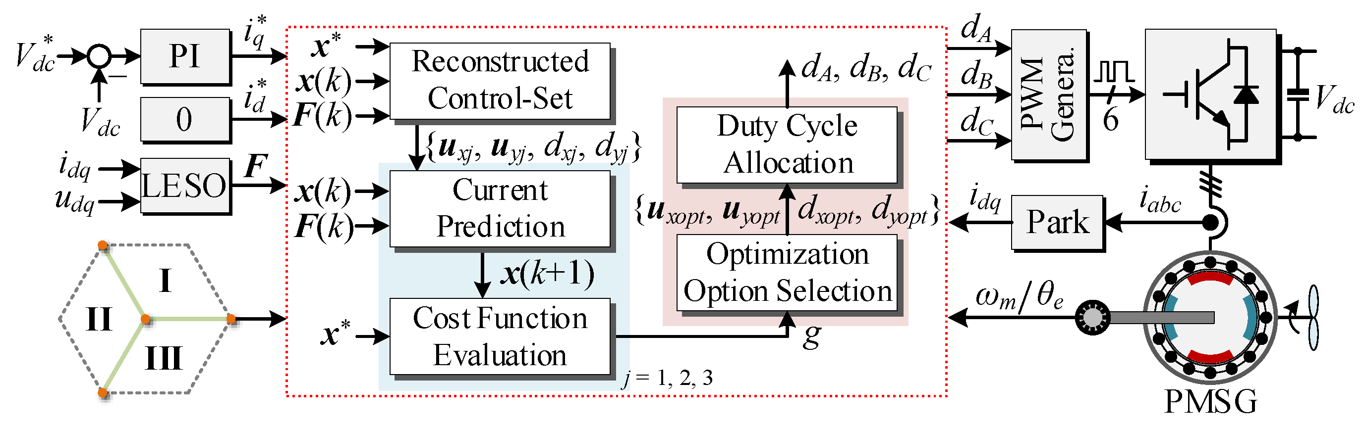
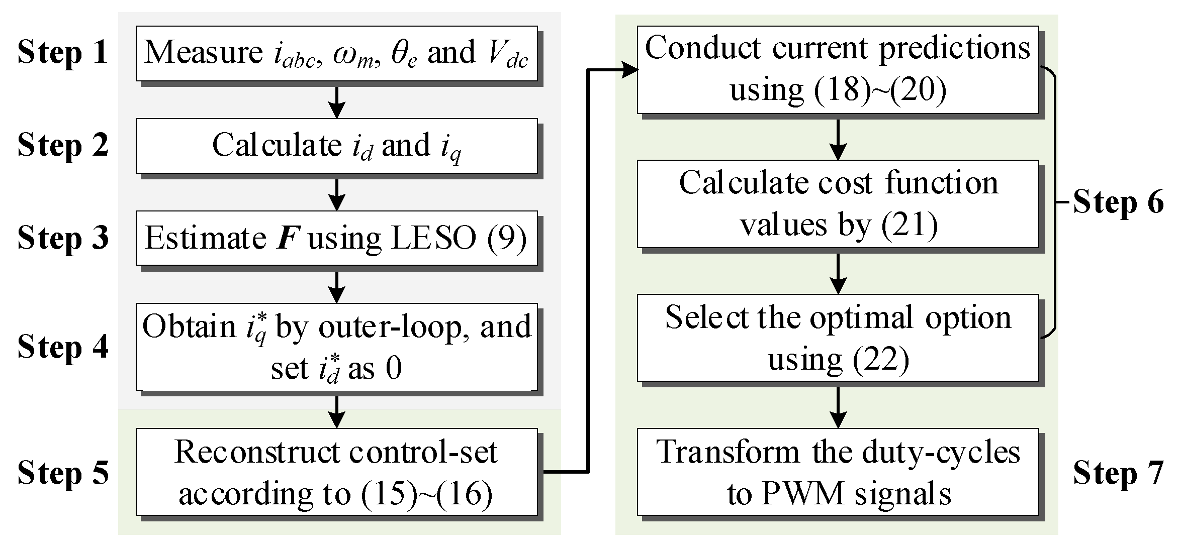
3.5. Summary of the Proposed FS-ULMPCC Method

An implementation flow chart of the proposed FS-ULMPCC is presented in Figure 6. The following seven steps should be implemented.

• Step 1: Measure the information of the stator currents (i_a, i_b, and i_c), machine speed (ω_m), rotor electrical angle (θ_e), and DC-link voltage (V_dc).
• Step 2: Calculate the dq-axis currents (i_d and i_q) using Park’s transformation.
• Step 3: Estimate the lumped disturbance (F) using the LESO seen in (9).
• Step 4: Obtain the q-axis current reference (i_q*) using the outer voltage controller and set the d-axis current reference (i_d*) to 0.
• Step 5: Reconstruct the control set v_prop according to (15) and (16).
• Step 6: Conduct the current predictions in (18)–(20), calculate the cost function values using (21), and select the optimal choice using (22).
• Step 7: Transform the duty cycles to PWM signals for the three-phase legs of the converter.

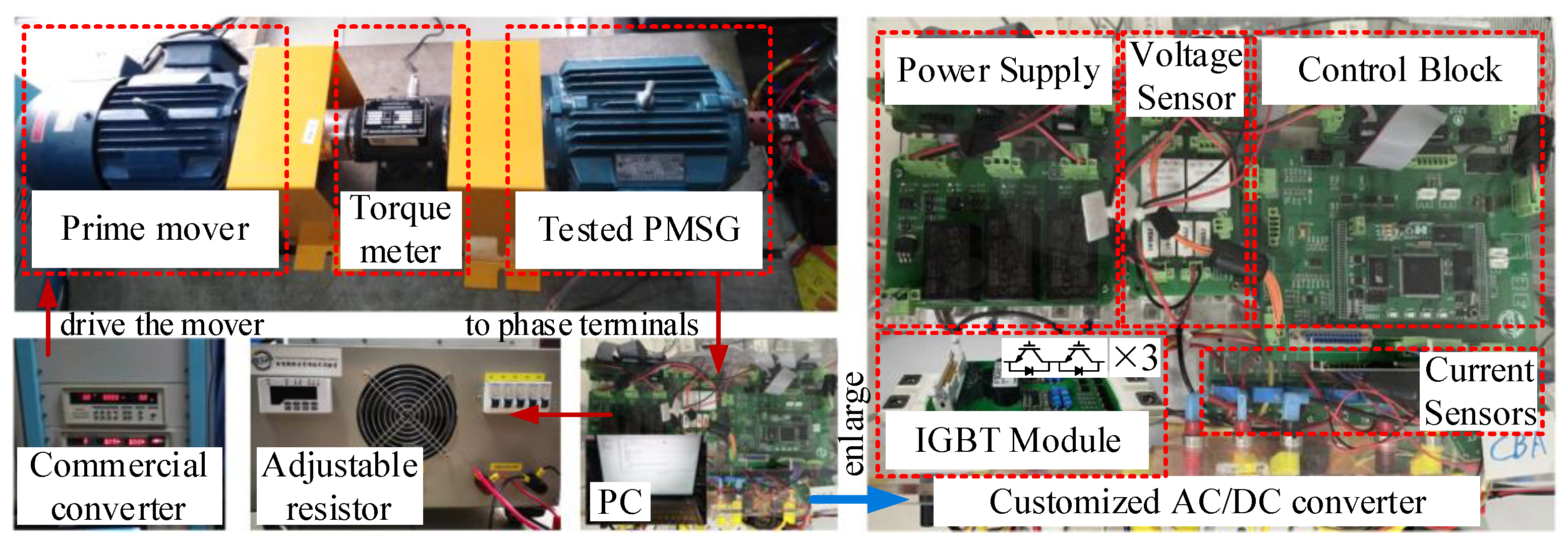
4. Experimental Verification

4.1. Experimental Test Rig

In order to verify the effectiveness of the proposed method, numerous experiments were conducted based on a 2 kW proof-of-concept test rig, as shown in Figure 7. The main parameters of the PMSG under test are given in

Table 2. Main parameters of the PMSG under test.

Symbol	Quantity	Value
PN	Rated power	2.2 kW
nN	Rated speed	800 rpm
np	Pole pairs	2
Rs	Stator resistance	5.25 Ω
Ld	d-axis inductance	24 mH
Lq	q-axis inductance	36 mH
ψf	PM flux	0.8 Wb

. An induction machine driven by a commercial variable-frequency converter was employed to simulate the prime mover. The customized AC/DC converter is composed of three insulated-gate bipolar transistor (IGBT) modules (FF300R12ME4, from Infineon, Munich, Germany). In the DC-link of the converter, there is a 470 μF/450 V aluminum electrolytic capacitor connected in parallel with an adjustable resistor, which serves as the load to expend the generated power. The machine rotor’s position, machine currents, and DC-link voltage are measured using an encoder (E6B2-CWZ3E, from OMRON, Kyoto, Japan), three current sensors (HAS 50-S, from LEM, Geneva, Switzerland), and a voltage sensor (LV25-P, from LEM, Geneva, Switzerland), respectively. All sensed signals are fed into a digital signal processor (TMS320F28335, from TI, Dallas, TX, United States), and the real-time programs are developed in C language on Code Composer Studio 7.4.0 software. In addition to the proposed method, a traditional version of the FS-ULMPCC method is also tested for comparison, as explained in Section 2. For both methods, the sampling frequency, as well as the control frequency, is set to 10 kHz. The coefficients involved in these two methods are summarized in

Table 3. Coefficients involved in tested methods.

Symbol	Description	Value
Kp	Proportional coefficient of voltage regulator	0.02
Ki	Integral coefficient of voltage regulator	5
α	Coefficient matrix in prediction model (10)	[40 0; 0 30]
ω0	Coefficient involved in LESO (9)	2000

.

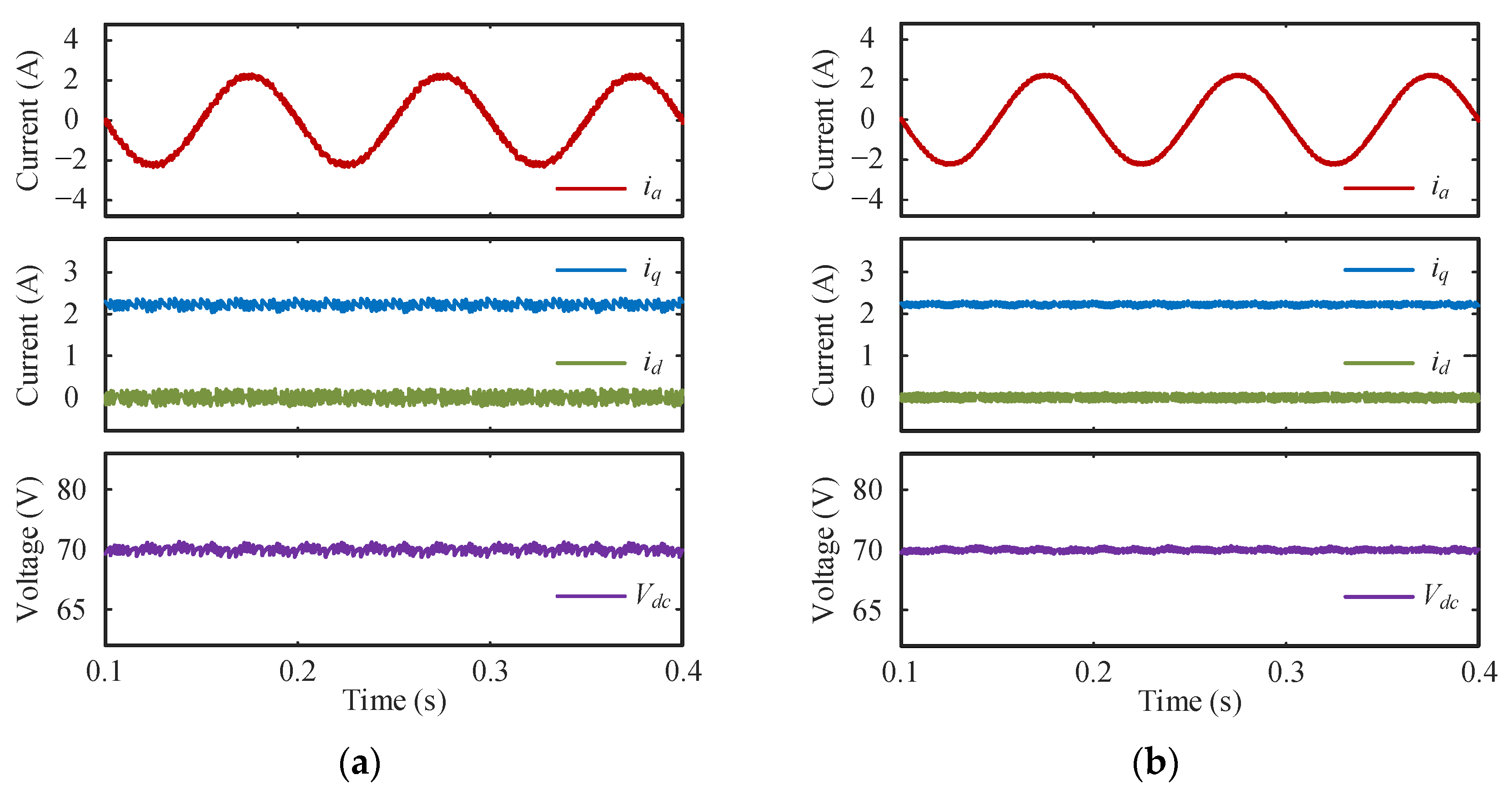
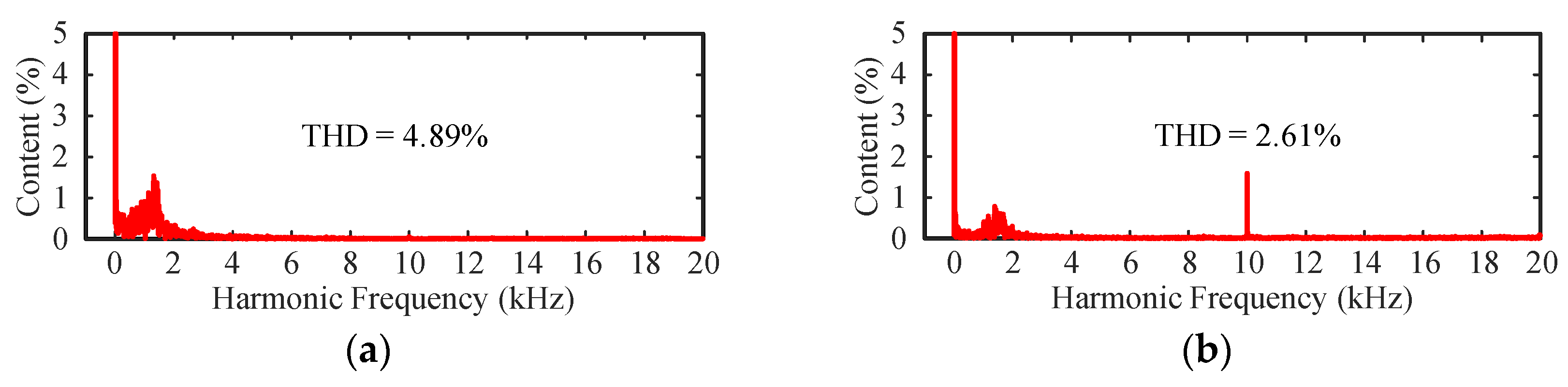
4.2. Steady-State Performance Comparison

First, these two methods are compared in terms of steady-state performance in a manner where the speed of the prime mover is set to 300 rpm, the DC-link voltage reference is set to 70 V, and the load resistor is adjusted to 40 Ω. The results of the stator current (i_a), dq-axis components of stator currents (i_d and i_q), and DC-link voltage (V_dc) are shown in Figure 8. As seen, both methods can yield a sinusoidal stator current and regulate the dq-axes currents and DC-link voltage to track their demands. The waveforms show that the steady-state performance of the proposed method is evidently superior to the traditional method.

The fast Fourier transform (FFT) analysis results of stator currents are given in Figure 9, which shows the harmonic spectrums and total harmonic distortion (THD) values of stator currents controlled by two methods. Compared to the traditional method, the proposed FS-ULMPCC can greatly reduce the THD values from 4.89% to 2.61%. Meanwhile, two differences between the two spectrums can be observed, firmly indicating the advantages of the proposed method. On one hand, low harmonic contents can be weakened to a large extent using the proposed method. On the other hand, the harmonic contents around the control frequency (10 kHz) are particularly prominent, which implies that the switching frequency of the converter under the control of the proposed method is constant.

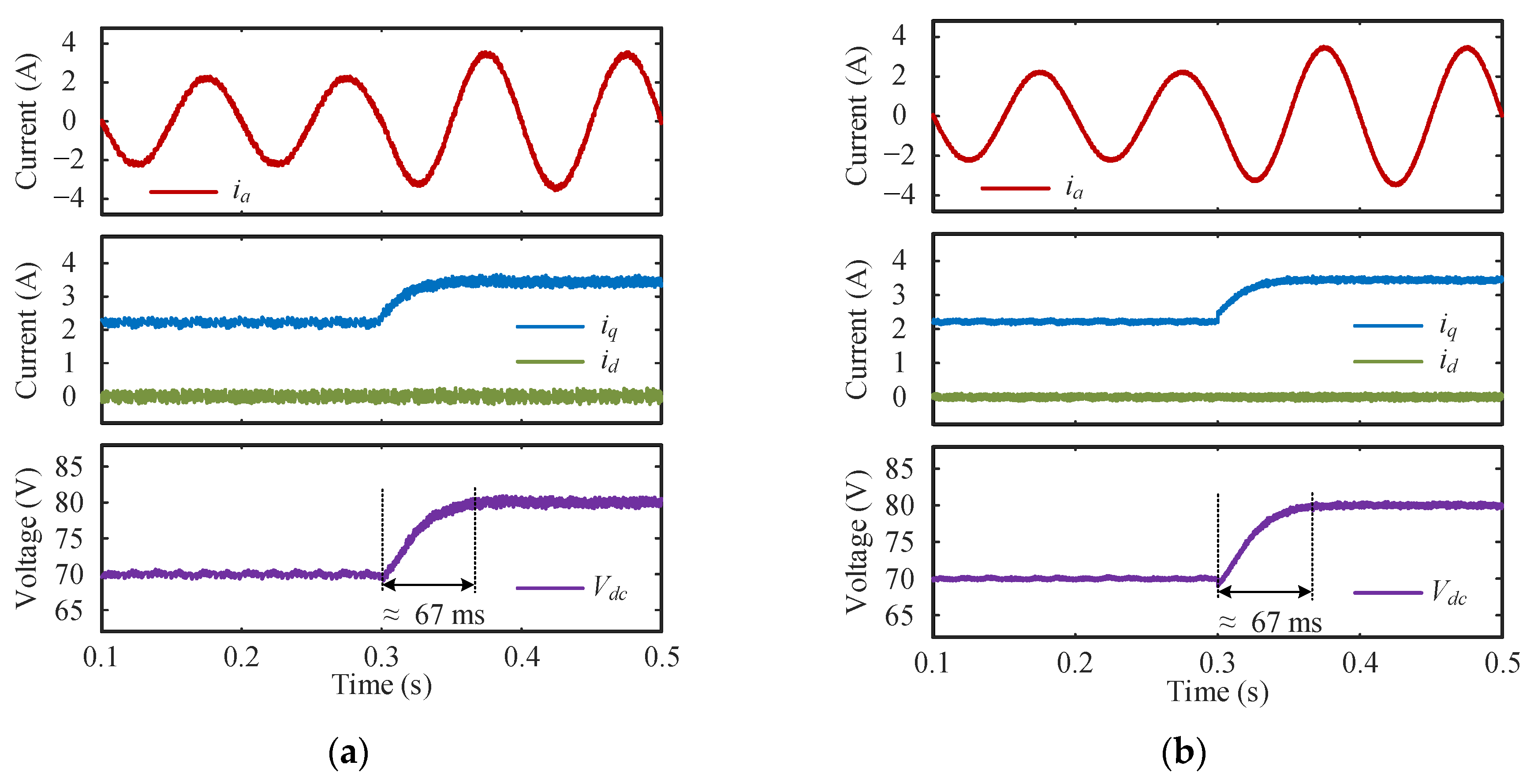
4.3. Transient Performance Comparison

Thereafter, the transient performance of the two methods is evaluated and compared. The results given in Figure 10 follow an initial load resistor of 40 Ω with a sudden change to 30 Ω. As seen, smooth voltage curves without overshoots are obtained in both methods. The response processes are nearly the same, and the response time is roughly 75 ms. The voltage drops are less than 5 V in both methods. The results of the transient experiments in response to the voltage reference changing from 70 V to 80 V are presented in Figure 11. As observed, the DC-link voltage curves are also very smooth, and no overshoots exist. The duration of transients is nearly the same as well, lasting about 67 ms. In summary, the tests demonstrate the good transient performance of the proposed method.

4.4. Computational Burden Evaluation

Finally, the computational burden of the two methods is evaluated. For this purpose, the clock cycles required for codes to be implemented are measured in such a way that two breakpoints are set at the beginning and end of the interruptions triggered once per control period. The results are concluded in

Table 4. Computational burden comparison.

	Clock Cycles	Execution Time
Traditional FS-ULMPCC method	5384	35.89 μs
Proposed FS-ULMPCC method	4685	31.23 μs

. As seen, 5384 and 4685 clock cycles, corresponding approximately to 35.89 μs and 31.23 μs, are needed for the implementation of the two methods, respectively. Comparatively, the proposed method is more efficient than the traditional one because only three elements are included in the reconstructed control set. The reduction in execution time (approximately 4.66 μs) is relatively limited. The reason for this is that the calculation of the reconstructed control set involves a host of multiplication and division operations.

5. Conclusions

In this paper, a novel FS-ULMPCC method with enhanced steady-state performance is proposed, which is designed based on LESO and applied to the AC/DC converter of a direct-driven wind power generation system. A new control set reconstruction strategy is proposed by which only three options are included in the control set for optimization. Each option is associated with two independent, active voltage vectors and their durations. Through experiments, the effectiveness of the proposed FS-ULMPCC is demonstrated. From the obtained results, the following conclusions can be extracted:

(1)

In terms of steady-state performance, the proposed FS-ULMPCC method is evidently superior to the traditional one. Not only can the current THD value be reduced from 4.89% to 2.61% but also the inverter operation with a constant switching frequency can also be realized.

(2)

In terms of transient performance, the proposed FS-ULMPCC method is considerable to a traditional one in response to both load change and voltage reference alternation cases. The obtained voltage curves are very smooth without any overshoots, and the transients last less than 80 ms.

(3)

In terms of computational burden, the proposed FS-ULMPCC method is more efficient than the traditional one, thanks to the fact that only three options are embraced in the reconstructed control set. The reduction in execution time is approximately 4.66 μs.

Despite the aforementioned merits, a potential drawback of the proposed method is that the design of the coefficient matrix in the prediction model still requires rough knowledge of the inductance values of machines. Our future work will focus on the adaptive tuning scheme of the coefficient matrix. In addition, the proposed strategy needs mathematical simplification for the implementation process in order to further reduce the computational burden.

References

1. Li, B.; Fesseha, S.B.; Chen, S.; Zhou, Y. Real-time solar power generation scheduling for maintenance and suboptimally performing equipment using demand response unified with model predictive control. Energies 2024, 17, 3212. [Google Scholar] [CrossRef]
2. Boland, J. Constructing interval forecasts for solar and wind energy using quantile regression, ARCH and exponential smoothing methods. Energies 2024, 17, 3240. [Google Scholar] [CrossRef]
3. Wang, Y.; Meng, J.H.; Zhang, X.Y.; Xu, L. Control of PMSG-based wind turbines for system inertial response and power oscillation damping. IEEE Trans. Sustain. Energy 2015, 6, 565–574. [Google Scholar] [CrossRef]
4. Wu, M.Z.; Ding, L.; Xu, X.N.; Wang, K.; Lu, Q.W.; Li, Y.W. A common-mode voltage elimination scheme by reference voltage decomposition for back-to-back two-level converters. IEEE Trans. Ind. Electron. 2024, 71, 4463–4473. [Google Scholar] [CrossRef]
5. Xu, X.N.; Wu, M.Z.; Wang, K.; Zheng, Z.D.; Deng, Z.F.; Li, Y.W.; Li, Y.D. A simple method for common-mode voltage reduction and neutral-point potential balance of back-to-back three-level NPC converters. IEEE J. Emerg. Sel. Top. Power Electron. 2024, 12, 2855–2869. [Google Scholar] [CrossRef]
6. Rodriguez, J.; Garcia, C.; Mora, A.; Flores-Bahamonde, F.; Acuna, P.; Novak, M.; Zhang, Y.; Tarisciotti, L.; Davari, S.A.; Zhang, Z.; et al. Latest advances of model predictive control in electrical drives—Part I: Basic concepts and advanced strategies. IEEE Trans. Power Electron. 2022, 37, 3927–3942. [Google Scholar] [CrossRef]
7. Rodriguez, J.; Valencia, D.F.; Elmorshedy, M.; Wang, F.; Zuo, K.; Tarisciotti, L.; Flores-Bahamonde, F.; Xu, W.; Zhang, Z.; Zhang, Y.; et al. Latest advances of model predictive control in electrical drives—Part II: Applications and benchmarking with classical control methods. IEEE Trans. Power Electron. 2022, 37, 5047–5061. [Google Scholar] [CrossRef]
8. Zhang, Y.C.; Xia, B.; Yang, H.T.; Rodriguez, J. Overview of model predictive control for induction motor drives. Chin. J. Electr. Eng. 2016, 2, 62–76. [Google Scholar]
9. Zhang, X.G.; Zhang, L.; Zhang, Y.C. Model predictive current control for PMSM drives with parameter robustness improvement. IEEE Trans. Power Electron. 2019, 34, 1645–1657. [Google Scholar] [CrossRef]
10. Chen, Z.; Qiu, J.; Jin, M. Adaptive finite-control-set model predictive current control for IPMSM drives with inductance variation. IET Electr. Power Appl. 2017, 11, 874–884. [Google Scholar] [CrossRef]
11. Guo, L.; Xu, Z.; Li, Y. An inductance online identification-based model predictive control method for grid-connected inverters with an improved phase-locked loop. IEEE Trans. Transp. Electrif. 2022, 8, 2695–2709. [Google Scholar] [CrossRef]
12. Lin, C.; Liu, T.; Yu, J. Model-free predictive current control for interior permanent-magnet synchronous motor drives based on current difference detection technique. IEEE Trans. Ind. Electron. 2014, 61, 667–681. [Google Scholar] [CrossRef]
13. Liu, X.; Yang, H.; Lin, H.Y.; Yu, F.; Yang, Y. A novel finite-set sliding-mode model-free predictive current control for PMSM drives without dc-link voltage sensor. IEEE Trans. Power Electron. 2024, 39, 320–331. [Google Scholar] [CrossRef]
14. Zhang, Y.C.; Jin, J.; Huang, L. Model-free predictive current control of PMSM drives based on extended state observer using ultralocal model. IEEE Trans. Ind. Electron. 2021, 68, 993–1003. [Google Scholar] [CrossRef]
15. Fliess, M.; Join, C. Model-free control. Int. J. Control 2013, 86, 2228–2252. [Google Scholar] [CrossRef]
16. Sun, Z.; Deng, Y.; Wang, J. Finite control set model-free predictive current control of PMSM with two voltage vectors based on ultralocal model. IEEE Trans. Power Electron. 2023, 38, 776–788. [Google Scholar] [CrossRef]
17. Mousavi, M.S.; Davari, S.A.; Nekoukar, V. Integral sliding mode observer-based ultralocal model for finite-set model predictive current control of induction motor. IEEE J. Emerg. Sel. Top. Power Electron. 2022, 10, 2912–2922. [Google Scholar] [CrossRef]
18. Yang, N.; Zhang, S.; Li, X. A new model-free deadbeat predictive current control for PMSM using parameter-free Luenberger disturbance observer. IEEE J. Emerg. Sel. Top. Power Electron. 2023, 11, 407–417. [Google Scholar] [CrossRef]
19. Luo, Y.; Liu, C. Model predictive control for a six-phase PMSM motor with a reduced-dimension cost function. IEEE Trans. Ind. Electron. 2020, 67, 969–979. [Google Scholar] [CrossRef]
20. Xia, L.; Xu, L.; Yang, Q.; Yu, F.; Zhang, S. An MPC scheme with enhanced active voltage vector region for V2G inverter. Energies 2020, 13, 1312. [Google Scholar] [CrossRef]
21. Zhang, Y.; Yang, H. Two-vector-based model predictive torque control without weighting factors for induction motor drives. IEEE Trans. Power Electron. 2016, 31, 1381–1390. [Google Scholar] [CrossRef]
22. Sun, X.; Li, T.; Yao, M.; Lei, G.; Guo, Y.; Zhu, J. Improved finite-control-set model predictive control with virtual vectors for PMSHM drives. IEEE Trans. Energy Convers. 2022, 37, 1885–1894. [Google Scholar] [CrossRef]
23. Gu, M.; Yang, Y.; Fan, M.D.; Xiao, Y.; Liu, P.; Zhang, X.N.; Yang, H.; Rodriguez, J. Finite control set model predictive torque control with reduced computation burden for PMSM based on discrete space vector modulation. IEEE Trans. Energy Convers. 2023, 38, 703–712. [Google Scholar] [CrossRef]
24. Djellab, N.; Boureghda, A. A moving boundary model for oxygen diffusion in a sick cell. Comput. Methods Biomech. Biomed. 2021, 25, 1402–1408. [Google Scholar] [CrossRef] [PubMed]
25. Boureghda, A.; Djellab, N. Du fort-frankel finite difference scheme for solving of oxygen diffusion problem inside one cell. J. Comput. Theor. Transp. 2023, 52, 363–373. [Google Scholar] [CrossRef]
26. Boureghda, A. Solution to an ice melting cylindrical problem. J. Nonlinear Sci. Appl. 2016, 9, 1440–1452. [Google Scholar] [CrossRef]
27. Karamanakos, P.; Geyer, T. Guidelines for the design of finite control set model predictive controllers. IEEE Trans. Power Electron. 2020, 35, 7434–7450. [Google Scholar] [CrossRef]
Figure 1. Topology of the AC/DC converter for a direct-driven wind power generation system.
Electronics 13 03302 g001
Figure 2. Relationship between voltage vectors and converter-switching states.
Electronics 13 03302 g002
Figure 3. Overall control diagram of the proposed FS-ULMPCC method.
Electronics 13 03302 g003
Figure 4. Three independent voltage vectors used for reconstruction of control set.
Electronics 13 03302 g004
Figure 5. Control signals of three-phase legs without correction in (a) and with correction in (b) for the cases of uxopt = uA, uyopt = uB, and dxopt > dyopt.
Electronics 13 03302 g005
Figure 6. Implementation flow chart of the proposed FS-ULMPCC.
Electronics 13 03302 g006
Figure 7. Experimental proof-of-concept test rig.
Electronics 13 03302 g007
Figure 8. Steady-state performance of (a) traditional FS-ULMPCC and (b) proposed FS-ULMPCC in case of that the speed of prime mover is set to 300 rpm and the DC-link voltage reference is set to 70 V.
Electronics 13 03302 g008
Figure 9. Total harmonic distortion values obtained by fast Fourier transform (FFT) analysis of (a) traditional FS-ULMPCC and (b) proposed FS-ULMPCC.
Electronics 13 03302 g009
Figure 10. Transient performance of (a) traditional FS-ULMPCC and (b) proposed FS-ULMPCC in response to the load change from 40 Ω to 30 Ω.
Electronics 13 03302 g010
Figure 11. Transient performance of (a) traditional FS-ULMPCC and (b) proposed FS-ULMPCC in response to the voltage reference change from 70 V to 80 V.
Electronics 13 03302 g011