Abstract
Depth image has been widely involved in various tasks of 3D systems with the advancement of depth acquisition sensors in recent years. Depth images suffer from serious distortions near object boundaries due to the limitations of depth sensors or estimation methods. In this paper, a simple method is proposed to rectify the erroneous object boundaries of depth images with the guidance of reference RGB images. First, an RGB–Depth boundary inconsistency model is developed to measure whether collocated pixels in depth and RGB images belong to the same object. The model extracts the structures of RGB and depth images, respectively, by Gaussian functions. The inconsistency of two collocated pixels is then statistically determined inside large-sized local windows. In this way, pixels near object boundaries of depth images are identified to be erroneous when they are inconsistent with collocated ones in RGB images. Second, a depth image rectification method is proposed by embedding the model into a simple weighted mean filter (WMF). Experiment results on two datasets verify that the proposed method well improves the RMSE and SSIM of depth images by 2.556 and 0.028, respectively, compared with recent optimization-based and learning-based methods.
1. Introduction
Depth image usage has been involved in various tasks of 3D systems with the advances in depth acquisition sensors in recent years, such as in 3D reconstruction, SLAM, and so on. A depth image is generally acquired together with a reference RGB image. It provides the structures of the scene and pixel-by-pixel distances from objects to the camera, which well facilitates the relevant tasks to perceive the scene.
A depth image can be acquired by depth estimation or depth sensors. Estimation methods have been extensively studied in the past decades [1,2]. In recent years, the performance of depth estimation has been well improved by deep learning [3,4]. Estimated depth images generally contain erroneous pixels near object boundaries due to the lack of sufficient contexts in RGB images. Depth sensors provide a robust way to acquire depth images, such as via structure light, ToF [5], and LiDAR. Structure light sensors such as Kinect-v1 could acquire high-resolution depth images of close objects. However, a depth image acquired by structure light generally contains missing contents near object boundaries [6,7]. ToF sensors such as Kinect-v2 or LiDAR could effectively acquire the depth images of distant objects. However, they often suffer from low-resolution and noise problems, which consequently induce blurs in depth super-resolution. Therefore, raw depth images generally contain serious distortions near object boundaries including erroneous pixels, blurs, and noises. In this way, many depth-related applications [8,9] will be seriously affected, and depth recovery becomes more and more important.
Depth image recovery have been widely studied in the past decades. Existing methods can be roughly classified into two categories including single depth image recovery and RGB-guided depth image recovery. Single depth image recovery is an ill-posed problem. Similar problems have been well studied for RGB images like inpainting [10,11], super-resolution [12,13,14], filtering [15,16], and so on [17], which can be adopted for depth image recovery. However, distortions of depth images are not well addressed by these single depth image recovery methods, especially near object boundaries. RGB-guided depth image recovery has been the dominant solution in recent years, including filter-based, optimization-based, and learning-based methods. An RGB image generally contains true object boundaries in the scene, which are consistent with the ones in depth images. Filter-based methods and optimization-based methods are often developed on the basis of image filters or optimization models such as the Markov random field (MRF) [15,18], bilateral filter [16], guided filter [19,20], weighted mean filter (WMF) [21], weighted median filter [22], and so on. Learning-based methods often infer the confidence map of depth image based on a convolution neural network (CNN) and then rectify low-confidence pixels, with the guidance of reference RGB images, such as depth super-resolution and recovery [23,24,25,26,27,28,29,30]. However, learning-based methods requires large-scale datasets for supervised training including RGB images and high-quality and low-quality depth images. Unfortunately, most datasets lack either high-quality or low-quality depth images. As a result, recent learning-based methods [29,30] even perform worse than filter-based or optimization-based methods.
It is acknowledged that a depth image is generally composed of piece-wise flat regions with discontinuous object boundaries. Because flat regions of depth images can be easily recovered, rectifying erroneous object boundaries has been a challenge for depth image recovery. Erroneous object boundaries in depth images may have a significant effect in the development of relevant tasks. For example, view synthesis in 3D-TV generally requires the object boundaries of depth and RGB images to be well aligned [31,32]. Erroneous object boundaries in depth images may induce artifacts in synthesis images [33,34,35]. Therefore, it is important to rectify erroneous object boundaries for depth image recovery. Generally speaking, the object boundaries of a high-quality depth image should have two properties. On one hand, object boundaries of depth images should be well aligned with the ones in RGB images. On the other hand, object boundaries of depth images should clearly separate the foreground from the background.
It has been verified that some filter-based and optimization-based methods can well recover depth images. These methods are often realized by designing complicated weight terms [17,36,37] or regularization terms [18,38,39,40]. However, most of these methods do not explicitly rectify erroneous object boundaries in recovered depth images. In recent years, a few methods have attempted to explicitly rectify erroneous boundaries in depth maps by simple boundary detection, matching, or segmentation operations [41,42,43]. Once an object boundary is wrongly observed in either an RGB image or depth image, erroneous object boundaries will not be well rectified in recovered depth image.
In this paper, we first develop an RGB–Depth boundary inconsistency model to identify erroneous pixels in depth images with the guidance of reference RGB images. The model examines the inconsistency of collocated pixels in depth and RGB images. In our solution, two collocated pixels are regarded to be consistent when they belong to the same object in RGB and depth images. Otherwise, they are inconsistent. The model extracts the boundaries of RGB and depth images by two Gaussian functions. The inconsistency of two collocated pixels is then statistically determined inside large-sized local windows. When two collocated pixels belong to the same object in RGB and depth images, most collocated pixels in the two windows have large weight values and vice versa. Then, the inconsistency of two collocated pixels is determined by accumulating the weight values of these pixels in the windows. A large value indicates that the two collocated pixels are consistent and vice versa.
We then propose a depth image rectification method based on the model. In our solution, it is equivalent to removing erroneous pixels near object boundaries. The RGB–Depth inconsistency model is executed on depth images to identify erroneous pixels. Erroneous pixels are then corrected to rectify object boundaries in depth images. It is achieved by embedding the model into the weight of a simple weighted mean filter (WMF) [21]. In this way, all erroneous pixels of depth images are inactivated in the WMF to rectify erroneous object boundaries of depth images. Note that other local filters or optimization models can be adopted in the similar way.
Experiment results on two public datasets (MPEG [44] and Middlebury [45]) show that the developed model identifies erroneous pixels near depth boundaries effectively. Consequently, the depth image recovery method rectifies erroneous depth boundaries more accurately compared with five recent optimization-based [36,37,41] and learning-based methods [29,30]. In addition, the proposed method considerably reduces the number of erroneous pixels of depth images by 75~86.6% compared with the baseline methods.
The main contributions are summarized as follows.
(1) A simple yet effective RGB–Depth boundary inconsistency model is developed to explicitly identify erroneous pixels near depth boundaries with the guidance of RGB images.
(2) A depth image rectification method is proposed to rectify erroneous object boundaries for depth image recovery. It outperforms five recent optimization-based and learning-based methods.
2. Related Works
2.1. Single Depth Image Recovery
Single image recovery has been extensively studied for natural images. Many existing methods can be adopted or improved for depth image recovery. Inpainting methods [10] can address the content missing problem of depth images acquired by structure light sensors. Super-resolution methods [12] can address the low-resolution problem of depth images acquired by TOF sensors. The weighted least squares (WLS) method and the bilateral filter (BF) can smooth the flat regions and preserve the boundaries of depth images [15,16]. Moreover, a lot of image recovery methods have been improved by considering the characteristics of depth images. Cai et al. improved the conventional low-rank low-gradient inpainting approach to recover the missing content in single depth images [11]. Xie et al. jointly upgraded the resolution and removed the noises of a single depth image with a robust coupled dictionary learning method [13,14]. Yang et al. recovered a single depth image based on auto-regression correlations and further explored the spatial-temporal redundancies for depth video recovery [17].
In recent years, machine learning techniques based on training datasets have provided powerful tools to predict the missing contents and wrong boundaries of depth images. Zhang et al. addressed the super-resolution problem by dividing depth images into edges and smooth patches and learning two local dictionaries with sparse representation [23]. The recent CNN has also been used for this problem. For example, Chen et al. proposed a depth super-resolution method by acquiring a high-quality edge map prior with a CNN [24]. Ye et al. proposed a depth super-resolution framework with a deep edge-inference network and edge-guided depth filling [25].
2.2. RGB-Guided Depth Image Recovery
Though significant advances have been made for single depth image recovery, depth distortion problems have not been well addressed near object boundaries. For example, missing contents near depth boundaries cannot be easily recovered. Therefore, depth recovery with the guidance of a reference RGB image has been the dominant solution in recent years. Some weighted image filtering frameworks, including the local methods of the bilateral filter [16], guided filter [19], weighted median filter (MED) [22], and weighted mean filter [21] and global methods of the Markov random field [15] and graph model [18] can be adopted to handle this problem. This is achieved by redesigning new weights based on the guidance image.
For example, Min et al. improved the quality of a depth video by increasing its resolution and suppressing noise based on weighted mode filtering [15]. Liu et al. removed the texture copy artifacts in a depth image based on the WLS [37,46]. Zuo et al. jointly addressed the texture copy artifacts and boundary blurs by explicitly measuring the inconsistency of object boundaries between RGB and depth images [20,41]. A lot of work has addressed this problem by imposing new regularization terms [18,38,39,40]. Moreover, deep learning has also been extensively used to recover depth images in recent years [26,27,28]. Besides RGB images, other priors can be used as guidance for depth image recovery [47,48].
3. Materials and Methods
3.1. Basic Principle of the Model
First of all, we model the structures of RGB and depth images, separately, because the inconsistency of two collocated pixels is determined based on whether they belong to the same object in RGB and depth images. For the current pixel at the location i in RGB image, its structure is measured by the similarity between the current pixel and its neighbors at j with the Gaussian function in Equation (1), where j belongs to the window centered at i.
Similarly, the structure of depth image is measured with another Gaussian function in Equation (2) as follows:
In Equations (1) and (2), and denote the intensities of pixels at the location i in RGB and depth images, respectively. The parameters and denote the variances of the two Gaussian functions. The weight values and range within [0, 1]. Larger value of the weights indicates that the current pixel (or ) and its neighbor one (or ) likely belong to a same object because the intensity values of pixels inside the same object are often approximately equal. On the contrary, smaller value indicates that they do not belong to the same object, i.e., one belongs to an object while the other belongs to another object or the background.
The Gaussian functions in Equations (1) and (2) are quite similar with the general ones in existing methods such as in [15,16,36,37,46,47,49,50,51]. However, they are essentially different in two aspects. First, the radius r of the local window in Equations (1) and (2) is set very large in our solution while it is often very small (e.g., r = 1 or r = 2) in the general ones. Second, domain term is generally adopted in existing methods; however, it is inactivated in our solution.
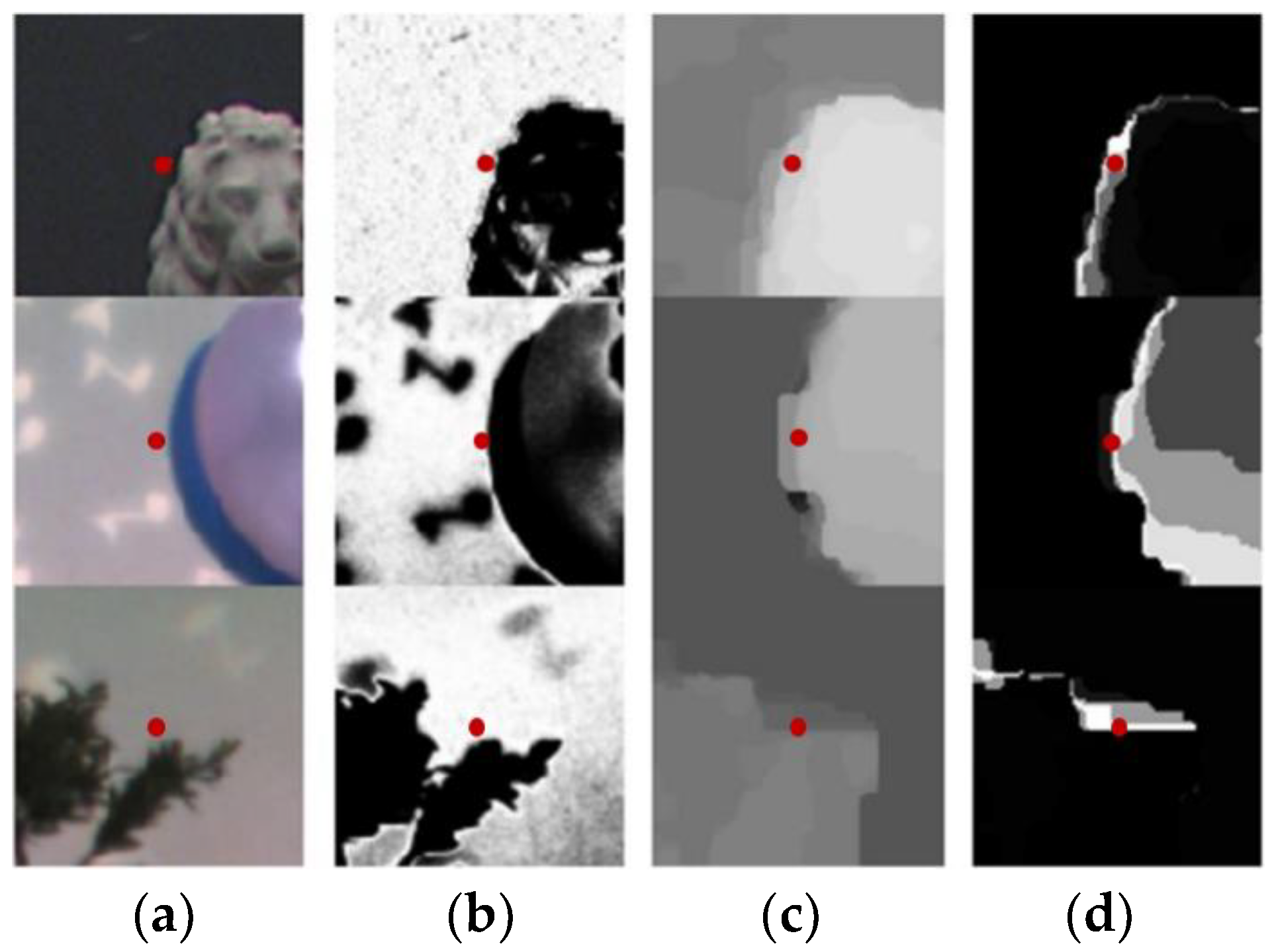
Figure 1 and Figure 2 illustrate the basic principle on how to measure the inconsistency of two collocated pixels in RGB and depth images with Equations (1) and (2). In Figure 1, the collocated pixels and are consistent in the three examples, both of which belong to the same object in RGB and depth images. We calculate and of the current pixel and the local window is set as the whole image patches. The white regions of the two weight maps well overlap with each other in these three examples. That means that most collocated pixels in the window have larger values in both the two weight maps of RGB and depth images. The larger the size of the window is, the more collocated pixels will have large values in both of the two weight maps. By comparison, the two collocated pixels at the location i in RGB and depth images are inconsistent in Figure 2, i.e., they do not belong to the same object in RGB and depth images. In these examples, the white regions of the two weight maps rarely overlap with each other. A few collocated pixels in the window have large values in both of the two weight maps.
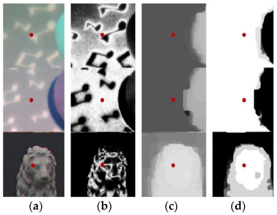
Figure 1.
Weight maps of RGB and depth images when two collocated pixels are consistent: (a) RGB image, (b) weight map of RGB, (c) depth image, and (d) weight map of depth image. The points in red denote two collocated pixels at the location i in RGB and depth images. White and black regions indicate pixels with large and small weight values, respectively.

Figure 2.
Weight maps of RGB and depth images when two collocated pixels are inconsistent: (a) RGB image, (b) weight map of RGB image, (c) depth image, and (d) weight map of depth image.
We then conclude the basic principle of the model as follows. When two collocated pixels and in RGB and depth images are consistent, a large number of collocated pixels nearby have large values in both of the two weight maps. On the contrary, when two collocated pixels and are inconsistent, a few collocated pixels have large values in both of the two weight maps. Then, the inconsistency of the collocated pixels in RGB image and in depth image can be determined by counting the number of pixels in the large-sized window . Larger pixel number indicates that the current pixel at the location i in depth image is inconsistent with its collocated one in RGB image; otherwise, they are consistent. A pixel near depth boundaries is considered to be an erroneous one when it is inconsistent with its collocated one in RGB image.
3.2. The RGB–Depth Boundary Inconsistency Model
3.2.1. Improving the Weights of RGB and Depth Images
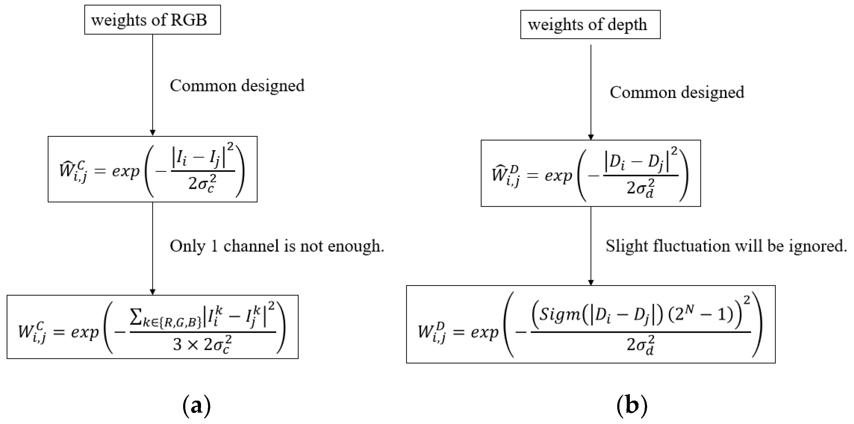
It has been concluded that Equations (1) and (2) could well represent the inconsistency of collocated pixels in RGB and depth images. The proposed model is derived from Equations (1) and (2). However, we further make a few changes by considering the characteristics of depth and RGB images. For the current pixel at the location i in RGB and depth images, we calculate the weight maps with Equations (3) and (4) instead in the large-sized window as follows:
Here, denotes the pixel at the location i in the k-th channel (i.e., R, G, and B) of RGB image, denotes the pixel at the location i in depth image, and N denotes the bit depth of depth image. We then elaborate the differences between the improved weights in Equations (3) and (4) and the ones in Equations (1) and (2).
Compared with Equation (1), Equation (3) jointly utilizes all three channels of RGB image. The reason lies in the fact that measuring the inconsistency of collocated pixels highly depends on the structures of objects in RGB image. However, a single channel may not fully represent the structures of the scene, e.g., a boundary in red may not be observed in the channels R and B of RGB image. In this scenario, the structures of the scene can be well measured by the improved weight in Equation (3).
Compared with Equation (2), Equation (4) replaces the similarity of depth image by the sigmod function , where
It is acknowledged that a depth image is generally composed of piece-wise smooth regions. So the weight is approximately to be either 0 or 1. However, due to the limitation of depth acquisition techniques, the values of depth pixels may fluctuate slightly inside the same object. In this scenario, the difference inside an object may be larger than 0 and the weight in Equation (2) may be much smaller than 1. The sigmod function in Equation (5) well alleviates this problem. Small difference can be mapped to nearly 0 by the sigmod function. The weight values is then set to nearly 1 with the improved weight in Equation (4) and vice versa. Therefore, the improved weight values of depth image is mainly composed of 0 and 1, which is in accordance with the piece-wise characteristics of depth image. We totally provide a structure diagram in Figure 3. It can be seen that our improved weights well hold the common problems of RGB-D weights.

Figure 3.
Diagram of the weights of RGB and depth images: (a) improvement of RGB weights; (b) improvement of depth weights.
3.2.2. Measuring the Inconsistency of Collocated Pixels
We then measure the inconsistency of two collocated pixels at the location i in depth and RGB images based on the weights in Equations (3) and (4). We have concluded most collocated pixels in the local window will have large values in both of the two weight maps when two collocated pixels are consistent. Otherwise, they are inconsistent. Our goal is to quantitatively measure the proportion of these collocated pixels inside the window based on the two weight maps and . We adopt the simple product operation for this purpose. Both and are within the range [0, 1]; thus, the produce values are also within the range [0, 1]. Large value of the product indicates that both the weight values and are large. On the contrary, small value of indicates that either or is small.
The inconsistency of the two collocated pixels at the location i in RGB and depth images is then quantitatively measured by accumulating the product values of all collocated pixels in the window as follows:
Larger value of indicates that a large number of pixels have large product values . Then, the two collocated pixels at the location i are expected to be more consistent with each other. Otherwise, smaller value of indicates that the two collocated pixels are more inconsistent. Note that the value of is related to the size of the local window . The larger the size of the window is, the more pixels may be involved. Consequently, the produce values of more pixels will be acculumated in Equation (6). Therefore, we further normalize the model in Equation (6) as follows:
The normalized value ranges within [0, 1]. In additional, it is independent of the size of the window.
Equation (7) provides the basic model to measure the inconsistency of two collocated pixels at the location i in depth and RGB images. It can be used in different applications. For example, we use this model to classify all pixels into erroneous ones and correct ones in depth image. To this end, we first binarize the model in Equation (7) as follows:
Here, denotes a predefined threshold T = 0.25 in our solution. In this way, all pixels in depth and RGB images are determined to be inconsistent () or consistent (). A pixel in depth image is determined to be erroneous when it is inconsistent with its collocated one in RGB image. This is because the pixel in RGB image is often correct. In this way, all erroneous pixels in depth image can be identified. Note that Equation (8) is not involved in the depth recovery method. It is only used as an example to identify erroneous pixels of depth images in the experiment.
4. Depth Image Rectification
It has been shown in Section 3.1 that erroneous boundaries are mainly induced by erroneous pixels and blurs in depth images. Our goal is to correct all erroneous pixels and remove the blurs near object boundaries with the guidance of reference RGB images. A lot of image processing frameworks can be adopted, such as the weighted mean filter (WMF) [21], bilateral filter [16], Gaussian filter, guided filter [19], weighted median filter [22], Markov random field [15], and graph model [18]. The developed model can be embedded into these frameworks for depth image rectification. In this paper, we adopt the simple but effective WMF [21], which suits for flat depth image with few textures. The ablation study of other filter methods will be shown in Section 5.4.
4.1. Framework of the General WMF
We first introduce the framework of the general WMF [21]. For a pixel at the location i in the input depth image, it is filtered by weighted-averaging all pixels in the local window centered at the location i as follows:
Here, and denote the values of pixels at the location i in input and output depth images, respectively. In the general WMF, the weight is often defined based on the values of pixels in the input depth image like the Gaussian weight in Equation (4). In order to recover the depth image with the guidance of a reference RGB image, the weight is generally designed based on the values of both depth and RGB images. For example, it can be achieved based on the bilateral filter as follows:
Here, and denote the Gaussian weights in Equations (3) and (4) based on RGB and depth images, respectively. In this way, the WMF preserves the object boundaries of the depth image with the guidance of the reference RGB image.
4.2. Weight Design Based on the Developed Model
In our method, we only update the weight of the WMF in Equation (9) based on the RGB–Depth boundary inconsistency model. It is known that the weight in Equation (10) often requires the structures of depth and RGB images to be well aligned. Unfortunately, depth images generally contain erroneous pixels near object boundaries of depth image. As a result, the structures of depth and RGB images are not well aligned near object boundaries. These erroneous pixels need to be corrected for depth image recovery. Therefore, these erroneous pixels of depth images need to be identified and inactivated in the WMF. The developed model can be adopted for this purpose. The model measures the inconsistency of collocated pixels in depth and RGB images and then identifies erroneous pixels in depth images based on Equation (7). We redesign the weight by considering erroneous pixels and correct ones in depth images separately.
For erroneous pixels in depth images, their values are incorrect and these pixels are inactivated in the weight of the WMF. In this case, we define the weight based on the weight of the RGB image as follows:
The weight denotes the inconsistency of the collocated pixels at the location j in depth and RGB images. In this way, the erroneous pixel at the location j in depth images is inactivated because the weight value is near to zero for erroneous pixels and near to 1 for correct ones.
For correct pixels in depth images, their values are correct and these pixels are used in the WMF. In this case, we define the weight based on the weight of depth images as follows:
Finally, the weight is defined by combining the two weights in Equations (11) and (12) as follows:
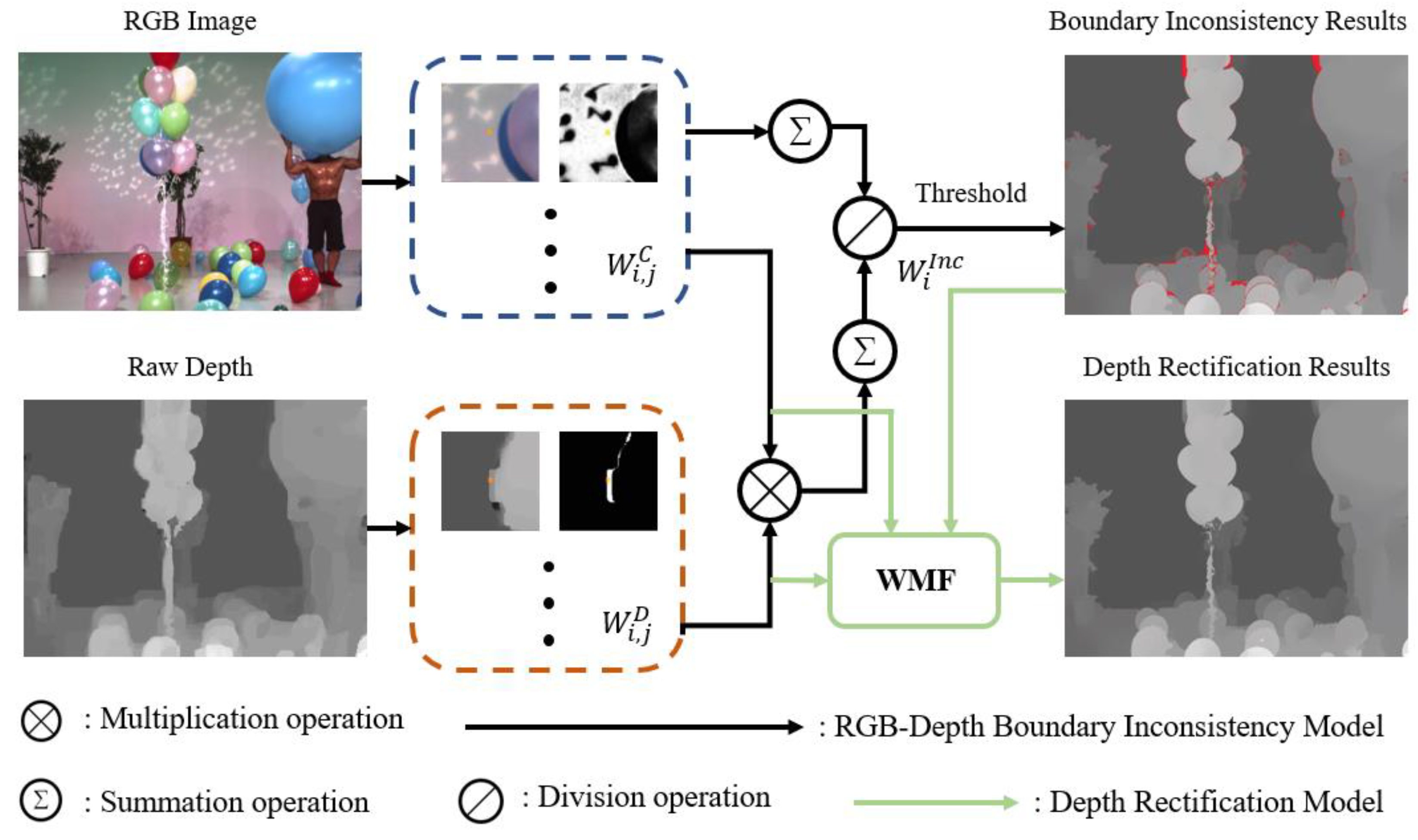
The depth image rectification method is realized by updating the weight of the WMF in Equation (9) with the one in Equation (13). With this method, erroneous pixels in depth images are corrected by correct pixels of RGB and depth images. Erroneous object boundaries of depth images are then rectified by correcting all identified erroneous pixels. Finally, the overall framework of our method is shown in Figure 4.

Figure 4.
The overall framework of our method.
5. Experiments and Analysis
5.1. Experiment Setting
Experiments were conducted on the dataset recommended by MPEG [44] and the Middlebury dataset [45]. Seven competitive baselines were used for comparison including the robust weighted least squares method (denoted “RWLS”) [37], the auto-regression based method (denoted “AR”) [36], the explicit edge inconsistency evaluation model (denoted “EEIE”) [41], and four recent learning-based methods, i.e., the dynamic guidance CNN (denoted “DGCNN”) [29], deformable kernel networks (denoted “DKN”) [30], the diffusion model for depth enhancement (denoted “DM”) [52], and structure-guided networks (denoted “SGN”) [53]. Note that the well-trained models of the DGCNN [29], DKN [30], DM [52], and SGN [53] released by the authors were directly adopted for fair comparison.
There are multiple parameters in the two improved weights in Equations (3) and (4). All these parameters are determined by training on our test dataset. First, our model requires the size of the local window to be large enough compared with erroneous regions in depth images. The radius of the window is finally fixed to be r = 30 for both of the two weights in Equations (3) and (4). Second, the standard variances in Equations (3) and (4) are set as to well differentiate the foreground from the background in RGB and depth images. Third, the two parameters of the sigmod function in Equation (5) are set as . In addition, N in Equation (4) is generally set as 8 for 8-bit depth images.
5.2. Visual Results
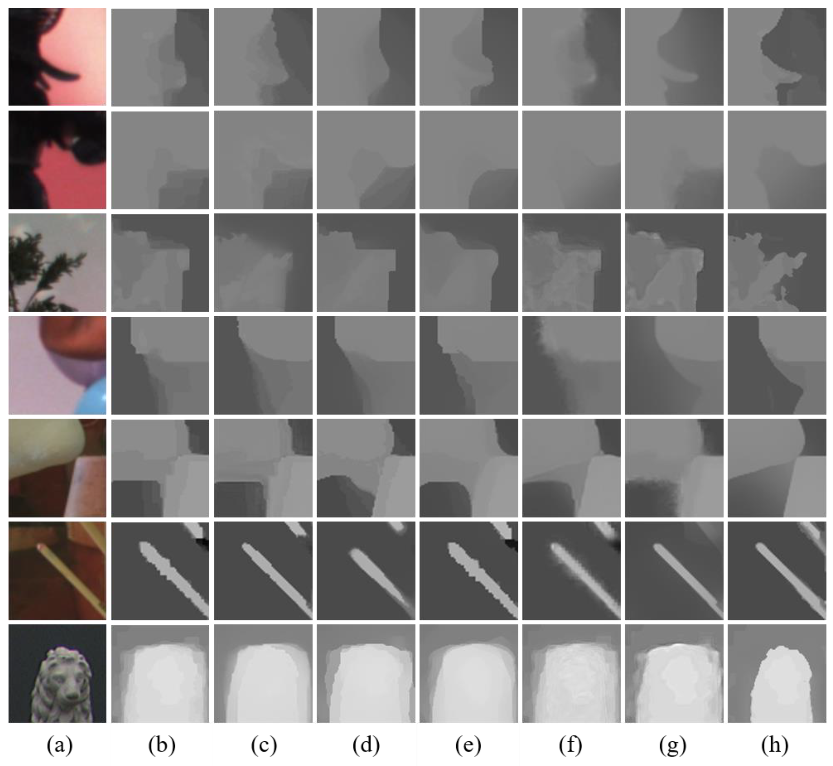
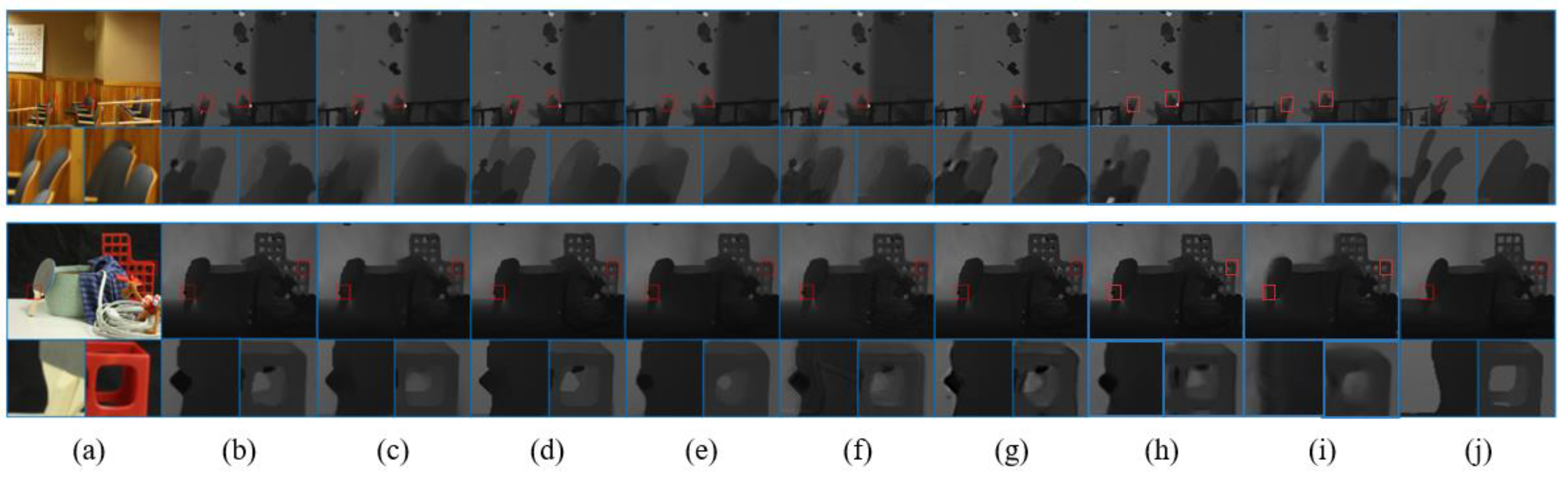
We first show the visual results of the depth image rectification method. Figure 5 show some enlarged depth images, which are from the whole depth images in Figure 6 and Figure 7. It is clear that object boundaries in raw depth images are distorted seriously by erroneous pixels. Figure 5h shows that the proposed method fully removes erroneous pixels near object boundaries in depth images. Thereby, erroneous object boundaries are rectified accurately. The results in the first, third, and sixth rows of Figure 5 show that the proposed method even well rectifies tiny object boundaries in depth images. The object boundaries in all these rectified depth images in Figure 5h are very clear and sharp. By comparison, most the baseline methods well smooth flat regions in depth images. However, they fail to rectify erroneous object boundaries in depth images as in Figure 5c–g. In these results, a large number of erroneous pixels still remained in recovered depth images. For example, the method AR in Figure 5c well smoothed the flat regions. However, this method did not fully correct erroneous pixels and remove blurs near depth boundaries. Similarly, the RWLS method in Figure 5d and EIEF method in Figure 5e well remove blurs near depth boundaries. However, erroneous pixels are not well corrected. The results of the two learning-based methods, the DGCNN and DKN, in Figure 5f and Figure 5g are similar. Figure 6 and Figure 7 further show the results on whole depth images. It is seen that most erroneous object boundaries in depth images are rectified accurately compared with the baseline methods.

Figure 5.
Enlarged examples of rectified depth images: (a) RGB image, (b) raw depth, (c) AR [36], (d) RWLS [37], (e) EIEF [41], (f) DGCNN [29], (g) DKN [30], and (h) proposed.
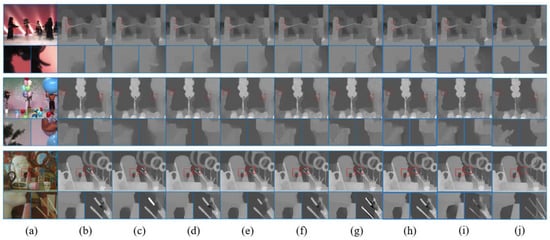
Figure 6.
Visual results of on whole depth images from the MPEG dataset: (a) RGB image, (b) raw depth, (c) AR [36], (d) RWLS [37], (e) EIEF [41], (f) DGCNN [29], (g) DKN [30], (h) DM [52], (i) SGN [53], and (j) proposed.
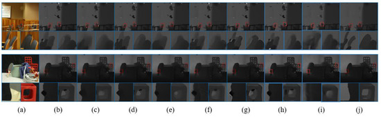
Figure 7.
Visual results on whole depth images from the Middlebury2014 dataset: (a) RGB image, (b) raw depth, (c) AR [36], (d) RWLS [37], (e) EIEF [41], (f) DGCNN [29], (g) DKN [30], (h) DM [52], (i) SGN [53], and (j) proposed.
The effectiveness of a depth image rectification method benefits from the RGB–Depth boundary inconsistency model. In our solution, erroneous pixels in depth images are identified explicitly by the developed model. Erroneous object boundaries in depth images are accurately rectified by correcting these erroneous pixels. By comparison, most baseline methods do not explicitly identify and correct erroneous pixels in depth images. As a result, erroneous object boundaries in depth images cannot be rectified accurately such as in the results in Figure 5, Figure 6 and Figure 7.
5.3. Quantitative Results
We then test the quantitative results of the depth image rectification method. Table 1 concludes the RMSE values on Middlebury2014. The proposed method considerably improves the RMSE of recovered depth images by 1.56~3.34 (2.91 on average) compared with the seven baseline methods. Indeed, the proposed method outperforms the baseline methods on most individual examples as in Table 1. The effectiveness of the proposed method benefits from the RGB–Depth boundary inconsistency model. The baseline methods could well smooth flat regions of depth images; however, erroneous object boundaries could not be well rectified. By comparison, the developed model identifies most erroneous pixels in depth images. These erroneous pixels are fully corrected by the depth image rectification method. Table 2 concludes the SSIM results on Middlebury2014. The proposed method improves the SSIM values of recovered depth images by 0.011~0.060 (0.029 on average). Similar to what is shown in Table 1, the proposed method outperforms the baseline methods on most individual test examples.

Table 1.
RMSE values for Middlesbury2014 (lower is better). The best results are in bold.
Table 2.
SSIM values for Middlesbury2014 (larger is better).
Notably, the recent learning-based methods [29,30,52,53] do not work well, as shown in Table 1. The reason lies in two aspects. On the one hand, learning-based methods generally require large-scale datasets with both GT and low-quality depth images for training. Unfortunately, most public datasets do not contain low-quality depth images. On the other hand, GT depth images in these public datasets still include a few erroneous object boundaries due to the limitations of depth acquisition techniques. As a result, misalignment occurs between GT depth images and reference RGB images. However, most learning-based methods are trained on well-aligned datasets. Some recent learning-based methods such as DM [52] and SGN methods [53] may perform better than the DGCNN [29] and DKN [30] methods. But they still suffer from the misalignment of RGB and GT depth images.
5.4. Ablation Study
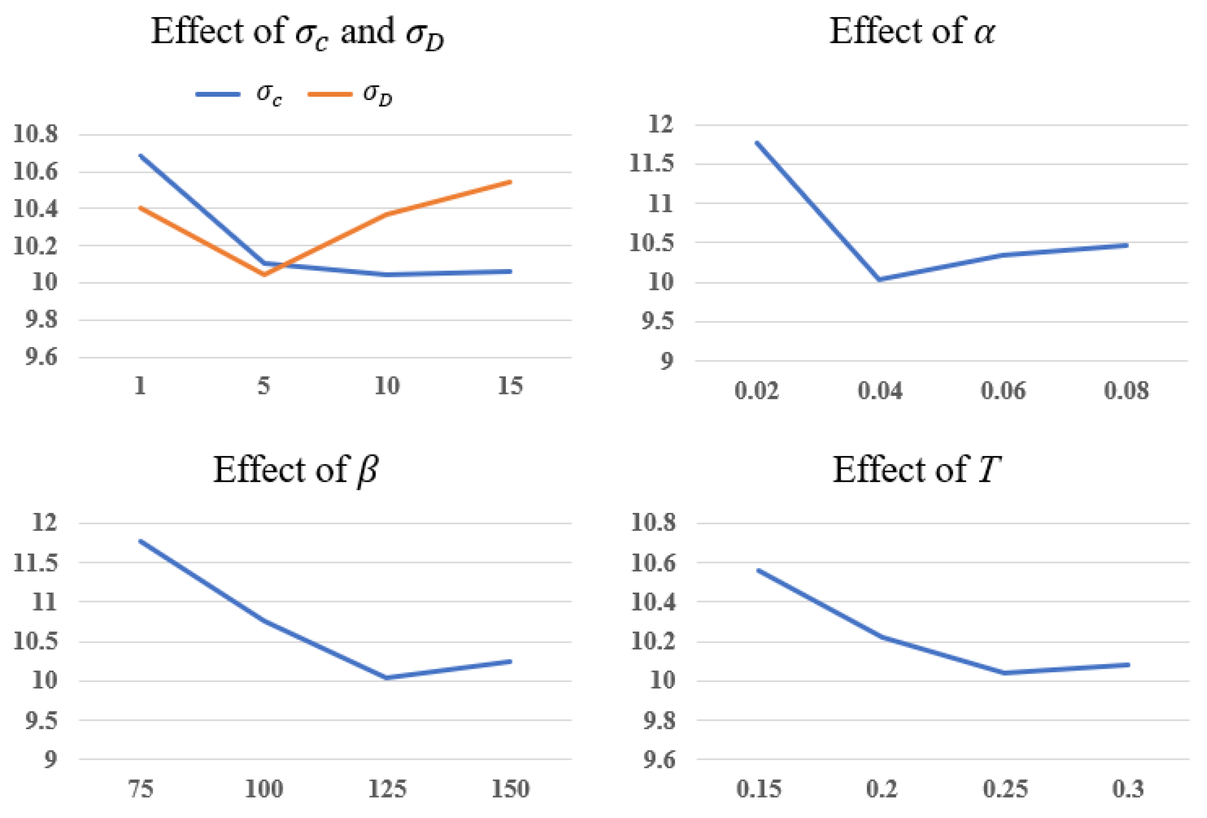
Parameter analysis: Figure 8 gives the analysis of parameters in our model, including in Equation (3), in Equation (4), α and β in Equation (5), and T in Equation (8). We adopt the metric RMSE in Middlebury2014 to analyze the parameters. First, and are increased from 1 to 15 at the interval of 5. These two parameters control the variance of the Gaussian function. We verify that the best choice for is 10 and the best choice for is 5. The results also demonstrate that our model performs best when α equals 0.04, β equals 125, and T equals 0.25.
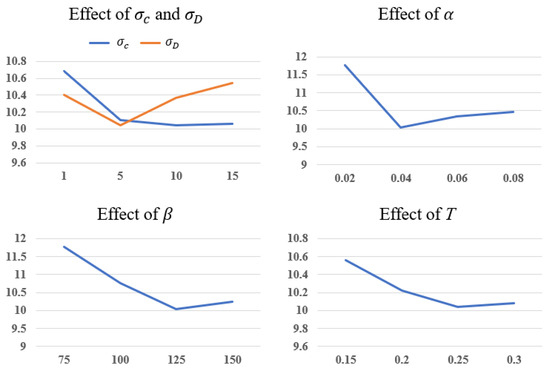
Figure 8.
Analysis of parameters in our model.
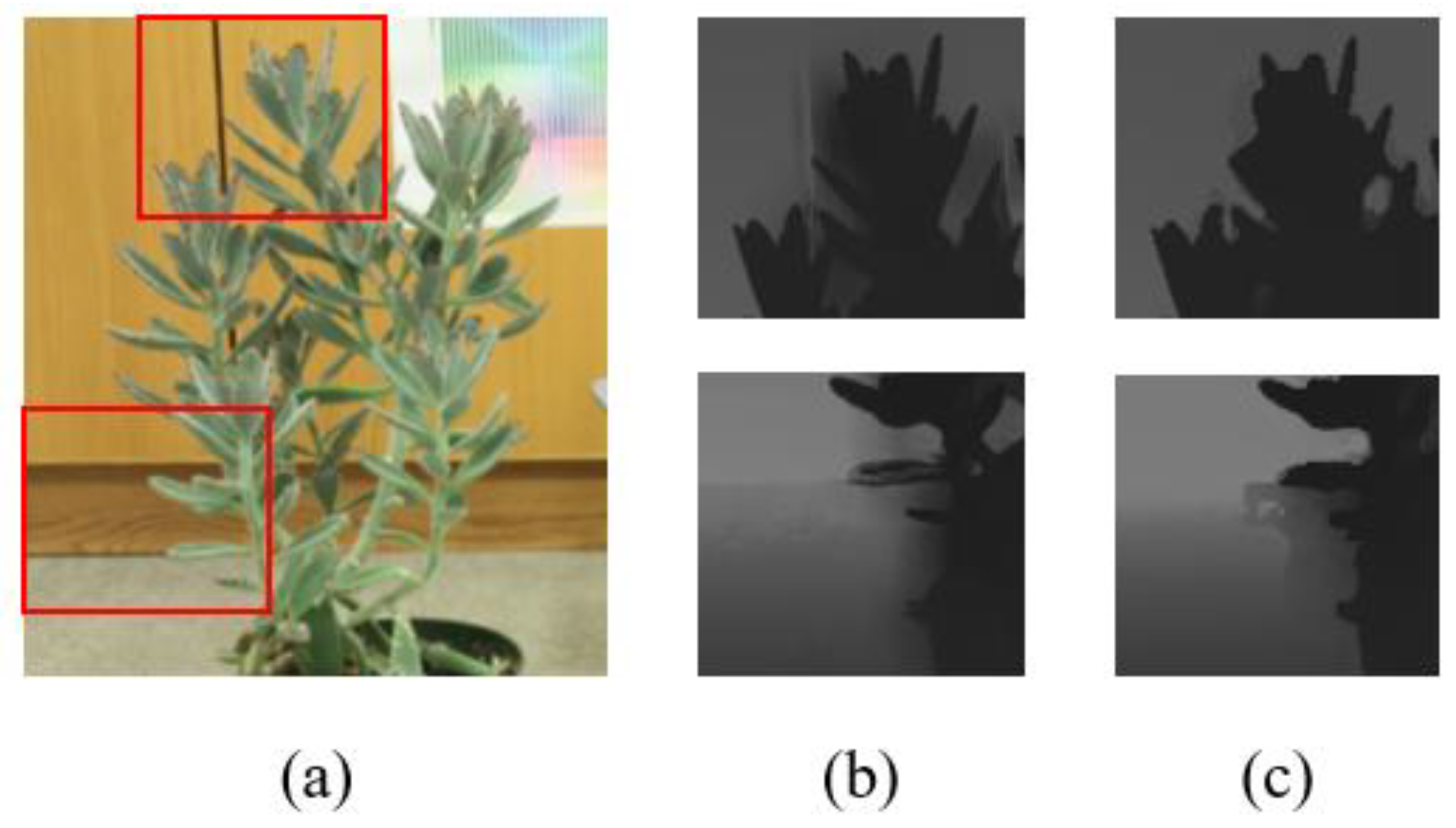
Ablation study for RGB–Depth boundary inconsistency model: For pair comparison, we also provide the results of the WMF method without our RGB–Depth boundary inconsistency model (denoted “BIM”). While removing the BIM, the framework will be degraded as a common WMF [21], denoted as ”w/o BIM”. Our final model is denoted “with BIM”. The quantitative results in Table 3 demonstrate the effectiveness of our RGB–Depth boundary inconsistency model. It can be seen that the BIM works better than ‘without BIM’ using the RMSE but 0.002 worse using the SSIM. This is because the WMF equipped with our boundary inconsistency model works better near depth edges. However, some unnecessary sharp edges in depth maps lead to the degradation of the SSIM. This phenomenon is also verified by the qualitative results in Figure 9.
Table 3.
Ablation study of RGB–Depth boundary inconsistency model.

Figure 9.
Ablation study of boundary inconsistency model: (a) RGB, (b), w/o BIM, and (c) with BIM.
Ablation study of different filter methods: As explained in Section 4, our RGB–Depth boundary inconsistency model can be applied to other filter methods. In Table 4, we replace the WMF with two other filters including the weighted median filter [22] (denoted as “median”) and guided filter [19] (denoted as “guided”). Our final solution based on weighted mean filter is denoted as “mean”. The results demonstrate that our final solution based on the WMF achieves the best performance.
Table 4.
Ablation study of different filter methods.
6. Conclusions and Discussion
In this paper, a simple yet effective RGB–Depth boundary inconsistency model has been developed to identify erroneous pixels in raw depth images. A depth image rectification method has then been proposed by embedding the model into a weighted mean filter (WMF) to rectify erroneous object boundaries in depth images. Experiment results have verified that the proposed method outperforms recent optimization-based methods and learning-based methods. Our future work will focus on two aspects. On the one hand, the robustness of the method needs to be well improved. On the other hand, the developed model can be combined with learning-based methods to improve the accuracy.
Author Contributions
Conceptualization, X.Z. and M.Y.; methodology, H.C., X.Z. and M.Y.; software, H.C. and M.Y.; validation, H.C., X.Z., A.L. and M.Y.; formal analysis, H.C., X.Z. and M.Y.; investigation, X.Z. and M.Y.; resources, X.Z. and M.Y.; data curation, H.C. and M.Y.; writing—original draft preparation, H.C. and M.Y.; writing—review and editing, H.C., X.Z., A.L. and M.Y.; visualization, H.C. and M.Y.; supervision, M.Y.; project administration, X.Z. and M.Y.; funding acquisition, X.Z. and M.Y. All authors have read and agreed to the published version of the manuscript.
Funding
This research was funded by the Scientific Research Project of the Shaanxi Provincial Department of Transportation, grant number 24-81K, and Scientific and Technological Innovation Projects of Shaanxi Provincial State-owned Capital Operation Budget Special Fund, grant number 2023-017.
Data Availability Statement
Derived data supporting the findings of this study are available from the corresponding author on request.
Conflicts of Interest
Authors H.C. and X.Z. were employed by the company Shaanxi Provincial Transport Planning Design and Research Institute. The remaining authors declare that the research was conducted in the absence of any commercial or financial relationships that could be construed as a potential conflict of interest.
References
- Sun, J.; Zheng, N.; Shum, H. Stereo matching using belief propagation. IEEE Trans. Pattern. Anal. Mach. Intell. 2003, 25, 787–800. [Google Scholar]
- Saxena, A.; Sun, M.; Ng, A.Y. Make3D: Learning 3D scene structure from a single still image. IEEE Trans. Pattern Anal. Mach. Intell. 2009, 31, 824–840. [Google Scholar] [CrossRef] [PubMed]
- Fu, H.; Gong, M.; Wang, C.; Batmanghelich, K.; Tao, D. Deep ordinal regression network for monocular depth estimation. In Proceedings of the IEEE Conference on Computer Vision and Pattern Recognition, Salt Lake City, UT, USA, 18–23 June 2018; pp. 2002–2011. [Google Scholar]
- Lee, J.; Heo, M.; Kim, K.; Kim, C. Single-image depth estimation based on Fourier domain analysis. In Proceedings of the IEEE Conference on Computer Vision and Pattern Recognition, Salt Lake City, UT, USA, 18–23 June 2018; pp. 330–339. [Google Scholar]
- Zanuttigh, P.; Marin, G.; Dal Mutto, C.; Dominio, F.; Minto, L.; Cortelazzo, G.M. Time-of-Flight and Stucture Light Depth Cameras; Springer: Cham, Switzerland, 2016. [Google Scholar]
- Qiao, Y.; Jiao, L.; Yang, S.; Hou, B.; Feng, J. Color correction and depth-based hierarchical hole filling in free viewpoint generation. IEEE Trans. Broadcast. 2019, 65, 294–307. [Google Scholar] [CrossRef]
- Li, F.; Li, Q.; Zhang, T.; Niu, Y.; Shi, G. Depth acquisition with the combination of structured light and deep learning stereo matching. Signal Process. Image Commun. 2019, 75, 111–117. [Google Scholar] [CrossRef]
- Chen, Z.; Zhou, W.; Li, W. Blind stereoscopic video quality assessment: From depth perception to overall experience. IEEE Trans. Image Process. 2017, 27, 721–734. [Google Scholar] [CrossRef] [PubMed]
- Liao, T.; Li, N. Natural language stitching using depth maps. arXiv 2022, arXiv:2202.06276. [Google Scholar]
- Criminisi, A.; Perez, P.; Toyama, K. Region Filling and Object Removal by Exemplar-Based Image Inpainting. IEEE Trans. Image Process. 2004, 13, 1200–1212. [Google Scholar] [CrossRef]
- Xue, H.; Zhang, S.; Cai, D. Depth image inpainting: Improving low rank matrix completion with low gradient regularization. IEEE Trans. Image Process. 2017, 26, 4311–4320. [Google Scholar] [CrossRef]
- Part, S.C.; Kyu, M.K.; Kang, M.G. Super-resolution image reconstruction: A technical overview. IEEE Signal Process. Mag. 2003, 20, 21–26. [Google Scholar]
- Xie, J.; Feris, R.S.; Yu, S.-S.; Sun, M.-T. Joint super resolution and denoising from a single depth image. IEEE Trans. Multimed. 2015, 17, 1525–1537. [Google Scholar] [CrossRef]
- Xie, J.; Feris, R.S.; Sun, M.-T. Edge-guided single depth image super resolution. IEEE Trans. Image Process. 2016, 25, 428–438. [Google Scholar] [CrossRef] [PubMed]
- Min, D.; Choi, S.; Lu, J.; Ham, B.; Sohn, K.; Do, M.N. Fast global image smoothing based on weighted least squares. IEEE Trans. Image Process. 2014, 23, 5638–5653. [Google Scholar] [CrossRef] [PubMed]
- Tomasi, C.; Manduchi, R. Bilateral filtering for gray and color images. In Proceedings of the IEEE International Conference on Computer Vision, Bombay, India, 4–7 January 1998; pp. 839–846. [Google Scholar]
- Yang, J.; Ye, X.; Frossard, P. Global auto-regressive depth recovery via iterative non-local filtering. IEEE Trans. Broadcast. 2019, 65, 123–137. [Google Scholar] [CrossRef]
- Liu, X.; Zhai, D.; Chen, R.; Ji, X.; Zhao, D.; Gao, W. Depth super-resolution via joint color-guided internal and external regularizations. IEEE Trans. Image Process. 2019, 28, 1636–1645. [Google Scholar] [CrossRef]
- He, K.; Sun, J.; Tang, X. Guided image filtering. IEEE Trans. Pattern Anal. Mach. Intell. 2013, 35, 1397–1409. [Google Scholar] [CrossRef]
- Yang, Y.; Lee, H.S.; Oh, B.T. Depth map upsampling with a confidence-based joint guided filter. Signal Process. Image Commun. 2019, 77, 40–48. [Google Scholar] [CrossRef]
- Zhang, P.; Li, F. A new adaptive weighted mean filter for removing salt-and-pepper noise. IEEE Signal Process. Lett. 2014, 21, 1280–1283. [Google Scholar] [CrossRef]
- Ma, Z.; He, K.; Wei, Y.; Sun, J.; Wu, E. Constant time weighted median filtering for stereo matching and beyond. In Proceedings of the IEEE International Conference on Computer Vision, Columbus, OH, USA, 23–28 June 2014; pp. 49–56. [Google Scholar]
- Zhang, H.; Zhang, Y.; Wang, H.; Ho, Y.S.; Feng, S. WLDISR: Weighted local sparse representation-based depth image super-resolution for 3D video system. IEEE Trans. Image Process. 2019, 28, 561–576. [Google Scholar] [CrossRef]
- Chen, B.; Jung, C. Single depth image super-resolution using convolutional neural networks. In Proceedings of the 2018 IEEE International Conference on Acoustics, Speech and Signal Processing, Calgary, AB, Canada, 15–20 April 2018; pp. 1473–1477. [Google Scholar]
- Ye, X.; Duan, X.; Li, H. Depth super-resolution with deep edge-inference network and edge-guided depth filling. In Proceedings of the 2018 IEEE International Conference on Acoustics, Speech and Signal Processing, Calgary, AB, Canada, 15–20 April 2018; pp. 1398–1402. [Google Scholar]
- Wen, Y.; Sheng, B.; Li, P.; Lin, W.; Feng, D.D. Deep color guided coarse-to-fine convolutional network cascade for depth image super-resolution. IEEE Trans. Image Process. 2019, 28, 994–1006. [Google Scholar] [CrossRef]
- Ni, M.; Lei, J.; Cong, R.; Zheng, K.; Peng, B.; Fan, X. Color-guided depth map super resolution using convolutional neural network. IEEE Access 2017, 5, 26666–26672. [Google Scholar] [CrossRef]
- Jiang, Z.; Yue, H.; Lai, Y.-K.; Yang, J.; Hou, Y.; Hou, C. Deep edge map guided depth super resolution. Signal Process. Image Commun. 2021, 90, 116040. [Google Scholar] [CrossRef]
- Gu, S.; Guo, S.; Zuo, W.; Chen, Y.; Timofte, R.; Van Gool, L.; Zhang, L. Learned dynamic guidance for depth image reconstruction. IEEE Trans. Pattern Anal. Mach. Intell. 2020, 42, 2437–2452. [Google Scholar] [CrossRef]
- Kim, B.; Ponce, J.; Ham, B. Deformable kernel networks for joint image filtering. Int. J. Comput. Vis. 2020, 129, 579–600. [Google Scholar] [CrossRef]
- Zhu, C.; Zhao, Y.; Yu, L. 3D-TV System with Depth-Image-Based Rendering: Architectures, Techniques and Challenges; Springer: New York, NY, USA, 2013. [Google Scholar]
- Zhao, Y.; Zhu, C.; Chen, Z.; Yu, L. Depth no-synthesis-error model for view synthesis in 3-D video. IEEE Trans. Image Process. 2011, 20, 2221–2228. [Google Scholar] [CrossRef] [PubMed]
- Zhu, C.; Li, S.; Zheng, J.; Gao, Y.; Yu, L. Texture-aware depth prediction in 3D video coding. IEEE Trans. Broadcast. 2016, 62, 482–486. [Google Scholar] [CrossRef]
- Yuan, H.; Kwong, S.; Wang, X.; Zhang, Y.; Li, F. A virtual view PSNR estimation method for 3-D videos. IEEE Trans. Broadcast. 2016, 62, 134–140. [Google Scholar] [CrossRef]
- Xu, X.; Po, L.-M.; Ng, K.-H.; Feng, L.; Cheung, K.-W.; Cheung, C.-H.; Ting, C.-W. Depth map misalignment correction and dilation for DIBR view synthesis. Signal Process. Image Commun. 2013, 28, 1023–1045. [Google Scholar] [CrossRef]
- Yang, J.; Ye, X.; Li, K.; Hou, C.; Wang, Y. Color-guided depth recovery from RGB-D data using an adaptive autoregressive model. IEEE Trans. Image Process. 2014, 23, 3443–3458. [Google Scholar] [CrossRef]
- Liu, W.; Chen, X.; Yang, J.; Wu, Q. Robust color guided depth map restoration. IEEE Trans. Image Process. 2017, 26, 315–327. [Google Scholar] [CrossRef]
- Jiang, Z.; Hou, Y.; Yue, H.; Yang, J.; Hou, C. Depth super-resolution from RGB-D pairs with transform and spatial domain regularization. IEEE Trans. Image Process. 2018, 27, 2587–2602. [Google Scholar] [CrossRef]
- Liu, X.; Zhai, D.; Chen, R.; Ji, X.; Zhao, D.; Gao, W. Depth restoration from RGB-D data via joint adaptive regularization and thresholding on manifolds. IEEE Trans. Image Process. 2019, 28, 1068–1079. [Google Scholar] [CrossRef]
- Dong, W.; Shi, G.; Li, X.; Peng, K.; Wu, J.; Guo, Z. Color-guided depth recovery via joint local structural and nonlocal low-rank regularization. IEEE Trans. Multimedia 2017, 19, 293–301. [Google Scholar] [CrossRef]
- Zuo, Y.; Wu, Q.; Zhang, J.; An, P. Explicit edge inconsistency evaluation model for color-guided depth map enhancement. IEEE Trans. Circuits Syst. Video Technol. 2018, 28, 439–453. [Google Scholar] [CrossRef]
- Xiang, S.; Yu, L.; Chen, C.W. No-reference depth assessment based on edge misalignment errors for t + d images. IEEE Trans. Image Process. 2016, 25, 1479–1494. [Google Scholar] [CrossRef]
- Jiao, J.; Wang, R.; Wang, W.; Li, D.; Gao, W. Color image-guided boundary-inconsistent region refinement for stereo matching. IEEE Trans. Circuits Syst. Video Technol. 2017, 27, 1155–1159. [Google Scholar] [CrossRef]
- Domanski, M.; Grajek, T.; Klimaszewski, K.; Kurc, M.; Stankiewicz, O.; Stankowski, J.; Wegner, K. Multiview Video Test Sequences and Camera Parameters, Document M17050, ISO/IEC JTC1/SC29/WG11 MPEG, Oct. 2009. Available online: https://www.mpeg.org/ (accessed on 19 August 2024).
- Scharstein, D.; Pal, C. Learning conditional random fields for stereo. In Proceedings of the IEEE/CVF Conference on Computer Vision and Pattern Recognition, Minneapolis, MN, USA, 14–19 June 2007; pp. 1–8. [Google Scholar]
- Liu, W.; Chen, X.; Yang, J.; Wu, Q. Variable bandwidth weighting for texture copy artifacts suppression in guided depth upsampling. IEEE Trans. Circuits Syst. Video Technol. 2017, 27, 2072–2085. [Google Scholar] [CrossRef]
- Lei, J.; Li, L.; Yue, H.; Wu, F.; Ling, N.; Hou, C. Depth map super-resolution considering view synthesis quality. IEEE Trans. Image Process. 2017, 26, 1732–1745. [Google Scholar] [CrossRef]
- Wang, Y.; Zhang, J.; Liu, Z.; Wu, Q.; Zhang, Z.; Jia, Y. Depth super-resolution on RGB-D video sequences with large displacement 3D motion. IEEE Trans. Image Process. 2018, 27, 3571–3585. [Google Scholar] [CrossRef]
- Jung, S.-W. Enhancement of image and depth map using adaptive joint trilateral filter. IEEE Trans. Circuits Syst. Video Technol. 2013, 23, 258–269. [Google Scholar] [CrossRef]
- Lo, K.-H.; Wang, Y.-C.F.; Hua, K.-L. Edge-preserving depth map upsampling by joint trilateral filter. IEEE Trans. Cybern. 2018, 48, 371–384. [Google Scholar] [CrossRef]
- Yang, Q.; Ahuja, N.; Yang, R.; Tan, K.-H.; Davis, J.; Culbertson, B.; Apostolopoulos, J.; Wang, G. Fusion of median and bilateral filtering for range image upsampling. IEEE Trans. Image Process. 2013, 22, 4841–4852. [Google Scholar] [CrossRef] [PubMed]
- Metzger, N.; Daudt, R.-C.; Schindler, K. Guided depth super-resolution by deep anisotropic diffusion. In Proceedings of the IEEE/CVF Conference on Computer Vision and Pattern Recognition, Vancouver, BC, Canada, 17–24 June 2023; pp. 18237–18246. [Google Scholar]
- Wang, Z.; Yan, Z.; Yang, J. SGNet: Structure guided network via gradient-frequency awareness for depth map super-resolution. In Proceedings of the 38th Annual AAAI Conference on Artificial Intelligence, Vancouver, BC, Canada, 20–27 February 2024; pp. 5823–5831. [Google Scholar]


Disclaimer/Publisher’s Note: The statements, opinions and data contained in all publications are solely those of the individual author(s) and contributor(s) and not of MDPI and/or the editor(s). MDPI and/or the editor(s) disclaim responsibility for any injury to people or property resulting from any ideas, methods, instructions or products referred to in the content. |
© 2024 by the authors. Licensee MDPI, Basel, Switzerland. This article is an open access article distributed under the terms and conditions of the Creative Commons Attribution (CC BY) license (https://creativecommons.org/licenses/by/4.0/).