
Real-Time Dense Visual SLAM with Neural Factor Representation


Abstract
1. Introduction
- We propose a novel scene representation based on neural factors, demonstrating higher-quality scene reconstruction and a more compact model memory footprint in large-scale scenes.
- In order to address insufficient real-time performance due to high MLP query costs in previous neural implicit SLAM methods, we introduce an efficient rendering approach using feature integration. This improves real-time performance without relying on a customized CUDA framework.
- We conducted extensive experiments on both synthetic and real-world datasets to validate our design choices, achieving competitive performance against baselines in terms of 3D reconstruction, camera localization, runtime, and memory usage.
2. Related Work
2.1. Traditional Dense Visual SLAM
2.2. Neural Implicit Representations
2.3. Neural Implicit Dense Visual SLAM
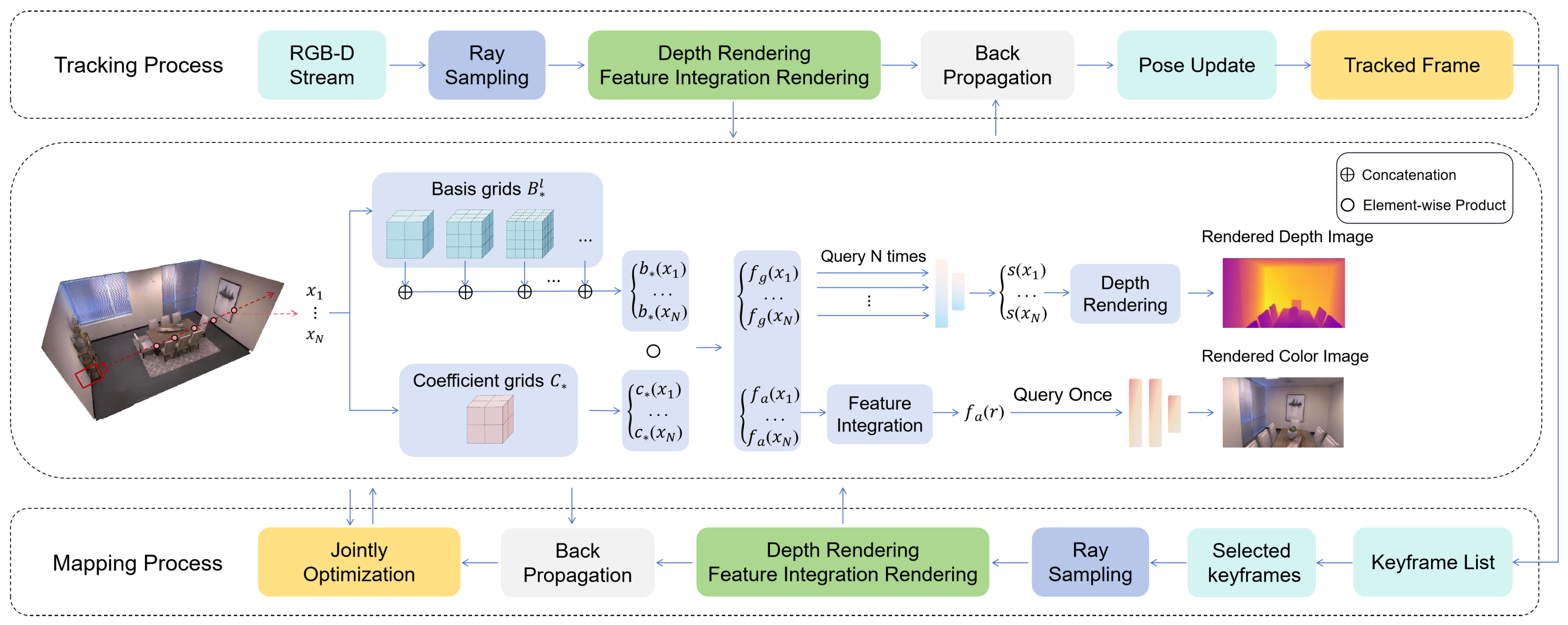
3. Method
3.1. Neural Factors Representation
3.2. Feature Integration Rendering
3.3. Training
3.3.1. Loss Functions
3.3.2. Tracking
3.3.3. Mapping
4. Experiments
4.1. Experimental Setup
4.1.1. Datasets
4.1.2. Baselines
4.1.3. Evaluation Metrics
4.1.4. Hyperparameters
4.1.5. Post-Processing
4.2. Reconstruction Evaluation
4.3. Camera Localization Evaluation
4.4. Runtime and Memory Usage Analysis
4.5. Ablation Study
5. Conclusions
- (1)
- We propose a novel scene representation method for neural implicit SLAM that encodes both the geometric and appearance information of a scene as a combination of the basis and coefficient factors. Compared to existing state-of-the-art methods, this representation not only enables higher-quality scene reconstruction but also exhibits a more stable memory growth rate when dealing with incremental reconstruction tasks for large-scale scenes. Furthermore, by employing multi-level tensor grids for the basis factors and a single-level tensor grid for the coefficient factors, our method can more accurately model high-frequency detail regions within the scene. Additionally, this representation significantly enhances camera localization accuracy, thereby demonstrating greater robustness in large-scale scenes.
- (2)
- In order to enhance the rendering efficiency of neural implicit SLAM, we introduce an efficient rendering approach based on feature integration. Feature integration rendering calculates the approximate features of rays by using a weighted summation of the features at sampling points and then feeds these into a shallow MLP to decode the final pixel colors. Compared to traditional volumetric rendering methods, this rendering approach significantly reduces the number of MLP queries during the color rendering stage, thereby improving real-time performance. Additionally, our method does not rely on customized CUDA frameworks, offering better scalability.
- (3)
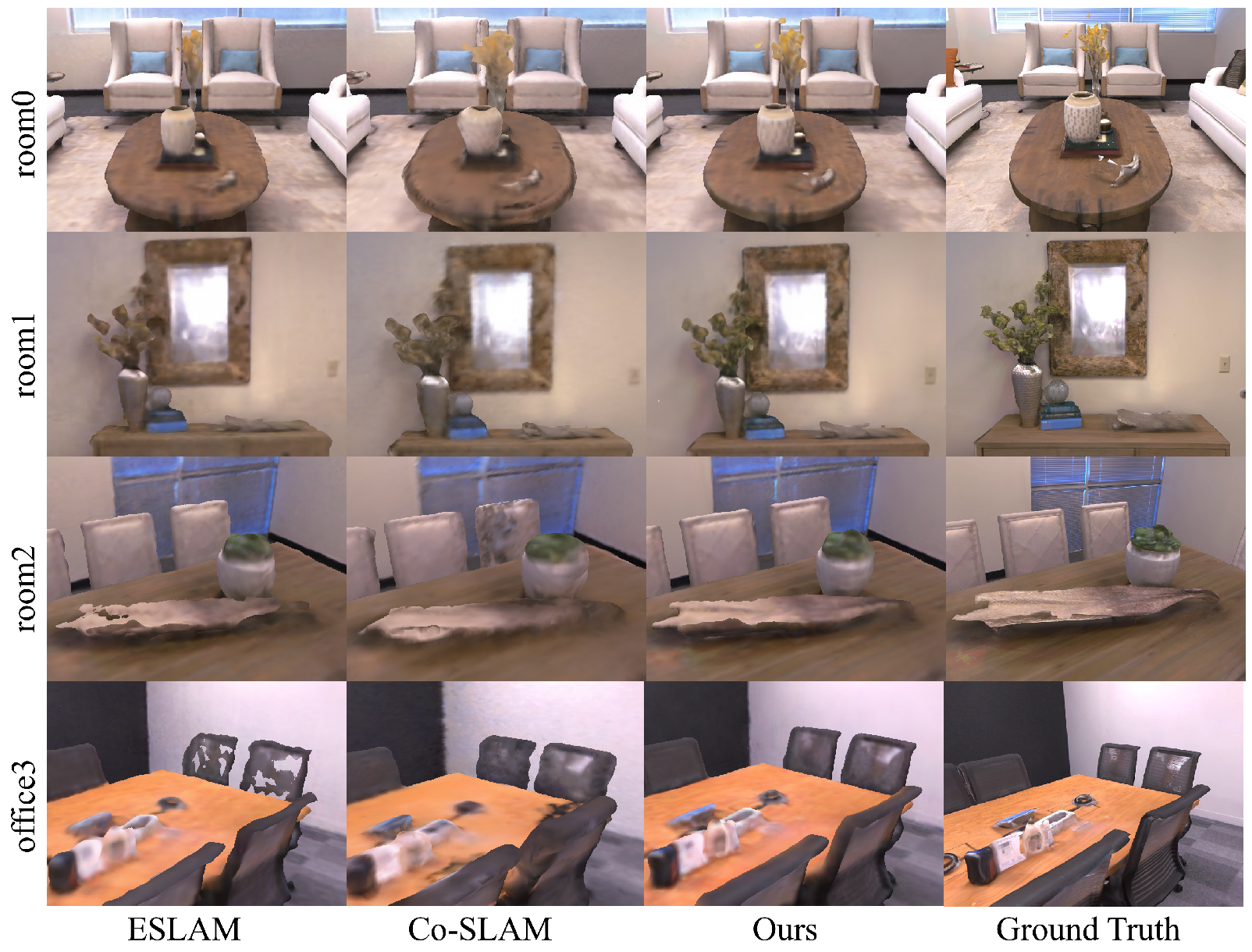
- We conducted extensive experiments on both synthetic and real-world datasets to validate our design choices. Our method shows competitive performance compared to existing state-of-the-art methods in terms of 3D reconstruction, camera localization, runtime, and memory usage. Specifically, for 3D reconstruction, we demonstrate both qualitative and quantitative results for the Replica dataset [28] and qualitative results for the ScanNet dataset [29]. The qualitative results indicate that our method performs better in regions with complex details. In terms of quantitative results, our method’s Depth L1 average outperforms other methods by 61%. For camera localization, we conduct comprehensive quantitative evaluations across three datasets, and our method’s ATE RMSE average improves by 75%, 46%, and 68%, respectively, compared to existing state-of-the-art methods. We validate the effectiveness of feature integration rendering through a series of ablation studies. In terms of color rendering, our method achieves a 60% speedup compared to traditional volume rendering while maintaining nearly the same PSNR. Additionally, we conduct quantitative experiments to analyze the memory footprint of our method. As the scene map grows, the memory usage of our method remains stable. Even though ESLAM [7] employs feature compression, our method remains competitive in large-scale scenes.
- (1)
- Our approach does not use compression storage for factor grids, which maintains high memory efficiency for large-scale scenes but still consumes memory resources for small-scale or object-centric scenes. Future work will explore more memory-efficient scene representation methods to enhance memory usage efficiency without compromising localization accuracy and reconstruction quality.
- (2)
- Due to the utilization of feature integration rendering, our method is prone to artifacts in color rendering when dealing with input frames that have extreme motion blur. In order to address this challenge, future work will focus on designing a deblurring process for the neural implicit SLAM framework. This process will perform blur detection and processing operations on each input frame, ensuring consistency of scene content across multi-view inputs. Consequently, this will enhance the robustness of our neural implicit SLAM method in the presence of extreme motion blur situations.
Author Contributions
Funding
Data Availability Statement
Acknowledgments
Conflicts of Interest
References
- Mur-Artal, R.; Montiel, J.M.M.; Tardos, J.D. ORB-SLAM: A versatile and accurate monocular SLAM system. IEEE Trans. Robot. 2015, 31, 1147–1163. [Google Scholar] [CrossRef]
- Mur-Artal, R.; Tardós, J.D. Orb-slam2: An open-source slam system for monocular, stereo, and rgb-d cameras. IEEE Trans. Robot. 2017, 33, 1255–1262. [Google Scholar] [CrossRef]
- Campos, C.; Elvira, R.; Rodríguez, J.J.G.; Montiel, J.M.; Tardós, J.D. Orb-slam3: An accurate open-source library for visual, visual–inertial, and multimap slam. IEEE Trans. Robot. 2021, 37, 1874–1890. [Google Scholar] [CrossRef]
- Mildenhall, B.; Srinivasan, P.P.; Tancik, M.; Barron, J.T.; Ramamoorthi, R.; Ng, R. Nerf: Representing scenes as neural radiance fields for view synthesis. Commun. ACM 2021, 65, 99–106. [Google Scholar] [CrossRef]
- Sucar, E.; Liu, S.; Ortiz, J.; Davison, A.J. iMAP: Implicit mapping and positioning in real-time. In Proceedings of the IEEE/CVF International Conference on Computer Vision, Montreal, BC, Canada, 11–17 October 2021; pp. 6229–6238. [Google Scholar]
- Zhu, Z.; Peng, S.; Larsson, V.; Xu, W.; Bao, H.; Cui, Z.; Oswald, M.R.; Pollefeys, M. Nice-slam: Neural implicit scalable encoding for slam. In Proceedings of the IEEE/CVF Conference on Computer Vision and Pattern Recognition, New Orleans, LA, USA, 18–24 June 2022; pp. 12786–12796. [Google Scholar]
- Johari, M.M.; Carta, C.; Fleuret, F. Eslam: Efficient dense slam system based on hybrid representation of signed distance fields. In Proceedings of the IEEE/CVF Conference on Computer Vision and Pattern Recognition, Vancouver, BC, Canada, 17–24 June 2023; pp. 17408–17419. [Google Scholar]
- Wang, H.; Wang, J.; Agapito, L. Co-SLAM: Joint Coordinate and Sparse Parametric Encodings for Neural Real-Time SLAM. In Proceedings of the IEEE/CVF Conference on Computer Vision and Pattern Recognition, Vancouver, BC, Canada, 17–24 June 2023; pp. 13293–13302. [Google Scholar]
- Chen, A.; Xu, Z.; Geiger, A.; Yu, J.; Su, H. Tensorf: Tensorial radiance fields. In Proceedings of the European Conference on Computer Vision, Tel Aviv, Israel, 23–27 June 2022; Springer: Berlin/Heidelberg, Germany, 2022; pp. 333–350. [Google Scholar]
- Chen, A.; Xu, Z.; Wei, X.; Tang, S.; Su, H.; Geiger, A. Factor fields: A unified framework for neural fields and beyond. arXiv 2023, arXiv:2302.01226. [Google Scholar]
- Han, K.; Xiang, W.; Yu, L. Volume Feature Rendering for Fast Neural Radiance Field Reconstruction. arXiv 2023, arXiv:2305.17916. [Google Scholar]
- Klein, G.; Murray, D. Parallel tracking and mapping for small AR workspaces. In Proceedings of the 2007 6th IEEE and ACM International Symposium on Mixed and Augmented Reality, Nara, Japan, 13–16 November 2007; IEEE: Piscataway, NJ, USA, 2007; pp. 225–234. [Google Scholar]
- Newcombe, R.A.; Lovegrove, S.J.; Davison, A.J. DTAM: Dense tracking and mapping in real-time. In Proceedings of the 2011 International Conference on Computer Vision, Barcelona, Spain, 6–13 November 2011; IEEE: Piscataway, NJ, USA, 2011; pp. 2320–2327. [Google Scholar]
- Newcombe, R.A.; Izadi, S.; Hilliges, O.; Molyneaux, D.; Kim, D.; Davison, A.J.; Kohi, P.; Shotton, J.; Hodges, S.; Fitzgibbon, A. Kinectfusion: Real-time dense surface mapping and tracking. In Proceedings of the 2011 10th IEEE International Symposium on Mixed and Augmented Eeality, Basel, Switzerland, 26–29 October 2011; IEEE: Piscataway, NJ, USA, 2011; pp. 127–136. [Google Scholar]
- Schops, T.; Sattler, T.; Pollefeys, M. Bad slam: Bundle adjusted direct rgb-d slam. In Proceedings of the IEEE/CVF Conference on Computer Vision and Pattern Recognition, Long Beach, CA, USA, 15–20 June 2019; pp. 134–144. [Google Scholar]
- Bloesch, M.; Czarnowski, J.; Clark, R.; Leutenegger, S.; Davison, A.J. Codeslam—Learning a compact, optimisable representation for dense visual slam. In Proceedings of the IEEE Conference on Computer Vision and Pattern Recognition, Salt Lake City, UT, USA, 18–23 June 2018; pp. 2560–2568. [Google Scholar]
- Teed, Z.; Deng, J. Droid-slam: Deep visual slam for monocular, stereo, and rgb-d cameras. Adv. Neural Inf. Process. Syst. 2021, 34, 16558–16569. [Google Scholar]
- Sucar, E.; Wada, K.; Davison, A. NodeSLAM: Neural object descriptors for multi-view shape reconstruction. In Proceedings of the 2020 International Conference on 3D Vision (3DV), Fukuoka, Japan, 25–28 November 2020; IEEE: Piscataway, NJ, USA, 2020; pp. 949–958. [Google Scholar]
- Li, R.; Wang, S.; Gu, D. DeepSLAM: A robust monocular SLAM system with unsupervised deep learning. IEEE Trans. Ind. Electron. 2020, 68, 3577–3587. [Google Scholar] [CrossRef]
- Takikawa, T.; Litalien, J.; Yin, K.; Kreis, K.; Loop, C.; Nowrouzezahrai, D.; Jacobson, A.; McGuire, M.; Fidler, S. Neural geometric level of detail: Real-time rendering with implicit 3d shapes. In Proceedings of the IEEE/CVF Conference on Computer Vision and Pattern Recognition, Nashville, TN, USA, 20–25 June 2021; pp. 11358–11367. [Google Scholar]
- Yu, A.; Li, R.; Tancik, M.; Li, H.; Ng, R.; Kanazawa, A. Plenoctrees for real-time rendering of neural radiance fields. In Proceedings of the IEEE/CVF International Conference on Computer Vision, Montreal, QC, Canada, 10–17 October 2021; pp. 5752–5761. [Google Scholar]
- Sun, C.; Sun, M.; Chen, H.T. Direct voxel grid optimization: Super-fast convergence for radiance fields reconstruction. In Proceedings of the IEEE/CVF Conference on Computer Vision and Pattern Recognition, New Orleans, LA, USA, 18–24 June 2022; pp. 5459–5469. [Google Scholar]
- Li, H.; Yang, X.; Zhai, H.; Liu, Y.; Bao, H.; Zhang, G. Vox-surf: Voxel-based implicit surface representation. IEEE Trans. Vis. Comput. Graph. 2022, 30, 1743–1755. [Google Scholar] [CrossRef] [PubMed]
- Chan, E.R.; Lin, C.Z.; Chan, M.A.; Nagano, K.; Pan, B.; De Mello, S.; Gallo, O.; Guibas, L.J.; Tremblay, J.; Khamis, S.; et al. Efficient geometry-aware 3d generative adversarial networks. In Proceedings of the IEEE/CVF Conference on Computer Vision and Pattern Recognition, New Orleans, LA, USA, 18–24 June 2022; pp. 16123–16133. [Google Scholar]
- Müller, T.; Evans, A.; Schied, C.; Keller, A. Instant neural graphics primitives with a multiresolution hash encoding. ACM Trans. Graph. (TOG) 2022, 41, 1–15. [Google Scholar] [CrossRef]
- Yang, X.; Li, H.; Zhai, H.; Ming, Y.; Liu, Y.; Zhang, G. Vox-Fusion: Dense tracking and mapping with voxel-based neural implicit representation. In Proceedings of the 2022 IEEE International Symposium on Mixed and Augmented Reality (ISMAR), Singapore, 17–21 October 2022; IEEE: Piscataway, NJ, USA, 2022; pp. 499–507. [Google Scholar]
- Sandström, E.; Li, Y.; Van Gool, L.; Oswald, M.R. Point-slam: Dense neural point cloud-based slam. In Proceedings of the IEEE/CVF International Conference on Computer Vision, Paris, France, 2–3 October 2023; pp. 18433–18444. [Google Scholar]
- Straub, J.; Whelan, T.; Ma, L.; Chen, Y.; Wijmans, E.; Green, S.; Engel, J.J.; Mur-Artal, R.; Ren, C.; Verma, S.; et al. The Replica dataset: A digital replica of indoor spaces. arXiv 2019, arXiv:1906.05797. [Google Scholar]
- Dai, A.; Chang, A.X.; Savva, M.; Halber, M.; Funkhouser, T.; Nießner, M. Scannet: Richly-annotated 3d reconstructions of indoor scenes. In Proceedings of the IEEE Conference on Computer Vision and Pattern Recognition, Honolulu, HI, USA, 21–26 July 2017; pp. 5828–5839. [Google Scholar]
- Sturm, J.; Engelhard, N.; Endres, F.; Burgard, W.; Cremers, D. A benchmark for the evaluation of RGB-D SLAM systems. In Proceedings of the 2012 IEEE/RSJ International Conference on Intelligent Robots and Systems, Vilamoura-Algarve, Portugal, 7–12 October 2012; IEEE: Piscataway, NJ, USA, 2012; pp. 573–580. [Google Scholar]
- Dai, A.; Nießner, M.; Zollhöfer, M.; Izadi, S.; Theobalt, C. Bundlefusion: Real-time globally consistent 3d reconstruction using on-the-fly surface reintegration. ACM Trans. Graph. (ToG) 2017, 36, 1. [Google Scholar] [CrossRef]
- Lorensen, W.E.; Cline, H.E. Marching cubes: A high resolution 3D surface construction algorithm. In Seminal Graphics: Pioneering Efforts that Shaped the Field; Association for Computing Machinery: New York, NY, USA, 1998; pp. 347–353. [Google Scholar]
- Cignoni, P.; Callieri, M.; Corsini, M.; Dellepiane, M.; Ganovelli, F.; Ranzuglia, G. Meshlab: An open-source mesh processing tool. In Proceedings of the Eurographics Italian Chapter Conference, Salerno, Italy, 2–4 July 2008; Volume 2008, pp. 129–136. [Google Scholar]


| Method | Metric | room0 | room1 | room2 | office0 | office1 | office2 | office3 | office4 | Avg. |
|---|---|---|---|---|---|---|---|---|---|---|
| iMAP * [5] | Acc. ↓ | 5.75 | 5.44 | 6.32 | 7.58 | 10.25 | 8.91 | 6.89 | 5.34 | 7.06 |
| Comp. ↓ | 5.96 | 5.38 | 5.21 | 5.16 | 5.49 | 6.04 | 5.75 | 6.57 | 5.69 | |
| Comp. Ratio (%) ↑ | 67.13 | 68.91 | 71.69 | 70.14 | 73.47 | 63.94 | 67.68 | 62.30 | 68.16 | |
| Depth L1 ↓ | 5.55 | 5.47 | 6.93 | 7.63 | 8.13 | 10.61 | 9.66 | 8.44 | 7.8 | |
| NICE-SLAM [6] | Acc. ↓ | 1.47 | 1.21 | 1.66 | 1.28 | 1.02 | 1.54 | 1.95 | 1.60 | 1.47 |
| Comp. ↓ | 1.51 | 1.27 | 1.65 | 1.74 | 1.04 | 1.62 | 2.57 | 1.67 | 1.63 | |
| Comp. Ratio (%) ↑ | 98.16 | 98.71 | 96.42 | 95.98 | 98.83 | 97.19 | 92.05 | 97.34 | 96.83 | |
| Depth L1 ↓ | 3.38 | 3.03 | 3.76 | 2.62 | 2.31 | 4.12 | 8.19 | 2.73 | 3.77 | |
| Vox-Fusion * [26] | Acc. ↓ | 1.08 | 1.05 | 1.21 | 1.41 | 0.82 | 1.31 | 1.34 | 1.31 | 1.19 |
| Comp. ↓ | 1.07 | 1.97 | 1.62 | 1.58 | 0.84 | 1.37 | 1.37 | 1.44 | 1.41 | |
| Comp. Ratio (%) ↑ | 99.46 | 94.76 | 96.37 | 95.80 | 99.12 | 98.20 | 97.55 | 97.32 | 97.32 | |
| Depth L1 ↓ | 1.62 | 10.43 | 3.06 | 4.12 | 2.05 | 2.85 | 3.11 | 4.22 | 3.93 | |
| Co-SLAM [8] | Acc. ↓ | 1.11 | 1.14 | 1.17 | 0.99 | 0.76 | 1.36 | 1.44 | 1.24 | 1.15 |
| Comp. ↓ | 1.06 | 1.37 | 1.14 | 0.92 | 0.78 | 1.33 | 1.36 | 1.16 | 1.14 | |
| Comp. Ratio (%) ↑ | 99.62 | 97.49 | 97.86 | 99.07 | 99.25 | 98.81 | 98.48 | 98.96 | 98.69 | |
| Depth L1 ↓ | 1.54 | 6.41 | 3.05 | 1.66 | 1.68 | 2.71 | 2.55 | 1.82 | 2.68 | |
| ESLAM [7] | Acc. ↓ | 1.07 | 0.85 | 0.93 | 0.85 | 0.83 | 1.02 | 1.21 | 0.97 | 0.97 |
| Comp. ↓ | 1.12 | 0.88 | 1.05 | 0.96 | 0.81 | 1.09 | 1.42 | 1.05 | 1.05 | |
| Comp. Ratio (%) ↑ | 99.06 | 99.64 | 98.84 | 98.34 | 98.85 | 98.60 | 96.80 | 98.60 | 98.60 | |
| Depth L1 ↓ | 0.97 | 1.07 | 1.28 | 0.86 | 1.26 | 1.71 | 1.43 | 1.18 | 1.18 | |
| Ours | Acc. ↓ | 0.98 | 0.76 | 0.84 | 0.76 | 0.59 | 0.90 | 1.06 | 1.0 | 0.86 |
| Comp. ↓ | 0.99 | 0.78 | 0.94 | 0.79 | 0.66 | 0.94 | 1.11 | 1.07 | 0.91 | |
| Comp. Ratio (%) ↑ | 99.65 | 99.76 | 99.13 | 99.50 | 99.41 | 99.21 | 98.95 | 99.23 | 99.36 | |
| Depth L1 ↓ | 0.84 | 0.76 | 1.04 | 0.68 | 0.90 | 1.24 | 1.07 | 0.61 | 0.89 |
| Method | room0 | room1 | room2 | office0 | office1 | office2 | office3 | office4 | Avg. |
|---|---|---|---|---|---|---|---|---|---|
| iMAP * [5] | 3.88 | 3.01 | 2.43 | 2.67 | 1.07 | 4.68 | 4.83 | 2.48 | 3.13 |
| NICE-SLAM [6] | 1.76 | 1.97 | 2.2 | 1.44 | 0.92 | 1.43 | 2.56 | 1.55 | 1.73 |
| VoxFusion * [26] | 0.73 | 1.1 | 1.1 | 7.4 | 1.26 | 1.87 | 0.93 | 1.49 | 1.98 |
| CoSLAM [8] | 0.82 | 2.03 | 1.34 | 0.6 | 0.65 | 2.02 | 1.37 | 0.88 | 1.21 |
| ESLAM [7] | 0.71 | 0.7 | 0.52 | 0.57 | 0.55 | 0.58 | 0.72 | 0.63 | 0.63 |
| Point-SLAM [27] | 0.61 | 0.41 | 0.37 | 0.38 | 0.48 | 0.54 | 0.69 | 0.72 | 0.52 |
| Ours | 0.48 | 0.37 | 0.35 | 0.32 | 0.24 | 0.43 | 0.38 | 0.35 | 0.37 |
| Scene ID | 0000 | 0059 | 0106 | 0169 | 0181 | 0207 | Avg. |
|---|---|---|---|---|---|---|---|
| iMAP * [5] | 32.2 | 17.3 | 12.0 | 17.4 | 27.9 | 12.7 | 19.42 |
| NICE-SLAM [6] | 13.3 | 12.8 | 7.8 | 13.2 | 13.9 | 6.2 | 11.2 |
| VoxFusion * [26] | 11.6 | 26.3 | 9.1 | 32.3 | 22.1 | 7.4 | 18.13 |
| CoSLAM [8] | 7.9 | 12.6 | 9.5 | 6.6 | 12.9 | 7.1 | 9.43 |
| ESLAM [7] | 7.3 | 8.5 | 7.5 | 6.5 | 9.0 | 5.7 | 7.4 |
| Point-SLAM [27] | 10.24 | 7.81 | 8.65 | 22.16 | 14.77 | 9.54 | 12.19 |
| Ours | 6.8 | 7.8 | 7.2 | 5.6 | 10.3 | 4.2 | 6.98 |
| Method | fr1/desk | fr2/xyz | fr3/office | Avg. |
|---|---|---|---|---|
| iMAP * [5] | 5.9 | 2.2 | 7.6 | 5.23 |
| NICE-SLAM [6] | 2.72 | 31 | 15.2 | 16.31 |
| VoxFusion * [26] | 3.2 | 1.6 | 25.4 | 10.06 |
| CoSLAM [8] | 2.88 | 1.85 | 2.91 | 2.55 |
| ESLAM [7] | 2.47 | 1.11 | 2.42 | 2.00 |
| Point-SLAM [27] | 4.34 | 1.31 | 3.48 | 3.04 |
| Ours | 2.11 | 1.32 | 2.48 | 1.97 |
| Method | Tracking Time | Mapping Time | FPS | Param. |
|---|---|---|---|---|
| (ms/it) ↓ | (ms/it) ↓ | (Hz) ↑ | (MB) ↓ | |
| iMAP * [5] | 34.63 | 20.15 | 0.18 | 0.22 |
| NICE-SLAM [6] | 7.48 | 30.59 | 0.71 | 11.56 |
| Vox-Fusion * [26] | 11.2 | 52.7 | 1.67 | 1.19 |
| Co-SLAM [8] | 6.15 | 14.33 | 10.5 | 0.26 |
| ESLAM [7] | 7.11 | 20.32 | 5.6 | 6.79 |
| Point-SLAM [27] | 12.23 | 35.21 | 0.29 | 27.23 |
| Ours | 6.47 | 10.14 | 9.8 | 10.15 |
| Method | Metric | room0 | room1 | room2 | office0 | office1 | office2 | office3 | office4 | Avg. |
|---|---|---|---|---|---|---|---|---|---|---|
| w/o separate factor grids | Acc. ↓ | 1 | 0.82 | 0.86 | 0.76 | 0.66 | 0.98 | 1.13 | 1.08 | 0.91 |
| Comp. ↓ | 1.04 | 0.85 | 0.96 | 0.8 | 0.72 | 1 | 1.17 | 1.12 | 0.94 | |
| Comp. Ratio (%) ↑ | 99.47 | 99.62 | 99.14 | 99.54 | 99.31 | 99.35 | 98.90 | 99.09 | 99.3 | |
| Depth L1 ↓ | 0.92 | 1.13 | 1.22 | 0.75 | 1.20 | 1.17 | 1.53 | 1.31 | 1.22 | |
| w/o multi-level basis grids | Acc. ↓ | 1.11 | 0.97 | 1.03 | 1.05 | 1.06 | 1.0 | 1.18 | 1.12 | 1.07 |
| Comp. ↓ | 1.04 | 1 | 1.24 | 0.93 | 0.98 | 0.98 | 1.19 | 1.16 | 1.06 | |
| Comp. Ratio (%) ↑ | 99.63 | 99.49 | 97.46 | 99.58 | 98.62 | 99.52 | 98.99 | 98.92 | 99.03 | |
| Depth L1 ↓ | 0.91 | 1.65 | 2.75 | 1.12 | 1.76 | 1.66 | 1.67 | 1.29 | 1.60 | |
| w/o feature integration rendering | Acc. ↓ | 0.98 | 0.79 | 0.86 | 0.79 | 0.73 | 0.93 | 1.08 | 1.03 | 0.90 |
| Comp. ↓ | 1.01 | 0.81 | 0.98 | 0.82 | 0.71 | 0.96 | 1.14 | 1.09 | 0.94 | |
| Comp. Ratio (%) ↑ | 99.51 | 99.73 | 98.94 | 99.55 | 99.32 | 99.41 | 98.84 | 99.28 | 99.32 | |
| Depth L1 ↓ | 0.82 | 0.89 | 1.22 | 0.7 | 1.01 | 1.57 | 1.23 | 0.77 | 1.03 | |
| Ours (Complete model) | Acc. ↓ | 0.98 | 0.76 | 0.84 | 0.76 | 0.59 | 0.90 | 1.06 | 1.0 | 0.86 |
| Comp. ↓ | 0.99 | 0.78 | 0.94 | 0.79 | 0.66 | 0.94 | 1.11 | 1.07 | 0.91 | |
| Comp. Ratio (%) ↑ | 99.65 | 99.76 | 99.13 | 99.50 | 99.41 | 99.21 | 98.95 | 99.23 | 99.36 | |
| Depth L1 ↓ | 0.84 | 0.76 | 1.04 | 0.68 | 0.90 | 1.24 | 1.07 | 0.61 | 0.89 |
| Method | room0 | room1 | room2 | office0 | office1 | office2 | office3 | office4 | Avg. |
|---|---|---|---|---|---|---|---|---|---|
| w/o separate factor grids | 0.62 | 0.92 | 0.59 | 0.41 | 0.54 | 0.56 | 0.56 | 0.57 | 0.59 |
| w/o multi-level basis grids | 0.63 | 1.67 | 0.67 | 0.92 | 1.48 | 0.56 | 0.60 | 0.86 | 0.92 |
| w/o feature integration rendering | 0.54 | 0.6 | 0.42 | 0.35 | 0.24 | 0.41 | 0.47 | 0.36 | 0.42 |
| Ours (Complete model) | 0.48 | 0.37 | 0.35 | 0.32 | 0.24 | 0.43 | 0.38 | 0.35 | 0.37 |
| Scene ID | 0000 | 0059 | 0106 | 0169 | 0181 | 0207 | Avg. |
|---|---|---|---|---|---|---|---|
| w/o separate factor grids | 7.4 | 8.5 | 8.1 | 6.2 | 10.8 | 4.4 | 7.57 |
| w/o multi-level basis grids | 7.3 | 9.9 | 8.0 | 6.0 | 11.9 | 5.9 | 8.17 |
| w/o feature integration rendering | 7.3 | 8.5 | 7.6 | 6.4 | 10.8 | 4.5 | 7.51 |
| Ours (Complete model) | 6.8 | 7.8 | 7.2 | 5.6 | 10.3 | 4.2 | 6.98 |
Disclaimer/Publisher’s Note: The statements, opinions and data contained in all publications are solely those of the individual author(s) and contributor(s) and not of MDPI and/or the editor(s). MDPI and/or the editor(s) disclaim responsibility for any injury to people or property resulting from any ideas, methods, instructions or products referred to in the content. |
© 2024 by the authors. Licensee MDPI, Basel, Switzerland. This article is an open access article distributed under the terms and conditions of the Creative Commons Attribution (CC BY) license (https://creativecommons.org/licenses/by/4.0/).
Share and Cite
Wei, W.; Wang, J.; Xie, X.; Liu, J.; Su, P. Real-Time Dense Visual SLAM with Neural Factor Representation. Electronics 2024, 13, 3332. https://doi.org/10.3390/electronics13163332
Wei W, Wang J, Xie X, Liu J, Su P. Real-Time Dense Visual SLAM with Neural Factor Representation. Electronics. 2024; 13(16):3332. https://doi.org/10.3390/electronics13163332
Chicago/Turabian StyleWei, Weifeng, Jie Wang, Xiaolong Xie, Jie Liu, and Pengxiang Su. 2024. "Real-Time Dense Visual SLAM with Neural Factor Representation" Electronics 13, no. 16: 3332. https://doi.org/10.3390/electronics13163332
APA StyleWei, W., Wang, J., Xie, X., Liu, J., & Su, P. (2024). Real-Time Dense Visual SLAM with Neural Factor Representation. Electronics, 13(16), 3332. https://doi.org/10.3390/electronics13163332