Multi-Agent Collaborative Path Planning Algorithm with Multiple Meeting Points

Abstract

Traditional multi-agent path planning algorithms often lead to path overlap and excessive energy consumption when dealing with cooperative tasks due to the single-agent-single-task configuration. For this reason, the “many-to-one” cooperative planning method has been proposed, which, although improved, still faces challenges in the vast search space for meeting points and unreasonable task handover locations. This paper proposes the Cooperative Dynamic Priority Safe Interval Path Planning with a multi-meeting-point and single-meeting-point solving mode switching (Co-${\mathrm{D}\mathrm{P}\mathrm{S}\mathrm{I}\mathrm{P}\mathrm{P}}_{\mathrm{m}\mathrm{s}}$) algorithm to achieve multi-agent path planning with task handovers at multiple or single meeting points. First, the initial priority is set based on the positional relationships among agents within the cooperative group, and the improved Fermat point method is used to locate multiple meeting points quickly. Second, considering that agents must pick up sub-tasks or conduct task handovers midway, a segmented path planning strategy is proposed to ensure that cooperative agents can efficiently and accurately complete task handovers. Finally, an automatic switching strategy between multi-meeting-point and single-meeting-point solving modes is designed to ensure the algorithm’s success rate. Tests show that Co-${\mathrm{D}\mathrm{P}\mathrm{S}\mathrm{I}\mathrm{P}\mathrm{P}}_{\mathrm{m}\mathrm{s}}$ outperforms existing algorithms in 1-to-1 and m-to-1 cooperative tasks, demonstrating its efficiency and practicality.

1. Introduction

Multi-agent path finding (MAPF), also known as the multi-agent path planning problem, has emerged as a focal research direction in robotics, attracting extensive research interest [1]. Numerous scholars have proposed diverse multi-agent path planning algorithms [2,3,4]. These algorithms have been effectively applied in various fields, such as intelligent transportation [5,6,7], warehouse logistics [8,9,10], emergency response [11], express sorting, and many others [12,13].

Based on whether it is necessary to set a predefined planning order for agents, multi-agent path planning algorithms can be broadly categorized into priority-based and non-priority-based approaches. Priority-based path planning algorithms include those utilizing Safe Interval Path Planning (SIPP) as the underlying search mechanism for multi-agent path planning [14] and Hierarchical Cooperative A* (HCA*) algorithms [15]. On the other hand, non-priority-based path planning algorithms include Conflict-based Search (CBS) [16] and M* path planning algorithms [17]. Among priority-based algorithms, SIPP stands as a significant branch, building upon the A* algorithm [18] framework by introducing safe intervals during node expansion to facilitate path search, thereby significantly enhancing solution efficiency. The improved versions of the SIPP include Anytime Safe Interval Path Planning (AnytimeSIPP) [19] and Weighted SIPP with Duplicate States (${\mathrm{W}\mathrm{S}\mathrm{I}\mathrm{P}\mathrm{P}}_{\mathrm{d}}$) [20], both of which leverage the SIPP as the foundation for single-agent planning, ensuring a rapid solution speed while providing high-quality, collision-free path plans. In the realm of non-priority-based algorithms, CBS particularly stands out. It discovers collision-free paths for multiple agents through conflict search and resolution, with the capability to find optimal and complete solutions. However, the solution efficiency of CBS is closely tied to the desired solution quality, with higher quality demands often accompanied by more constraints and slower solution speeds. In response, Barer et al. successively proposed Enhanced CBS (ECBS) [21] and Improved CBS (ICBS) [22], further enhancing the algorithms’ solution efficiency.

As task complexity continues to increase, multi-agent collaboration has emerged as a pivotal approach for efficiently accomplishing tasks. Consequently, a deeper exploration of multi-agent cooperative path planning techniques for multiple cooperative agent groups is paramount, particularly focusing on the critical aspect of task handovers. Given that single-meeting-point task handover strategies tend to lead to path redundancy and inefficiency, this paper innovatively proposes the Cooperative Dynamic Priority Safe Interval Path Planning with a multi-meeting-point and single-meeting-point solving mode switching (Co-${\mathrm{D}\mathrm{P}\mathrm{S}\mathrm{I}\mathrm{P}\mathrm{P}}_{\mathrm{m}\mathrm{s}}$) algorithm. This algorithm aims to optimize path planning and enhance task execution efficiency. Compared with the solving efficient (Explicit estimation CBS, EECBS) algorithm [23] in MAPF, the Co-${\mathrm{D}\mathrm{P}\mathrm{S}\mathrm{I}\mathrm{P}\mathrm{P}}_{\mathrm{m}\mathrm{s}}$ algorithm incorporates the idea and method of multi-agent collaboration in accomplishing multiple tasks, which avoids a large number of agents to move long distances in the map area. It significantly reduces the energy expenditure of multi-agent systems. Compared with the Token Passing with the Task Swaps (TPTS) algorithm [24], which includes both pickup and delivery processes, the Co-${\mathrm{D}\mathrm{P}\mathrm{S}\mathrm{I}\mathrm{P}\mathrm{P}}_{\mathrm{m}\mathrm{s}}$ algorithm, in which different types of agents work together collaboratively, not only enables multiple agents to collaborate on more complex tasks but also helps to improve the overall efficiency of the system in performing tasks. Compared with the same type of Cooperative CBS (Co-CBS) algorithm [25], the Co-${\mathrm{D}\mathrm{P}\mathrm{S}\mathrm{I}\mathrm{P}\mathrm{P}}_{\mathrm{m}\mathrm{s}}$ algorithm extends the number of collaborative agents in a single group from the original 2 to more than 10, and the efficiency of the task execution can be further improved. In addition, it provides a more efficient computational method for obtaining the convergence position of the collaborative agents, which effectively shortens the running time of the algorithm. The core contributions of this paper are summarized as follows:

First, to address the task handover issue in multi-agent collaboration, a multi-meeting-point collaboration form is proposed, which comprehensively considers agent positions, task layouts, and priorities to optimize the selection of meeting points, thereby reducing energy consumption and unnecessary movements.

Second, a multi-agent segmented path planning strategy is designed, optimizing paths based on the starting points of sub-tasks and meeting points to ensure rapid task acquisition and handover. Meanwhile, a flexible solving mode switching mechanism is introduced to overcome the limitations of a single mode, enhancing the algorithm’s adaptability and success rate.

Finally, through simulation experiments on benchmark maps combined with testing of real-world agent path plans, the effectiveness of the proposed algorithm is comprehensively validated, highlighting its significant advantages in improving path planning efficiency and reducing energy consumption.

Article Structure: Section 2 presents the fundamentals of the SIPP, CBS algorithms, and related research for the collaborative task path planning problem. Section 3 defines the MAPF and Co-MAPF problems. Section 4 details the specific implementation of the proposed method, including the pseudocode and flowchart of the entire algorithm. Section 5 describes the experimental parameter settings, results, and analysis. Section 6 validates the feasibility of the algorithm solution through real-world experiments. Section 7 summarizes the work and presents future outlooks.

2. Related Work

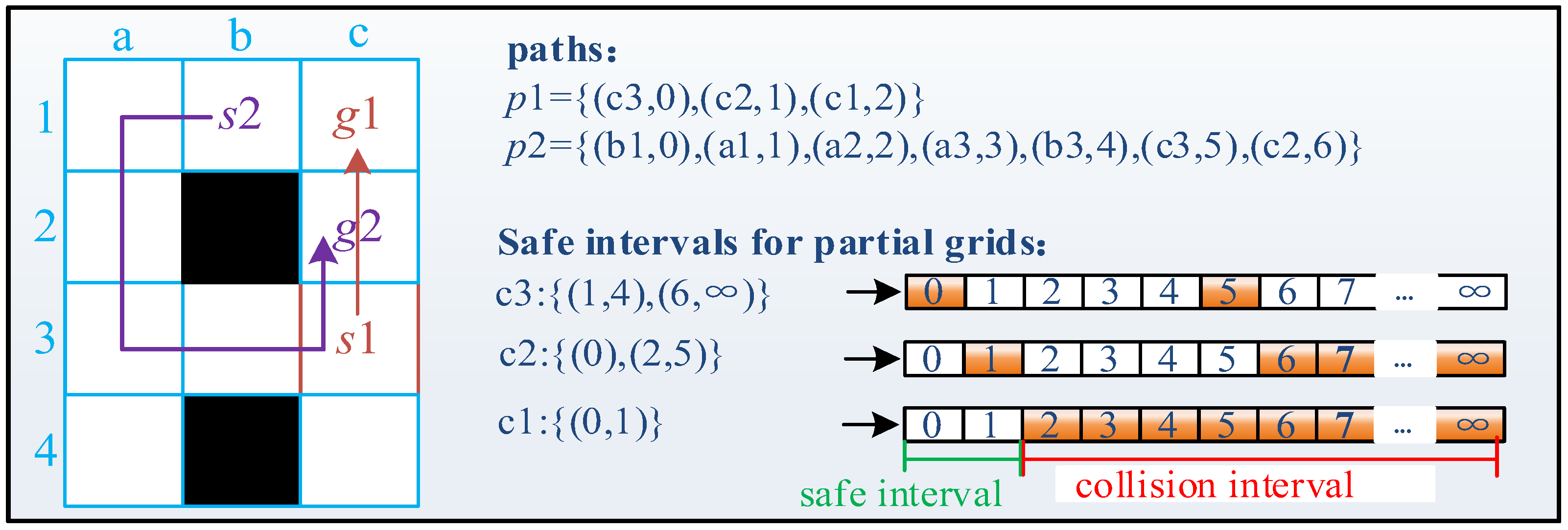
2.1. Basic Principles of the SIPP and CBS Algorithms

As depicted in Figure 1, the SIPP algorithm assigns a safety interval list to each map grid, which records the agent’s occupancy information. When an agent expands into these grids, it directly consults the safety interval list to determine whether the grid can be occupied and the earliest possible time for occupation. The introduction of safe intervals significantly enhances the algorithm’s search efficiency.

As shown in Figure 2, the CBS plans collision-free paths through a conflict-based search tree. Conflict detection is performed between every pair of agents. When a conflict is detected, the search tree splits at the conflicting location, adds constraints to the nodes, and replans the path for one of the agents. This process is repeated until collision-free paths are obtained for all the agents.

2.2. Research Progress on Multi-Agent Collaboration

In today’s society, efficient task execution increasingly relies on sophisticated planning and collaboration within multi-agent systems [26,27]. Wang’s team [28] addressed the challenge of cooperative operation planning in unmanned farms [29] by integrating priority queues with the Dijkstra algorithm [30], achieving efficient path planning. Chen et al. [31] optimized paths for swarm unmanned aerial vehicle (UAV) reconnaissance tasks using a fast evolutionary programming genetic algorithm. Li’s team [32] proposed the adaptive multi-population particle swarm optimization (AMP-PSO) algorithm to shorten paths for multi-AUV (Autonomous Underwater Vehicle) cooperative missions on the seabed. In complex environments, Zhang et al. [33] introduced the multi-objective particle swarm optimization algorithm with multi-mode collaboration based on reinforcement learning (MCMOPSO-RL), which optimizes multi-UAV collaborative paths and effectively handles constraints. Atia et al. [34] designed the Obstacle Guided Path Refinement (ORPG) algorithm to enable air–ground cooperation between UAVs and ground agents. However, these studies primarily focused on small-scale agents and tended to plan independently.

When tackling complex path planning tasks for large-scale agent systems, Grenouilleau et al. [35] built upon the multi-agent pickup and delivery (MAPD) problem [24] by proposing the multi-label A* (MLA*) algorithm, where an agent sequentially visits multiple goal locations, significantly enhancing solution efficiency. However, this study did not involve multi-agent collaboration. Atzmon et al. [36] addressed the multi-agent rendezvous problem with the Meet in the Middle (MM*) algorithm by finding optimal meeting points for multiple agents. Motes et al. [37] combined task decomposition with task planning, introducing the Task and Motion Planning Conflict-Based Search (TMP-CBS) algorithm to handle more complex path-planning problems. Li Jiaoyang et al. [38] proposed the Rolling-Horizon Collision Resolution (RHCR) algorithm for continuous tasks, providing an effective solution for lifelong multi-agent path-finding problems.

Other scholars are actively exploring planning methods for multi-agents collaborating on a single complex task [39,40,41]. However, their research often focuses on path planning within a single cooperative group, neglecting collaboration among multiple cooperative agent groups. Collaborative path planning for multiple agent groups encompasses the following scenarios: (1) Multiple mobile charging agents replenish energy-depleted working agents, reducing travel time and energy consumption to fixed charging areas. (2) In MAPF scenarios, agent paths are optimized through deep collaboration to address path overlaps, minimize travel ranges, and reduce conflicts. (3) In warehouses, multiple sub-task agents collaborate at different workstations to deliver goods to transport agents jointly. To address the complex challenges of collaborative path planning for multiple agent groups, Greshler innovatively introduced the Co-CBS algorithm and systematically established the problem framework of Cooperative Multi-Agent Path Finding (Co-MAPF) for the first time [25]. However, given that research in the Co-MAPF field is still in its infancy, current Co-CBS algorithms mostly focus on simple collaboration scenarios involving two agents, struggling with scenarios involving multiple agents cooperating on complex tasks. The sharp contrast between the aforementioned diverse application requirements and the limitations of current research underscores the necessity and urgency of deepening the research on path planning for multi-group cooperative agents.

3. Problem Description

3.1. MAPF Definition

MAPF Problem Definition: In a given undirected graph $G$ = ($V$, $E$), we have a collection of agents $A$ = {$a_i$ | 0 < $i$ ≤ $N_{robot}$}, where each agent $a_i$ is required to plan a collision-free path $p_i$ from a particular starting point $s_i$ to a goal point $g_i$. Figure 3 shows a schematic representation of a MAPF problem. The starting and goal points are unique for each agent, and the path $p_i$ is represented as a series of grid node and time combinations, i.e., $p_i$={($v_I$, $t_I$) | $I$= 0,1, 2..., ${cost}_i$)}, where ${cost}_i$ represents the time cost required for the agent $a_i$ to move from the starting point to the goal point.

When planning these paths, we must ensure that each agent’s chosen path satisfies Equations (1)–(3) to avoid agents entering obstacle regions or having point conflicts or edge conflicts with other agents. Equation (1) indicates that at any time point $t_I$, no two agents can occupy the same node (point conflict). Equation (2) indicates that at any time point $t_I$, no two agents can traverse the same edge at the same time (edge conflict). Equation (3) requires that each node $v_I$ in the path does not belong to the obstacle region to avoid collision. By satisfying these conditions, we can ensure that all agents can move safely and efficiently from their respective starting points to the goal point while avoiding any collision.

$$\mathrm{s}.\mathrm{t}. p_i\cap p_j=\varnothing i,j \in [1,N_{\mathrm{r}\mathrm{o}\mathrm{b}\mathrm{o}\mathrm{t}}]$$

(1)

$$\{v_I=v_{J-1}\}\cap \{v_J=v_{I-1}\}=\varnothing , v_I\in p_i, v_J \in p_{j}I \in [0,{cost}_i], J \in [0,{cost}_j]$$

(2)

$$v_I \notin obstacles v_I \in p_i, I \in [0,{cost}_i]$$

(3)

The optimization objective of the MAPF problem, as shown in Equation (4), is to minimize the total cost ($flowtime$), which is the sum of the time steps required for each agent to complete its respective task. When agents require little or no waiting, the $\mathrm{f}\mathrm{l}\mathrm{o}\mathrm{w}\mathrm{t}\mathrm{i}\mathrm{m}\mathrm{e}$ value can effectively reflect the quality of the solution.

$$flowtime=min\{\sum _{j=1}^{{k·N}_{group}}{cost}_j+\sum _{i=1}^{N_{group}}{cost}_i\}$$

(4)

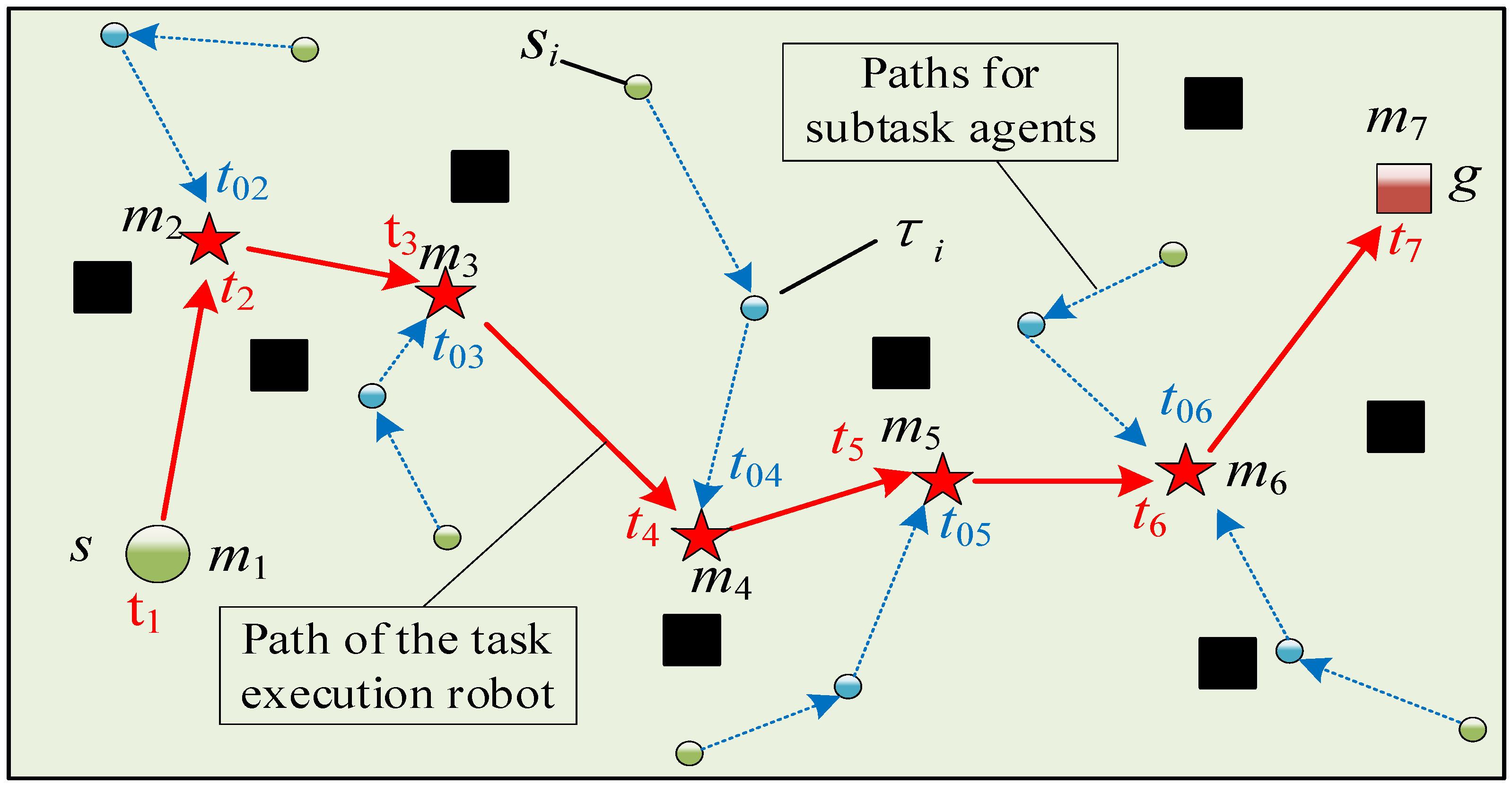
3.2. Co-MAPF Description

3.2.1. Co-MAPF Definition

Co-MAPF Problem Definition: In the context of MAPF, the agents in the agent set $C$ = {$C_i$|0 < $i$ ≤ $N_{group}$} work together to accomplish the tasks $task{s}_i$ within their respective collaborative groups through a $k$-to-1 collaboration model. Each collaborative group $C_i$ consists of $k$ sub-tasking agents and 1 task-executing agent, i.e., $C_i$ = {(($a_{j1}$, $a_{j2}$..., $a_{jk}$), $b_j$)}, where ($a_{j1}$, $a_{j2}$..., $a_{jk}$) represents the $k$ sub-task agents and $b_j$ represents the task execution agent. The collaborative task ${task}_i$ = {(${\tau }_1$, ${\tau }_2$..., ${\tau }_k$), $g$}, where (${\tau }_1$, ${\tau }_2$..., ${\tau }_k$) is the starting point of each sub-task agent and $g$ is the common task goal point.

Taking collaborative distribution as an example, the sub-task agents start from the initial position $s_i$, arrive at the corresponding sub-task position ${\tau }_i$ to obtain the goods and then arrive at the meeting point $m_i$ to carry out the handover of the goods with the task execution agents. After all the sub-task agents complete the handover of the goods, the task execution agent delivers these goods to the final goal point $g$.

For the Co-MAPF problem, the core of the solution lies in planning collision-free paths for sub-task and task-executing agents under the constraints of the MAPF. Considering the difference between the Co-MAPF problem and the general MAPF problem regarding agent behavior during task execution, the task-executing agents need to reach the task handover location and complete the task handover with the sub-task agents before moving to the goal location. Using $flowtime$ as the optimization objective poses the following issues: First, all permutations and combinations of task handover locations and handover times lead to the need to consume a large amount of computational resources to obtain the least time-costly task meeting point, which makes it difficult to provide timely and effective solutions in complex scenarios. Furthermore, optimizing with $flowtime$ as the objective tends to result in longer paths, higher energy consumption, and reduced task volume due to frequent charging, ultimately impacting overall efficiency. Therefore, this paper adopts the total path length ($length$) as the primary optimization objective, as shown in Equation (5) (${pathlength}_i$ is the path of agent $i$), aiming to find a solution with a shorter total length of paths for all agents. This approach aims to reduce energy consumption during actual execution and enhance the system’s overall efficiency.

$$length=min\{\sum _{j=1}^{{k·N}_{group}}{pathlength}_j+\sum _{i=1}^{N_{group}}{pathlength}_i\}$$

(5)

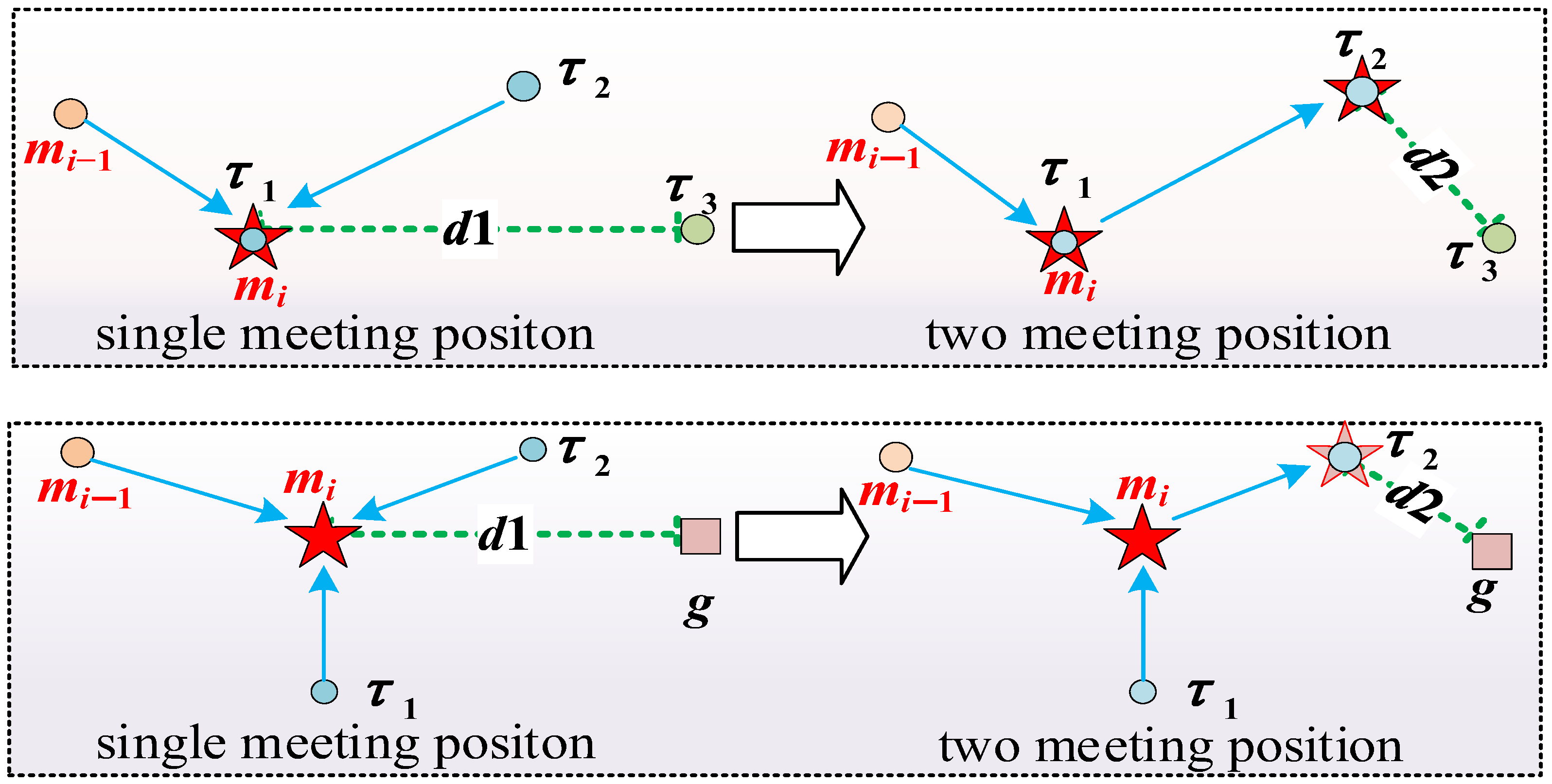
3.2.2. Two Forms of Collaborative Task Handover

When addressing the Co-MAPF problem, the variability of task handover locations and the number of these locations (meeting points) significantly impact the planning outcomes. Therefore, selecting an appropriate strategy to determine the optimal number of meeting points is crucial for obtaining high-quality solutions.

As shown in Figure 4, when adopting the collaboration form with a single meeting point, each set of cooperative task agents must reach a unique meeting point for their group to perform task handovers. This handover form is simple and direct, requires few computational resources, and can be solved using the Cooperative Dynamic Priority SIPP with a single meeting point (Co-${\mathrm{D}\mathrm{P}\mathrm{S}\mathrm{I}\mathrm{P}\mathrm{P}}_{\mathrm{s}}$) algorithm.

However, using a single meeting point for all task handovers can result in some sub-task agents needing to carry tasks and travel longer distances to reach point $m$, where the tasks are then transferred to the final destination point $g$, generating longer redundant paths. Therefore, a better solution can be obtained by adopting the collaboration form with multiple meeting points for task handovers, as illustrated in Figure 5. Naturally, the computational process for multiple meeting points is more complex than for a single one. This problem can be solved using the Cooperative Dynamic Priority SIPP with multiple meeting points (Co-${\mathrm{D}\mathrm{P}\mathrm{S}\mathrm{I}\mathrm{P}\mathrm{P}}_{\mathrm{m}}$) algorithm.

Considering the characteristics of single-meeting-point and multi-meeting-point solving modes, this paper proposes a Cooperative Dynamic Priority SIPP with a multi-meeting-point and single-meeting-point solving mode switching (Co-${\mathrm{D}\mathrm{P}\mathrm{S}\mathrm{I}\mathrm{P}\mathrm{P}}_{\mathrm{m}\mathrm{s}}$) algorithm. The algorithm combines the advantages of both multi-meeting-point and single-meeting-point solving modes, allowing the algorithm to switch to single-meeting-point solving mode when the multi-meeting-point solving mode is in trouble. This approach enhances the algorithm’s success rate and meets the demands of complex collaborative tasks.

4. Co-DP${\mathbf{S}\mathbf{I}\mathbf{P}\mathbf{P}}_{\mathbf{m}\mathbf{s}}$ Algorithm

Given the NP-hard nature of the Co-MAPF problem [42], producing effective paths within a limited time frame is often challenging using optimal algorithms directly in complex environments. Consequently, researchers have shifted their focus to exploring suboptimal algorithms [16,19,20,21], aiming to obtain suboptimal solutions that meet system requirements rapidly. Building upon SIPP as the fundamental path-planning strategy, this paper innovatively proposes a suboptimal path-planning algorithm that achieves efficient collaboration at multiple or single meeting points, thereby swiftly outputting optimized path solutions.

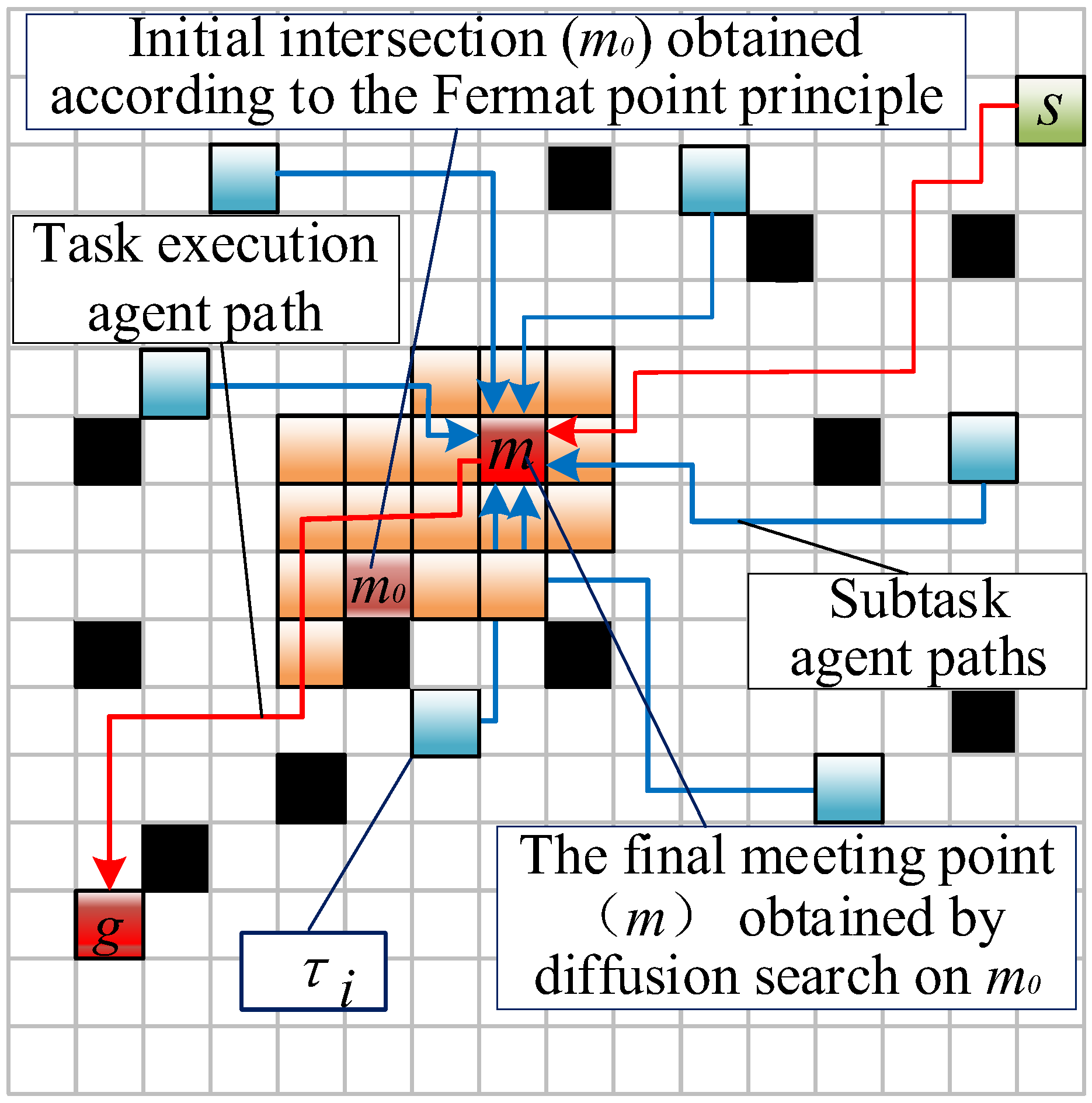
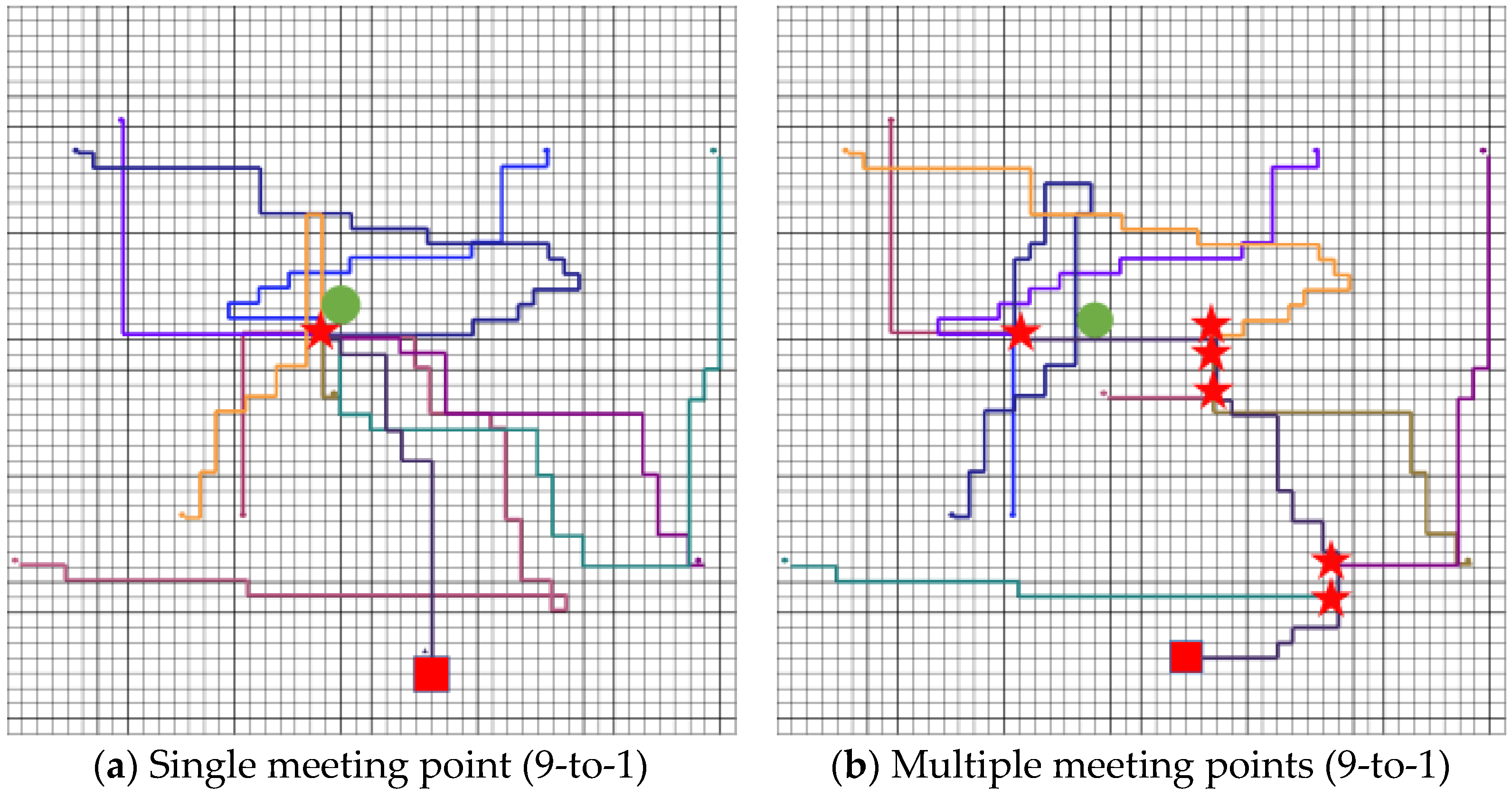
4.1. Multiple Meeting Points Solution Method Considering Obstacles

In the research methodology of this paper, whether it is solving for a single meeting point or a meeting point within a specific subgroup of multiple meeting points, we utilize the principle of the Fermat point to determine an initial meeting point $m_0$ to narrow the search space and then quickly locate the final meeting point $m$ through a grid search in the neighborhood of $m_0$. We refer to this method as the improved Fermat point method. The core idea of the Fermat point principle is to find a point that minimizes the sum of the distances to $N$ known coordinate points; this point is the Fermat point, as shown in Equation (6):

$$min\sum d=\sum _{i=1}^N\sqrt{{(x_0-x_i)}^2+{(y_0-y_i)}^2}$$

(6)

As shown in Figure 6, to obtain the meeting point $\mathrm{m}$ with the shortest total path length, we first input all relevant task coordinate points and quickly calculate an initial reference task intersection point $m_0$ using the Fermat point method. Subsequently, we invoke the underlying path-planning algorithm to plan the paths from all involved task coordinate points to $m_0$ and calculate the total length of these paths, denoted as ${Length}_0$, which serves as the reference path length value. Then, we further plan the paths from these task coordinate points to all neighboring grid cells $v_i$ of $m_0$ and compute the corresponding total path length ${Length}_{vi}$. As shown in Equation (7), if ${Length}_{vi}$ ≤${Length}_0$, we set $m_0$ = $v_i$ and ${Length}_0$ = ${Length}_{vi}$. This process is repeated until all ${Length}_{vi}$ > ${Length}_0$, at which point we set $m$ = $m_0$. Ultimately, we utilize the improved Fermat point method to obtain the task-meeting point $m$ with the shortest total path length.

$$m_0=\left\{\begin{array}{c}{v}_i \exists {Length}_{vi} \le {Length}_0 \\ m_0 \forall {Length}_{vi}>{Length}_0\end{array}\right.$$

(7)

The solution may involve determining multiple meeting points in collaboration with multiple meeting points. In this case, we implement different strategies based on the number of agents within the cooperative group. When the number of agents in a single cooperative group $n$ = 2 and the number of meeting points $N_m$ = 1, then the determination of the meeting point is similar to that shown in Figure 6, using the improved Fermat point method directly. However, when the number of collaborative agents in a single group $n$ > 2, the number of convergence points $N_m$ ∈ [1, n − 1] and the number of agents in a single collaborative group n is determined by a combination of factors such as the task size, the scenario, and the map size. We need to follow these steps to solve multiple meeting points:

(1) First, we collect the position information of each sub-task starting point ${\tau }_i$, the starting point $s$ of the execution agent, and the task destination point $g$.

(2) Next, we connect the starting point $s$ of the execution agent and the task destination point $g$ to form the line segment $L_{sg}$. Then, we calculate the foot of the perpendicular from each sub-task starting point ${\tau }_i$ to the line segment $L_{sg}$, denoted as $f_{ci}$. As shown in Equation (8), based on the relative position of the horizontal coordinate of the foot of the perpendicular $f_{ci}$ to the line segment $L_{sg}$, we divide the corresponding sub-tasks into three parts: pre-segment, intra-segment, and post-segment. In Equation (8), $d_{sf}$ is the distance between point $s$ and point $f$. Notably, in the particular case where the line segment $L_{sg}$ is vertical, the division into three parts is based on the relative position of the vertical coordinate of the foot of the perpendicular $f_{ci}$ to the line segment $L_{sg}$.

$$T_{part}=\left\{\begin{array}{c}1 d_{sf}+d_{gf}>d_{sg} \mathrm{and} d_{sf}<d_{gf}\\ 2 d_{sf}+d_{gf}=d_{sg} \\ 3 d_{sf}+d_{gf}<d_{sg} \mathrm{and} d_{sf}>d_{gf}\end{array}\right.$$

(8)

(3) For sub-task points of the pre-segment, we input their coordinates together with the starting point $s$ of the execution agent and use the improved Fermat point method to solve for the nearest meeting point $p_s$, as shown in the green box on the left side of Figure 7.

(4) For the sub-task points of the post-segment, we input their coordinates together with the task destination point $g$ and utilize the improved Fermat point method to solve for the nearest meeting point $p_g$ to these points, as illustrated in the blue box on the right side of Figure 7.

(5) The process for determining the meeting points of the intra-segment is relatively complex. First, we sort the horizontal coordinates of the feet of the perpendiculars corresponding to the sub-task points (${\tau }_{0i}$) within the segment in ascending order using the bubble sort algorithm, ensuring that the feet closer to point $s$ are ranked higher. This gives us an initial priority order for the agents within the segment. Subsequently, we adjust the starting order of the sub-task agents according to this priority order to accurately determine the meeting points in subsequent calculations.

(6) After ordering adjustment, the sub-task points need to be paired into $\mathrm{q}$ subgroups. As shown in Equation (9), if the number of sub-task points ($N_{{\tau }_0}$) is odd, and a post-segment meeting point $p_g$ exists, we place the last sub-task points ${\tau }_{0k}$ and $p_g$ into the last subgroup (${SG}_q$). If $p_g$ does not exist, we place ${\tau }_{0k}$ and the task destination point $g$ into a subgroup.

$${SG}_q=\left\{\begin{array}{c}\{{\tau }_{0k},p_g\} N_{{\tau }_0}/2=1 \mathrm{and} p_g Exist=True\\ \{{\tau }_{0k},g\} N_{{\tau }_0}/2=1 \mathrm{and} p_g Exist=False\end{array}\right.$$

(9)

(7) After sequencing adjustment, the first sub-task point in the ith subgroup within the same time segment is denoted as ${\tau }_{i1}$. As shown in Figure 8, we use $p_s$ or $s$ (if $p_s$ does not exist) to determine the first meeting point $m_{11}$ of the first subgroup within the segment. Then, using $m_{11}$, ${\tau }_{11}$, and ${\tau }_{12}$, we calculate the second meeting point $m_{12}$ of this subgroup. Following the same principle, we compute the two meeting points $m_{i1}$ and $m_{i2}$ for each remaining subgroup within the segment. If the second coordinate of the last subgroup is $p_g$ or $g$, then the meeting point is $m_{q2}$ = $p_g$ or $m_{q2}$ = $g$, respectively. Otherwise, $m_{q2}$ is calculated using $p_g$ or $g$ (if $p_g$ does not exist) along with ${\tau }_{q1}$ and ${\tau }_{q2}$. Finally, all the computed meeting points within the segment are stored in the meeting point list ${Task}_L$.

(8) After solving all subgroup meeting points, if $p_s$ and $p_g$ exist, they are inserted at the beginning and end of ${Task}_L$, respectively. Subsequently, the task goal point $g$ is added to the end of ${Task}_L$. Finally, the ith meeting point in ${Task}_L$ is defined as $m_i$, which is used in subsequent segmented path planning.

Several vital points need to be explained here: First, during the solving process for the meeting points, we do not directly involve the starting point $s_i$ of the sub-task agent, as the path from $s_i$ to the sub-task starting point ${\tau }_i$ can be planned directly and independently of the meeting points. Second, the pre-segment, intra-segment, and post-segment categorization of sub-task points, along with the priority adjustment of intra-segment sub-task points, ensures that the task-executing agent can perform task handovers with sub-task agents from nearby to far, minimizing redundant paths. Finally, as depicted in Figure 8 and Figure 9, each subgroup is designed with two meeting points, and the meeting points of the preceding subgroup directly participate in the calculations of the subsequent subgroup, enhancing interconnectivity, shortening path lengths, and improving efficiency and performance.

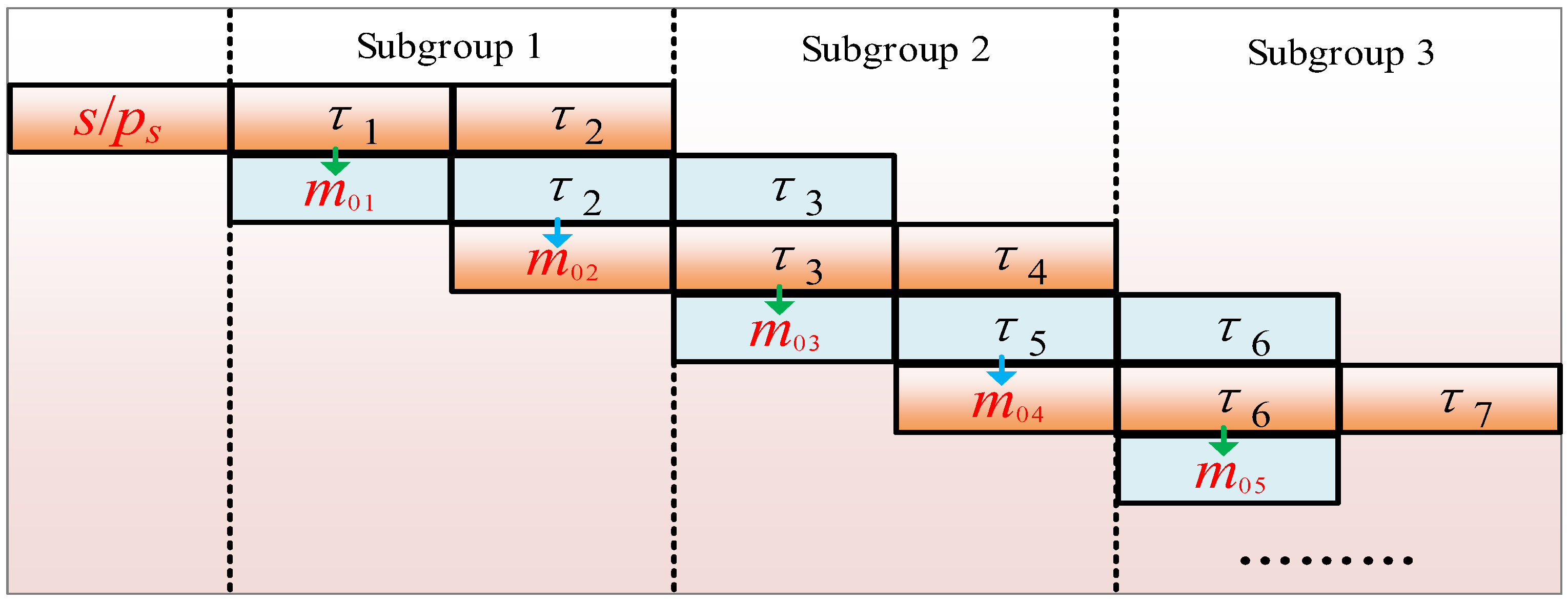
4.2. Segmented Path Planning Strategy

As illustrated in Figure 10, to ensure that each group of collaborative agents efficiently and accurately completes task handovers at their respective meeting points, we implement segmented path-planning strategies explicitly tailored for sub-task agents and task execution agents in terms of setting and planning goal points in the following way. During the prioritization process of planning collaborative task handover paths for sub-task agents, once a sub-task agent reaches its initial goal point (i.e., the starting point of the sub-task, ${\tau }_i$), its goal point is immediately updated to the corresponding final goal point (i.e., the meeting point, $m_i$).

After completing the segmented path planning for each sub-task agent within the collaborative group, it is necessary to compile the arrival time $t_{0i}$ (Equation (10)) of the last agent to reach each meeting point, which will then be utilized in the planning process for the task execution agent.

$$t_{oi}=\mathrm{m}\mathrm{a}\mathrm{x}\left\{{\sum }_{i=1}^{N_{\tau 0}}{\pi }_i\right\}$$

(10)

The complexity of planning collaborative task handover paths for the task execution agent escalates due to the interplay of multiple meeting points. To ensure a smooth transition of tasks, we must factor in the latest arrival time $t_{0i}$ recorded in (1) for sub-task agents at their respective meeting points. As the task execution agent plans routes to these meeting points $m_i$, it compares its estimated arrival time $t_i$ with $t_{0i}$. As shown in Equation (11), if $t_i$ is greater than or equal to $t_{0i}$, indicating that all sub-task agents have arrived, the task execution agent will wait for one time step to facilitate the task handover with the arrived sub-task agents, followed by replacing its goal point. Conversely, if $t_i$ is less than $t_{0i}$, signifying that the task execution agent has reached the meeting point ahead of the sub-task agents, it will execute a waiting operation until $t_i$ equals $t_{0i}$+1 before proceeding with the goal point replacement.

$$t_{wait}=\left\{\begin{array}{c}1 t_i\ge t_{0i} \\ t_i-t_{0i}+ 1 t_i<t_{0i}\end{array}\right.$$

(11)

By adopting this clear and well-defined segmented path planning strategy, we ensure the orderliness and efficiency of the collaborative agents during task execution, thereby minimizing confusion and delays in the task handover process.

4.3. Hybrid Solution Mode Switching Mechanism

When utilizing a collaborative path planning approach with multiple meeting points, while it can offer optimization in path length, in certain specific scenarios, the numerous and dispersed handover points within the movement-constrained areas of the map can make it exceedingly challenging, if not impossible, to identify and reach these meeting points, potentially leading to solution failure. In such cases, the more straightforward and more direct approach of solving for a single meeting point may paradoxically have a greater chance of successfully finding a solution. Consequently, this paper proposes an intelligent switching strategy that integrates both the multi-meeting-point and single-meeting-point solving modes. The aim is to prioritize ensuring the algorithm’s success rate while also optimizing the path length. As depicted in Equation (12) and Figure 11, the algorithm initially attempts to solve problems using the multi-meeting-point solving mode ($MMP$). If the solving time in this mode $t$ ≥ 1/6$·T_0$ and the number of solving failures in the multi-meeting-point solving mode$c$ ≥ 1, the algorithm automatically switches to the single-meeting-point solving mode ($SMP$). Even in this simplified mode, if the solution remains elusive, the algorithm continues to seek a solution by adjusting the group priorities. The solution complexity is higher in the multi-meeting-point solving model because a collaborative group needs to solve for multiple meeting locations. In contrast, a collaborative group only needs to solve for one meeting location in the single-meeting-point solving model, which has a lower solution complexity in comparison. However, the path solution obtained by all agents performing task handover at a single meeting point produces redundant paths that are longer and consume more energy to move than performing task handover at multiple meeting points. Therefore, the multi-meeting-point solving model is preferred for solving when conditions allow one to obtain a better path scheme.

$$MD=\left\{\begin{array}{c}MMP t<1/6·T_0 \mathrm{or} c<1 \\ SMP t\ge 1/6·T_0 and c\ge 1 \end{array}\right.$$

(12)

In addition, two prioritization methods are used in this paper to obtain better optimal solutions and higher success rates. In the multi-meeting-point solving mode, the algorithm performs priority adjustments within individual collaborative groups to ensure the task execution agent can hand over tasks with sub-task agents in an optimal sequence, thereby reducing unnecessary path redundancy. For the entire multi-agent system, priority adjustments focus on the entire group, aiming to enhance the success rate of the solution by optimizing interactions between groups. The group prioritization adjustment method is shown in Equation (13), where $P_{Gi}$ is the group priority of ${group}_i$ and $P_{GF}$ is the priority of the group where the solution failed:

$$P_{Gi}=\left\{\begin{array}{c}1 P_{Gi}=P_{GF} \\ i+1 P_{Gi}<P_{GF}\\ i P_{Gi}>P_{GF}\end{array}\right.$$

(13)

4.4. Pseudocode and Flowchart of the Co-${DPSIPP}_{ms}$ Algorithm

The pseudocodes for the Co-${\mathrm{D}\mathrm{P}\mathrm{S}\mathrm{I}\mathrm{P}\mathrm{P}}_{\mathrm{m}\mathrm{s}}$ algorithm are presented in Algorithms 1 and 2. Algorithm 1 is the planning system’s upper layer and is responsible for priority adjustments, solving mode switching, and safety interval updates. Algorithm 2, conversely, constitutes the lower layer of the planning system, tasked with segmenting and planning collision-free paths for individual agents.

Algorithm 1: Co-${\mathrm{D}\mathrm{P}\mathrm{S}\mathrm{I}\mathrm{P}\mathrm{P}}_{\mathrm{m}\mathrm{s}}$ algorithm

input:         $Group=\{\dots ,{group}_i=\left({agents}_a,{agent}_b,{task}_i\right),\dots \}, \mathrm{M}\mathrm{a}\mathrm{p},T_0,MD=MMP$ %$MD=MMP$, initial use of multi-meeting-point solving mode

output:$Paths,length$

1: while $t$ <$T_0$ do

2:  for ${group}_i$ in Group do

3:    if $MD$=$MMP$ then

4:     $newGoa\mathrm{l}{\leftarrow M}_{i1}$←CalMultipleMeetingPoints(${group}_i$)          %Solving for multiple meeting points

5:    end if

6:    if $MD$ = $SMP$ then

7:     $newGoal{\leftarrow M}_{i2}$←CalSingleMeetingPoint(${group}_i$)        %Solving for single meeting point

8:    end if

9:    for $\mathrm{a}\mathrm{g}\mathrm{e}\mathrm{n}\mathrm{t}$ in ${group}_i$ do

10:     $res, {path}_i$←$\mathrm{i}\mathrm{S}\mathrm{I}\mathrm{P}\mathrm{P}$($agent,id,Map,newGoal)$

11:     if $res=successful$ then

12:      ${path}_i$ insert $Paths$, update $SafeInterval$        %Update safe intervals to avoid future conflicts

13:     end if

14:     if $res=failed$ then

15:      if $MD$ = $MM$P and $t$ ≥ 1/6∙$T_0$ then

16:        $MD$ =$M$SP

17:      end if

18:      $newGroup$←DeterReScheduling(${group}_i,Group$)         %Set the priority of failed groups to the highest

19:      $Group$←$newGroup$

20:      $Paths$←$\mathrm{\varnothing }$,$Safe\_interval$←$InitialSafeInterval$

21:     end if

22:    end for

23:  end for

24:  return $Paths$, $length$

25: end while

26: return $,\mathrm{\varnothing },0$

Algorithm 2: iSIPP algorithm

input:$agent, id,Map,newGoal$,$Replaced$=$False$

output:$\mathrm{p}\mathrm{a}\mathrm{t}h$

1: while $curNode\ne agentGoal$ do

2:  expand nodes using A*

3:  if OPEN = $\mathrm{\varnothing }$ then

4:    return $failed,\varnothing$

5:  end if

6:  if not $Replaced$ then

7:   if $curNode=agentGoal$ then

8:     if $agent$ is ${agent}_b$ then

9:       Perform the wait operation according to Equation (11)

10:    end if

11:    $agentGoal={newGoal}_{id}$      %A unvisited meeting location as new goal point

12:    if ${newGoal}_{id}$ is $agentFinalGoal$ then

13:    $Replaced=True$ %Plan to the ultimate goal

14:    end if

15:   end if

16:  end if

17:  if $Replaced$ then

18:   if $curNode=agentGoal$ then

19:     return $successful, path$

20:   end if

21:  end if

22: end while

Figure 12 details the complete flow of the Co-${\mathrm{D}\mathrm{P}\mathrm{S}\mathrm{I}\mathrm{P}\mathrm{P}}_{\mathrm{m}\mathrm{s}}$ algorithm, which comprises six crucial components: meeting point solving, segmented path planning, global safety interval updating, switching between multi-meeting-point and single-meeting-point solving modes, and group priority adjustments. These components work in concert to ensure that the algorithm can optimize the path length and efficiency of task execution while guaranteeing a high success rate of the solution.

In the Co-${\mathrm{D}\mathrm{P}\mathrm{S}\mathrm{I}\mathrm{P}\mathrm{P}}_{\mathrm{m}\mathrm{s}}$ algorithm, the majority of the computation time is focused on solving for the meeting points. When $N_{group}$ collaborative groups are operating simultaneously, with each group containing $n$ agents and each group requiring $k$ meeting points for task handovers, the solution for each meeting point involves $r$ iterations of the search. Under this scenario, the underlying single-agent path planning algorithm will be invoked $k·r·n{·N}_{group}$ times during the process of solving for the meeting points. As a result, the time complexity of solving all meeting points can be expressed as follows:

$$O(Time)={k·r·N}_{group}\sum _{i=0}^n{O\left(b\right)}^{T_i}$$

(14)

In Equation (14), $b$ represents the number of states that the algorithm can expand outward during the node expansion process, $T_i$ denotes the length of the path for a single agent (as a measure of path search complexity), and $\sum _{i=0}^n{O\left(b\right)}^{T_i}$ represents the time complexity of formally planning the path once all goal points are known. Due to the need to repeatedly invoke the underlying path planning algorithm while solving for meeting points, the time complexity of this part is almost $k·r{·N}_{group}$ times that of formally planning the path. These data show a significant increase in the computational complexity of the Collaborative Multi-Agent Path Finding problem (Co-MAPF) compared to the classical MAPF problem. This increase is primarily attributed to the additional computations and iterative searches introduced by solving for meeting points.

5. Simulation Experimental Analysis

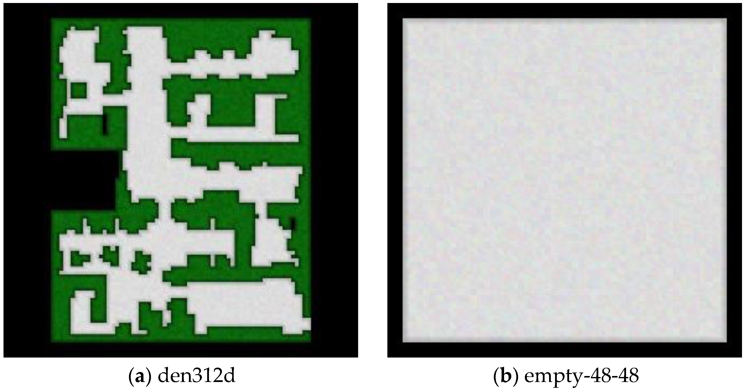
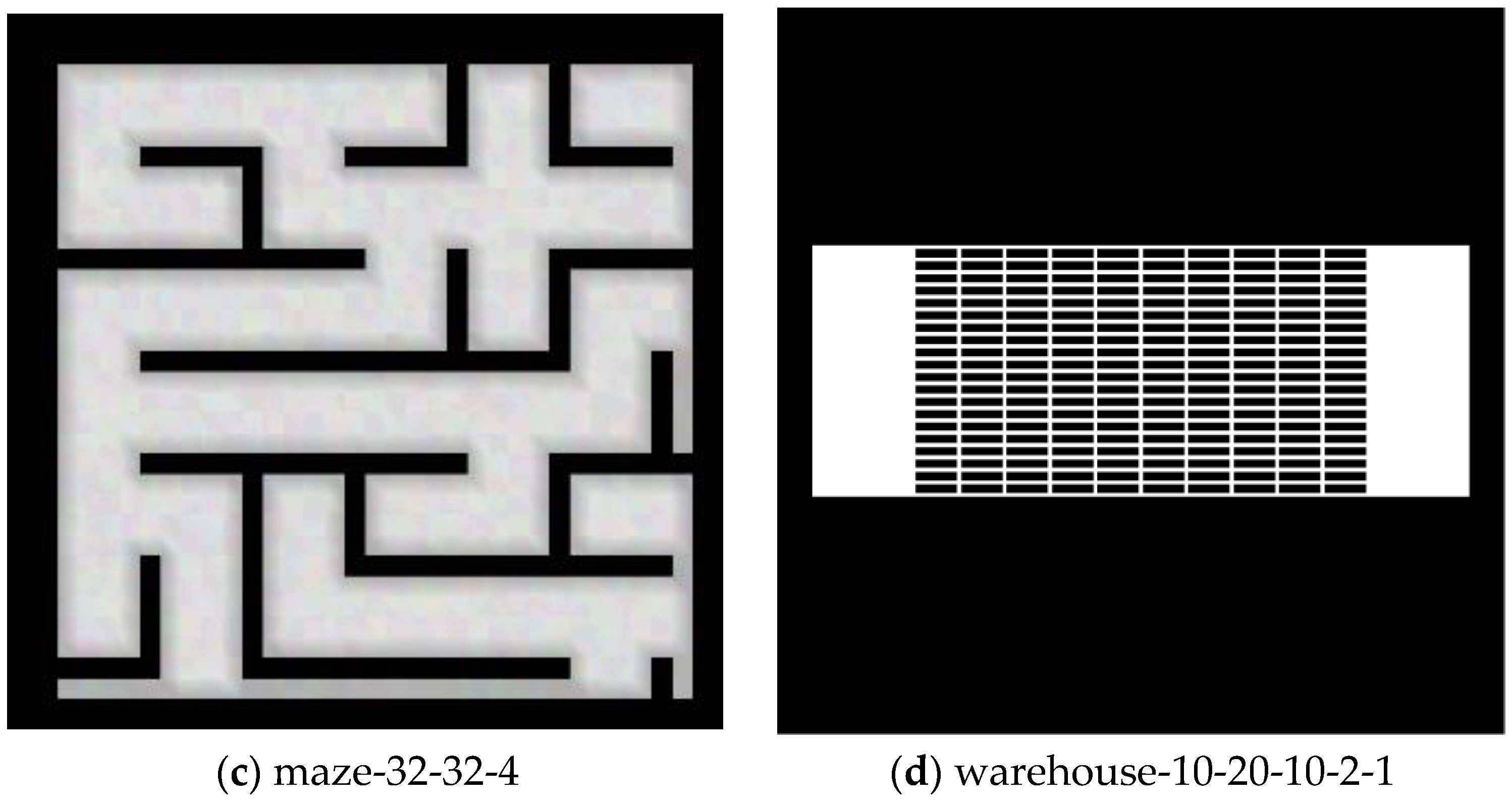
5.1. Experimental Parameter Settings

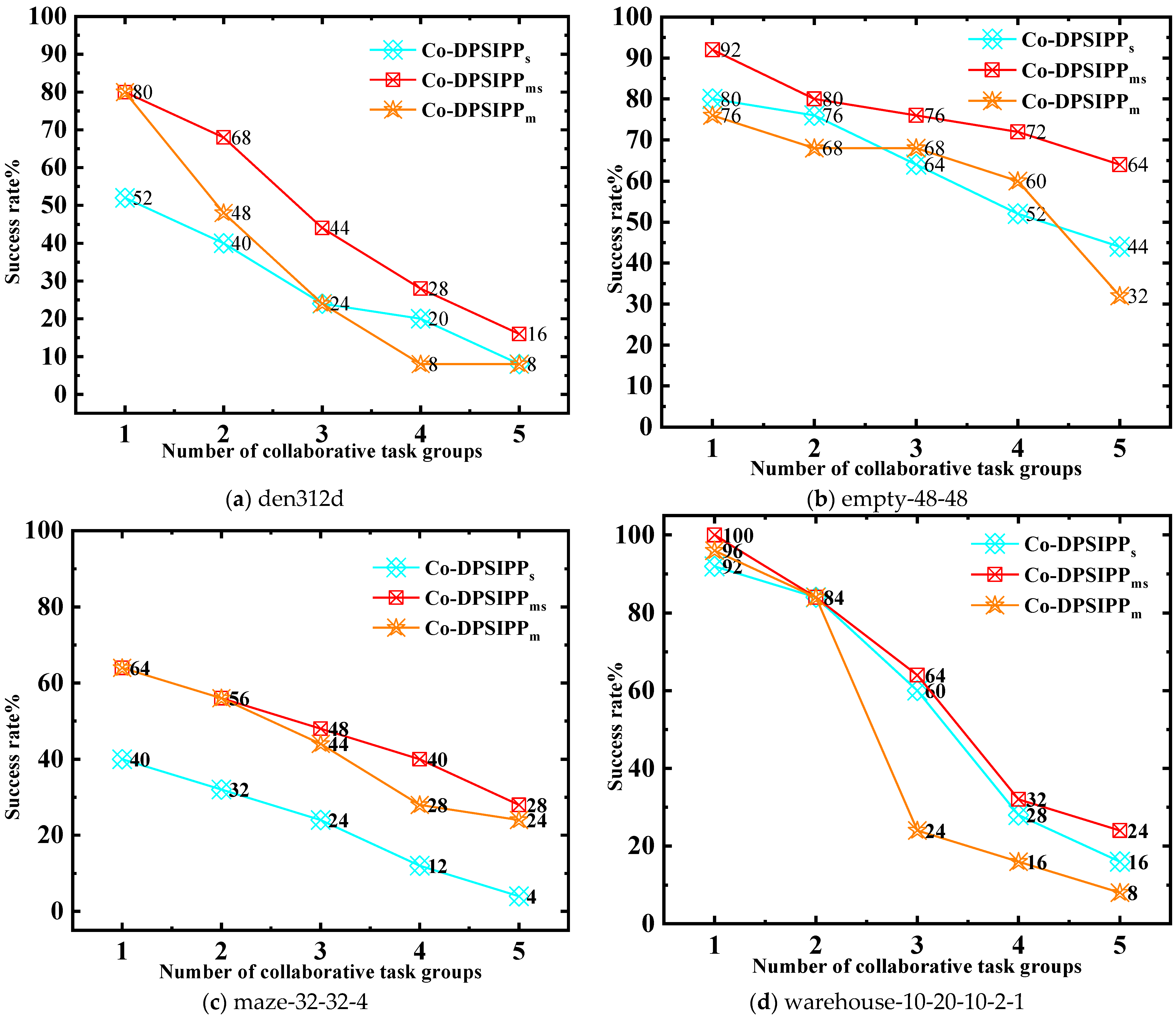
This paper compares the performances of the different collaborative agent path-planning algorithms through three simulation experiments. Simulation Experiment 1 primarily focuses on the performance of the Co-CBS algorithm and the Co-${\mathrm{D}\mathrm{P}\mathrm{S}\mathrm{I}\mathrm{P}\mathrm{P}}_{\mathrm{m}\mathrm{s}}$ algorithm in scenarios where only two agents collaborate. Simulation Experiment 2 provides a more comprehensive evaluation of three algorithms: Cooperative Dynamic Priority SIPP with a single meeting point (Co-${\mathrm{D}\mathrm{P}\mathrm{S}\mathrm{I}\mathrm{P}\mathrm{P}}_{\mathrm{s}}$), Cooperative Dynamic Priority SIPP with multiple meeting points (Co-${\mathrm{D}\mathrm{P}\mathrm{S}\mathrm{I}\mathrm{P}\mathrm{P}}_{\mathrm{m}}$), and Cooperative Dynamic Priority SIPP with multi-meeting-point and single-meeting-point solving mode switching (Co-${\mathrm{D}\mathrm{P}\mathrm{S}\mathrm{I}\mathrm{P}\mathrm{P}}_{\mathrm{m}\mathrm{s}}$). Additionally, Simulation Experiment 3 exemplifies the impact of the number of agents within a single collaborative group on the solution results of both the Co-${\mathrm{D}\mathrm{P}\mathrm{S}\mathrm{I}\mathrm{P}\mathrm{P}}_{\mathrm{s}}$ and Co-${\mathrm{D}\mathrm{P}\mathrm{S}\mathrm{I}\mathrm{P}\mathrm{P}}_{\mathrm{m}\mathrm{s}}$ algorithms.

The experiments were conducted on a Windows 10 PC with an Intel Core i7 (3.6 GHz) CPU and 32 GB of RAM, and the algorithms ran on an Ubuntu 20.04 environment installed on a VMware17 virtual machine to ensure a fair comparison on a unified platform. In order to evaluate the algorithm’s solution efficiency, we set each planning limit time $T_0$ to 5 min. If an algorithm failed to return a valid solution within this time, the corresponding instance was considered a failure.

The experimental maps included standard Nest, Empty, Maze, and Warehouse maps, as shown in Figure 13, simulating environments of varying complexity. For experiments involving $n$ agents within a single collaborative task, we utilized the $n$ sets of coordinates from the instance files (i.e., Scenarios files) accompanying the standard maps to set the starting positions of the agents, sub-task starting points, and task goal points. The starting point and goal point of the first sub-task correspond to the starting and goal points of the first set of coordinates, the starting point of the first sub-task agent and the starting point of the task execution agent correspond to the starting and goal points of the second set of coordinates, and the starting points of the remaining $n$-2 sub-task agents and sub-task starting points correspond to the starting and goal points of the remaining $n$-2 sets of coordinates.

In Simulation Experiment 1, we set the number of agents within a single collaborative group to $n$ = 2. We gradually increased the number of collaborative task groups $N_{group}$ from 6 to 30 to evaluate the performance of the algorithms under different collaboration group sizes. In Simulation Experiment 2, we fixed the number of agents within a single collaborative group to $n$ = 10. We incrementally increased the number of collaborative task groups $N_{group}$ from 1 to 5 to analyze the performance of the algorithms in multi-group collaboration scenarios. To further explore the impact of the number of agents within a single collaborative group on the experimental results, we conducted an additional set of experiments where $N_{group}$=1, and the number of agents within a single collaborative group $n$ was gradually increased from 5 to 25. Each experiment was repeated 5 times, with each test comprising 25 instances, to ensure the reliability and stability of the results. The $runtime$ metric represents the time the algorithm takes to return a valid solution during the solution process, reflecting the algorithm’s solution efficiency. When comparing $runtime$, total path length ($length$), and total path cost ($flowtime$), we took the average values of public solutions as the basis for comparison to more accurately assess the merits of the algorithms. Additionally, we bolded the best-performing data among several algorithms for a more intuitive comparison.

In Figure 14, we present the multi-agent path planning algorithm’s planned paths utilizing multiple and single-meeting-point collaboration formats, and a line of one color denotes a robot’s path. Figure 14a,b corresponds to these two collaboration formats, respectively, involving 9 sub-task agents and 1 task execution agent working together to complete tasks. In the figures, the green circles represent the starting points of the task execution agent, the red rectangles mark the task goal points, and the red five-pointed stars indicate the meeting points calculated by the algorithm. It is evident from the figures that the path in the single meeting-point-collaboration format tends to converge toward a single handover point, leading to longer redundant segments in the path. In contrast, the path in the multi-meeting-point collaboration format allows for task handovers at multiple different handover points, enabling more flexible path planning and significantly reducing the length of redundant paths. This optimization not only improves the overall task execution efficiency but also decreases the energy consumption of agents during task execution.

5.2. Simulation Experiment 1

Figure 15 and

Table 1. Comparison of path solutions between Co-CBS and Co-${\mathrm{D}\mathrm{P}\mathrm{S}\mathrm{I}\mathrm{P}\mathrm{P}}_{\mathrm{m}\mathrm{s}}$ algorithms in 1-to-1 collaboration.

Map	Ngroup	Length/Step		Flowtime/Step		Runtime/s
		Co-${\mathbf{D}\mathbf{P}\mathbf{S}\mathbf{I}\mathbf{P}\mathbf{P}}_{\mathbf{m}\mathbf{s}}$	Co-CBS	Co-${\mathbf{D}\mathbf{P}\mathbf{S}\mathbf{I}\mathbf{P}\mathbf{P}}_{\mathbf{m}\mathbf{s}}$	Co-CBS	Co-${\mathbf{D}\mathbf{P}\mathbf{S}\mathbf{I}\mathbf{P}\mathbf{P}}_{\mathbf{m}\mathbf{s}}$	Co-CBS
den312d	6	768.8	893.9	1014.2	972.7	16.12	43.42
empty-48-48	6	467.88	536.12	665.52	592	4.63	8.47
	12	950.72	1089.94	1253.72	1194.44	17.68	22.29
	18	1426.6	1607.8	1912.2	1777.2	54.29	128.65
maze-32-32-4	6	620.75	636.25	786.5	729.75	28.91	46.89
warehouse-10-20-10-2-1	6	1254.4	1396.93	1630.86	1540.2	10.34	70.71
	12	2379.33	2598.33	3096	2847.33	26.38	156.83

Note: The data marked in bold are the best performing data from the results of the comparison algorithm.

present a comparative analysis of the test results between the Co-CBS algorithm and the Co-${\mathrm{D}\mathrm{P}\mathrm{S}\mathrm{I}\mathrm{P}\mathrm{P}}_{\mathrm{m}\mathrm{s}}$ algorithm when only two agents collaborate. In the 1-to-1 collaboration scenario, as depicted in Figure 15, the Co-${\mathrm{D}\mathrm{P}\mathrm{S}\mathrm{I}\mathrm{P}\mathrm{P}}_{\mathrm{m}\mathrm{s}}$ algorithm demonstrates significant advantages over the Co-CBS algorithm, particularly regarding the solution success rate. Specifically, across four different maps (Nest, Empty, Maze, and Warehouse), the solution success rate of Co-${\mathrm{D}\mathrm{P}\mathrm{S}\mathrm{I}\mathrm{P}\mathrm{P}}_{\mathrm{m}\mathrm{s}}$ improved by 60%, 53.6%, 19.2%, and 24%, respectively, showing remarkable superiority. Furthermore, by comparing the maximum number of solvable collaboration task groups between the two algorithms, we found that Co-${\mathrm{D}\mathrm{P}\mathrm{S}\mathrm{I}\mathrm{P}\mathrm{P}}_{\mathrm{m}\mathrm{s}}$ was able to solve more collaboration task groups on all four maps. Notably, on the Nest and Maze maps, the number of solvable collaboration task groups achieved by Co-${\mathrm{D}\mathrm{P}\mathrm{S}\mathrm{I}\mathrm{P}\mathrm{P}}_{\mathrm{m}\mathrm{s}}$ was more than twice that by Co-CBS. In summary, the Co-${\mathrm{D}\mathrm{P}\mathrm{S}\mathrm{I}\mathrm{P}\mathrm{P}}_{\mathrm{m}\mathrm{s}}$ algorithm boasts a higher solution success rate and handles more collaboration task groups and agent instances on these four maps, demonstrating more robust solving capabilities and adaptability.

Table 1 reveals that the Co-${\mathrm{D}\mathrm{P}\mathrm{S}\mathrm{I}\mathrm{P}\mathrm{P}}_{\mathrm{m}\mathrm{s}}$ algorithm exhibits significant advantages over the Co-CBS algorithm regarding the total path length and algorithm solving time. Specifically, on the Nest, Empty, Maze, and Warehouse maps, the path solutions generated by Co-${\mathrm{D}\mathrm{P}\mathrm{S}\mathrm{I}\mathrm{P}\mathrm{P}}_{\mathrm{m}\mathrm{s}}$ are 13.9%, 12.2%, 2.4%, and 9.3% shorter in total path length, respectively, than those generated by Co-CBS. Concurrently, the solving times are reduced by 62.8%, 41.3%, 38.3%, and 84.2%, respectively. These results imply that the Co-${\mathrm{D}\mathrm{P}\mathrm{S}\mathrm{I}\mathrm{P}\mathrm{P}}_{\mathrm{m}\mathrm{s}}$ algorithm can find path solutions in a much shorter time in addition to maze maps, and the obtained path solutions are able to reduce energy consumption by about 10% compared to the Co-CBS algorithm, which is an essential economic and environmental benefit in practical applications.

However, regarding the total path cost, the Co-${\mathrm{D}\mathrm{P}\mathrm{S}\mathrm{I}\mathrm{P}\mathrm{P}}_{\mathrm{m}\mathrm{s}}$ algorithm is inferior to the Co-CBS algorithm. This is primarily due to the optimization objective of the Co-${\mathrm{D}\mathrm{P}\mathrm{S}\mathrm{I}\mathrm{P}\mathrm{P}}_{\mathrm{m}\mathrm{s}}$ algorithm, which focuses on minimizing the total path length. In some scenarios, to avoid unnecessary energy consumption, the task execution agent may need to wait at the meeting point for the sub-task agents to arrive for task handover, resulting in a higher path cost than the Co-CBS algorithm. Nevertheless, considering the significant advantages of the Co-${\mathrm{D}\mathrm{P}\mathrm{S}\mathrm{I}\mathrm{P}\mathrm{P}}_{\mathrm{m}\mathrm{s}}$ algorithm in terms of path length and solving time, it holds a high application value and potential in multi-agent cooperative path planning.

5.3. Simulation Experiment 2

The planning results of the Co-${\mathrm{D}\mathrm{P}\mathrm{S}\mathrm{I}\mathrm{P}\mathrm{P}}_{\mathrm{s}}$, Co-${\mathrm{D}\mathrm{P}\mathrm{S}\mathrm{I}\mathrm{P}\mathrm{P}}_{\mathrm{m}}$, and Co-${\mathrm{D}\mathrm{P}\mathrm{S}\mathrm{I}\mathrm{P}\mathrm{P}}_{\mathrm{m}\mathrm{s}}$ algorithms, as depicted in Figure 16 and

Table 2. Path solution comparison of the Co-${\mathrm{D}\mathrm{P}\mathrm{S}\mathrm{I}\mathrm{P}\mathrm{P}}_{\mathrm{s}}$ and Co-${\mathrm{D}\mathrm{P}\mathrm{S}\mathrm{I}\mathrm{P}\mathrm{P}}_{\mathrm{m}\mathrm{s}}$ algorithms in the 9-to-1 collaboration.

Map	Ngroup	Length/Step		Flowtime/Step		Runtime/s
		Co-${\mathbf{D}\mathbf{P}\mathbf{S}\mathbf{I}\mathbf{P}\mathbf{P}}_{\mathbf{m}\mathbf{s}}$	Co-${\mathbf{D}\mathbf{P}\mathbf{S}\mathbf{I}\mathbf{P}\mathbf{P}}_{\mathit{s}}$	Co-${\mathbf{D}\mathbf{P}\mathbf{S}\mathbf{I}\mathbf{P}\mathbf{P}}_{\mathbf{m}\mathbf{s}}$	Co-${\mathbf{D}\mathbf{P}\mathbf{S}\mathbf{I}\mathbf{P}\mathbf{P}}_{\mathbf{s}}$	Co-${\mathbf{D}\mathbf{P}\mathbf{S}\mathbf{I}\mathbf{P}\mathbf{P}}_{\mathbf{m}\mathbf{s}}$	Co-${\mathbf{D}\mathbf{P}\mathbf{S}\mathbf{I}\mathbf{P}\mathbf{P}}_{\mathbf{m}}$
den312d	1	760.38	806	852.84	929	21.18	7.86
	2	1433.6	1638.6	1594.4	1860.6	121.37	73.37
	3	2262	2446	2567.5	2765.5	157.45	103.88
	4	2702	3307.5	2920.25	3793.25	233.2	283.64
	5	3190	4083	3433	4613	241.32	300
empty-48-48	1	454.25	495.85	506.15	565.85	2.64	3.05
	2	855.66	1014.44	922.16	1153.33	35.71	26.92
	3	1253.53	1537.33	1363.6	1757.93	39.85	84.91
	4	1653	2076.63	1770.63	2356.81	116.41	213.75
	5	2108.1	2607.44	2284.67	2951.22	213.45	293.93
maze-32-32-4	1	604.9	637.7	727	757.8	19.76	8.92
	2	1213.75	1404.87	1427	1695.87	42.35	25.61
	3	1797.5	2087.5	2152.5	2631.5	80.04	50.82
	4	2612.66	2808	3475.66	3812	149.02	92.46
warehouse-10-20-10-2-1	1	951.3	1113.95	1035.08	1268.91	7.94	4.49
	2	2185.68	2526.36	2373.89	2860.26	65.34	74.71
	3	3689.61	3813.53	4154.53	4295.53	131.82	118.85
	4	5373.2	5523.2	5984	6185.4	212.97	167.66
	5	6632.66	7100.66	7451	7969	259.82	229.61

Note: The data marked in bold are the best performing data from the results of the comparison algorithm.

, provide an insightful comparative analysis. Figure 16 shows that the Co-${\mathrm{D}\mathrm{P}\mathrm{S}\mathrm{I}\mathrm{P}\mathrm{P}}_{\mathrm{m}\mathrm{s}}$ algorithm, which utilizes multiple meeting points, outperforms the Co-${\mathrm{D}\mathrm{P}\mathrm{S}\mathrm{I}\mathrm{P}\mathrm{P}}_{\mathrm{s}}$ algorithm with a single meeting point regarding the solution success rate. Specifically, on the Nest, Empty, Maze, and Warehouse maps, the solution success rates improve by 18.4%, 13.6%, 24.8%, and 4.8%, respectively. This advantage primarily stems from the dual-mode solving strategy employed by the Co-${\mathrm{D}\mathrm{P}\mathrm{S}\mathrm{I}\mathrm{P}\mathrm{P}}_{\mathrm{m}\mathrm{s}}$ algorithm, which combines the strengths of both solving modes. When the multi-meeting-point solving mode encounters challenges, the algorithm can flexibly switch to the single-meeting-point solving mode, thereby enhancing the overall solution success rate.

Furthermore, the data in Table 2 reinforce the superiority of the Co-${\mathrm{D}\mathrm{P}\mathrm{S}\mathrm{I}\mathrm{P}\mathrm{P}}_{\mathrm{m}\mathrm{s}}$ algorithm in path planning. Regarding the average total path length, Co-${\mathrm{D}\mathrm{P}\mathrm{S}\mathrm{I}\mathrm{P}\mathrm{P}}_{\mathrm{m}\mathrm{s}}$ achieves reductions of 13.14%, 16.34%, 10.5%, and 8.12% compared to Co-${\mathrm{D}\mathrm{P}\mathrm{S}\mathrm{I}\mathrm{P}\mathrm{P}}_{\mathrm{s}}$ across the four maps. This significant improvement is attributed to the ability of the Co-${\mathrm{D}\mathrm{P}\mathrm{S}\mathrm{I}\mathrm{P}\mathrm{P}}_{\mathrm{m}\mathrm{s}}$ algorithm to guide the sub-task agents and task execution agents to select more suitable locations on the map for task handover, effectively reducing redundant paths. Co-${\mathrm{D}\mathrm{P}\mathrm{S}\mathrm{I}\mathrm{P}\mathrm{P}}_{\mathrm{m}\mathrm{s}}$ not only decreases the energy consumption of the agentic system but also saves operational costs. The Co-${\mathrm{D}\mathrm{P}\mathrm{S}\mathrm{I}\mathrm{P}\mathrm{P}}_{\mathrm{m}\mathrm{s}}$ algorithm also demonstrates a clear advantage regarding the average total path cost, reducing the total cost by 15.52%, 20.04%, 11.68%, and 9.68% on the four maps, respectively. Regarding algorithm runtime, on the relatively spacious Nest and Empty maps, the Co-${\mathrm{D}\mathrm{P}\mathrm{S}\mathrm{I}\mathrm{P}\mathrm{P}}_{\mathrm{m}\mathrm{s}}$ algorithm, which switches between multiple-meeting-point and single-meeting-point solving modes when $N_{group}$ > 3, can return solutions faster. However, in complex and narrow maps, such as Maze and Warehouse, the Co-${\mathrm{D}\mathrm{P}\mathrm{S}\mathrm{I}\mathrm{P}\mathrm{P}}_{\mathrm{s}}$ algorithm with a single-meeting-point solving mode returns solutions more quickly.

From the above results, it is evident that the Co-${\mathrm{D}\mathrm{P}\mathrm{S}\mathrm{I}\mathrm{P}\mathrm{P}}_{\mathrm{m}\mathrm{s}}$ algorithm performs exceptionally well on the Nest, Empty, and Maze maps, while its advantage diminishes slightly on the Warehouse map with severely restricted mobility. Compared to Co-${\mathrm{D}\mathrm{P}\mathrm{S}\mathrm{I}\mathrm{P}\mathrm{P}}_{\mathrm{s}}$, Co-${\mathrm{D}\mathrm{P}\mathrm{S}\mathrm{I}\mathrm{P}\mathrm{P}}_{\mathrm{m}\mathrm{s}}$ significantly improves the solution success rate, shortens the path length, and reduces the total path cost at the expense of a slightly longer algorithm runtime.

5.4. Simulation Experiment 3

To further investigate the impact of increasing the number of cooperative agents on the performance of the two algorithms, we conducted tests on an obstacle-free empty map, and the results are presented in Figure 17.

By comparing instances where both Co-${\mathrm{D}\mathrm{P}\mathrm{S}\mathrm{I}\mathrm{P}\mathrm{P}}_{\mathrm{s}}$ and Co-${\mathrm{D}\mathrm{P}\mathrm{S}\mathrm{I}\mathrm{P}\mathrm{P}}_{\mathrm{m}\mathrm{s}}$ can find solutions in a single run, we observed that as the number of agents in a single cooperative group increases, the Co-${\mathrm{D}\mathrm{P}\mathrm{S}\mathrm{I}\mathrm{P}\mathrm{P}}_{\mathrm{m}\mathrm{s}}$ algorithm, which employs multiple meeting points, exhibits increasingly significant optimization effects regarding path length and total path cost. This is because, as the number of agents in a single cooperative group increases, the single-meeting-point approach is more prone to generating redundant paths. In contrast, the Co-${\mathrm{D}\mathrm{P}\mathrm{S}\mathrm{I}\mathrm{P}\mathrm{P}}_{\mathrm{m}\mathrm{s}}$ algorithm effectively reduces these redundancies through the multi-meeting-point approach. However, when the number of agents reaches a certain threshold, the optimization effect tends to stabilize due to the influence of other agents’ movements. This result indicates that within a certain range of the number of single-group cooperative agents, the Co-${\mathrm{D}\mathrm{P}\mathrm{S}\mathrm{I}\mathrm{P}\mathrm{P}}_{\mathrm{m}\mathrm{s}}$ algorithm, which operates through the collaboration of multiple meeting points, can achieve a better path solution by sacrificing a certain amount of solution time to solve for multiple meeting points and plan the corresponding paths.

6. Experimental Verification

In this work, the CoCube robot illustrated in Figure 18 is used for experiments to validate the utility of the paths planned by the Co-${\mathrm{D}\mathrm{P}\mathrm{S}\mathrm{I}\mathrm{P}\mathrm{P}}_{\mathrm{m}\mathrm{s}}$ algorithm in the form of multiple meeting points collaboration. The length and width of the experimental map are 8 and 6, respectively, with black square areas representing obstacle areas. The number i on the robot indicates that robot i. The red-marked areas $m_1$ and $m_2$ (later replaced by green dots) represent the task handover positions between robots 1 and 2 and robot 3 obtained by the algorithm. The blue-marked areas ${\tau }_1$ and ${\tau }_2$ (later replaced by red dots) represent the task-starting positions of robots 1 and 2.

In the experiment, sub-task robots 1 and 2 worked together with the task-executing robot 3 to complete the collaborative tasks of the group. Because the robots equipped in the laboratory do not have actual task handover functions, we adopted a simplified approach by deleting the last path node in the path of the sub-task robot to simulate the scenario of task handover between the sub-task robot and the task-executing robot at adjacent grid positions. This simplification ensures that the experiment can focus on verifying the Co-${\mathrm{D}\mathrm{P}\mathrm{S}\mathrm{I}\mathrm{P}\mathrm{P}}_{\mathrm{m}\mathrm{s}}$ algorithm’s feasibility for path planning.

Table 3. Demonstration of the robot travel process in the multi-meeting-point collaboration form.

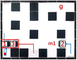
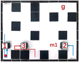
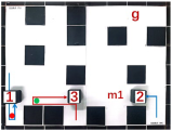
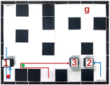
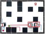
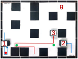
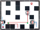
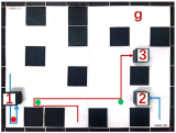
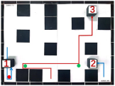
Multiple Robot Positions Corresponding to Each Time Step
0	1	2	3	4
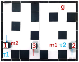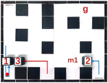5	6	7	8	9
10	11	12	13	14

details the travel trajectories of the sub-task robots and the task execution robot during the collaboration process. In the experiment, the two sub-task robots first move separately to their respective task starting points ${\tau }_1$ and ${\tau }_2$ to acquire and prepare to execute their corresponding tasks. Subsequently, they proceed to adjacent grid positions near their respective meeting points $m_1$ and $m_2$, where they stop moving and wait for the arrival of the task execution robot to perform task handover. According to the data in Table 3, the two sub-task robots successfully handed over their tasks to the task execution robot at time step 4 and time step 9. Ultimately, the task execution robot is responsible for delivering both sub-tasks to the designated task goal point $g$, thereby completing the collaborative task. This experimental process fully validates the Co-${\mathrm{D}\mathrm{P}\mathrm{S}\mathrm{I}\mathrm{P}\mathrm{P}}_{\mathrm{m}\mathrm{s}}$ algorithm’s effectiveness with multiple meeting points regarding path planning and coordinating robot collaboration.

7. Conclusions

Co-MAPF surpasses traditional MAPF in tackling tasks and significantly enhances system efficiency in most cases. In this paper, we innovatively propose a multi-robot path-planning algorithm to solve the problem of “many-to-one” collaborative robot tasks, which allows collaborative agents to perform task handovers at multiple meeting points. This advancement effectively mitigates the issue of excessively long redundant paths that occur during task handovers at a single meeting point. Furthermore, we incorporate an automatic switching strategy between multi-meeting-point and single-meeting-point solving modes to boost solution success rates. When the multi-meeting-point solving mode encounters difficulties, the algorithm seamlessly transitions to the single-meeting-point solving mode, ensuring a greater likelihood of successful solutions.

The simulation results unequivocally demonstrate the superiority of the proposed Cooperative Dynamic Priority Safe Interval Path Planning with multi-meeting-point and single-meeting-point solving mode switching (Co-${\mathrm{D}\mathrm{P}\mathrm{S}\mathrm{I}\mathrm{P}\mathrm{P}}_{\mathrm{m}\mathrm{s}}$) algorithm. Compared to the Co-CBS algorithm, Co-${\mathrm{D}\mathrm{P}\mathrm{S}\mathrm{I}\mathrm{P}\mathrm{P}}_{\mathrm{m}\mathrm{s}}$ achieves an average 39.20% increase in the solution success rate, a 9.45% reduction in total path length, and a 56.65% decrease in the solution time. Compared to Co-${\mathrm{D}\mathrm{P}\mathrm{S}\mathrm{I}\mathrm{P}\mathrm{P}}_{\mathrm{s}}$, the variant with a single meeting point, Co-${\mathrm{D}\mathrm{P}\mathrm{S}\mathrm{I}\mathrm{P}\mathrm{P}}_{\mathrm{m}\mathrm{s}}$, exhibits a 15.4% improvement in the solution success rate, a 12.03% reduction in the total path length, and a 14.23% decrease in the total path cost. These findings indicate that the Co-${\mathrm{D}\mathrm{P}\mathrm{S}\mathrm{I}\mathrm{P}\mathrm{P}}_{\mathrm{m}\mathrm{s}}$ algorithm significantly enhances solution success rates and shortens path lengths. Notably, as the number of agents within a specific range increases, the optimization effects on the total path length and cost become more pronounced, highlighting the scalability and efficiency of the proposed algorithm. Finally, the practicality and feasibility of the path planning solution devised by our algorithm are further validated through the actual execution results of CoCube agents.

In the future, we will focus on several core areas to deeply optimize algorithms, including enhancing algorithm execution efficiency, improving the quality of path planning solutions, achieving scientific and rational task allocation, and strengthening the collaborative working mechanism among multiple agents. Our goal is to realize more efficient and superior path-planning solutions.

References

- Stern, R.; Sturtevant, N.; Felner, A.; Koenig, S.; Ma, H.; Walker, T.T.; Li, J.; Atzmon, D.; Cohen, L.; Satish Kumar, T.K.; et al. Multi-agent pathfinding: Definitions, variants, and benchmarks. In Proceedings of the International Symposium on Combinatorial Search, Napa, CA, USA, 16–17 July 2019; Volume 10, pp. 151–158. [Google Scholar]
- Ren, Z.; Rathinam, S.; Choset, H. A conflict-based search framework for multiobjective multiagent path finding. IEEE Trans. Autom. Sci. Eng. 2022, 20, 1262–1274. [Google Scholar] [CrossRef]
- Ali, Z.A.; Yakovlev, K. Safe Interval Path Planning with Kinodynamic Constraints. In Proceedings of the AAAI Conference on Artificial Intelligence, Washington, DC, USA, 7–14 February 2023; Volume 37, pp. 12330–12337. [Google Scholar]
- Cohen, L.; Wagner, G.; Chan, D.; Choset, H.; Sturtevant, N.; Koenig, S.; Satish Kumar, T.K. Rapid randomized restarts for multi-agent path finding solvers. In Proceedings of the International Symposium on Combinatorial Search, Stockholm, Sweden, 14–15 July 2018; Volume 9, pp. 148–152. [Google Scholar]
- Lin, C.; Han, G.; Du, J.; Xu, T.; Lv, Z. Spatiotemporal congestion-aware path planning toward intelligent transportation systems in software-defined smart city IoT. Internet Things J. 2020, 7, 8012–8024. [Google Scholar] [CrossRef]
- Yu, C.; Jia-Qiang, E.; Hao, Z.; Yuan-Wang, D. Driving-Record-Based Distributed Path-Planning for Autonomous Vehicle. In Proceedings of the International Conference on Intelligent Transportation, Big Data and Smart City, Xi’an, China, 19–20 December 2015; pp. 320–323. [Google Scholar]
- Sun, N.; Shi, H.; Han, G.; Wang, B.; Shu, L. Dynamic path planning algorithms with load balancing based on data prediction for smart transportation systems. IEEE Access 2020, 8, 15907–15922. [Google Scholar] [CrossRef]
- Fu, X.; Li, C.; Hui, Y.; Hui, Y.; Yang, J. Space-Time Map Based Path Planning solution in Large-Scale Intelligent Warehouse System. In Proceedings of the International Conference on Intelligent Transportation Systems, Rhodes, Greece, 20–23 September 2020; pp. 1–6. [Google Scholar]
- Shi, Y.; Hu, B.; Huang, R. Task allocation and path planning of many robots with motion uncertainty in a warehouse environment. In Proceedings of the International Conference on Real-Time Computing and Robotics, Xining, China, 15–19 July 2021; pp. 776–781. [Google Scholar]
- Chen, X.; Li, Y.; Liu, L. A coordinated path planning algorithm for multi-robot in intelligent warehouse. In Proceedings of the International Conference on Robotics and Biomimetics, Dali, China, 6–8 December 2019; pp. 2945–2950. [Google Scholar]
- Wen, H.; Lin, Y.; Wu, J.B. Co-evolutionary optimization algorithm based on the future traffic environment for emergency rescue path planning. IEEE Access 2020, 8, 148125–148135. [Google Scholar] [CrossRef]
- Dresner, K.; Stone, P. A multiagent approach to autonomous handover point management. J. Artif. Intell. Res. 2008, 31, 591–656. [Google Scholar] [CrossRef]
- Le, C.; Pham, H.X.; La, H.M. A Multi-Robotic System for Environmental Cleaning. arXiv 2018, arXiv:1811.00690. [Google Scholar]
- Phillips, M.; Likhachev, M. Sipp: Safe interval path planning for dynamic environments. In Proceedings of the 2011 IEEE International Conference on Robotics and Automation, Shanghai, China, 9–13 May 2011; pp. 5628–5635. [Google Scholar]
- Silver, D. Cooperative pathfinding. In Proceedings of the AAAI Conference on Artificial Intelligence and Interactive Digital Entertainment, Marina Del Rey, CA, USA, 1–3 June 2005; Volume 1, pp. 117–122. [Google Scholar]
- Sharon, G.; Stern, R.; Felner, A.; Sturtevant, N.R. Conflict-based search for optimal multi-agent pathfinding. Artif. Intell. 2015, 219, 40–66. [Google Scholar] [CrossRef]
- Wagner, G.; Choset, H. M*: A complete multirobot path planning algorithm with performance bounds. In Proceedings of the International Conference on Intelligent Robots and Systems, San Francisco, CA, USA, 25–30 September 2011; pp. 3260–3267. [Google Scholar]
- Lan, X.; Lv, X.; Liu, W.; He, Y.; Zhang, X. Research on robot global path planning based on improved A-star ant colony algorithm. In Proceedings of the 2021 IEEE 5th Advanced Information Technology, Electronic and Automation Control Conference (IAEAC), Xi’an, China, 12–14 March 2021; Volume 5, pp. 613–617. [Google Scholar]
- Narayanan, V.; Phillips, M.; Likhachev, M. Anytime safe interval path planning for dynamic environments. In Proceedings of the 2012 IEEE/RSJ International Conference on Intelligent Robots and Systems, Algarve, Portugal, 7–12 October 2012; pp. 4708–4715. [Google Scholar]
- Yakovlev, K.; Andreychuk, A.; Stern, R. Revisiting bounded-suboptimal safe interval path planning. In Proceedings of the International Conference on Automated Planning and Scheduling, Nancy, France, 26–30 October 2020; Volume 30, pp. 300–304. [Google Scholar]
- Barer, M.; Sharon, G.; Stern, R.; Felner, A. Suboptimal variants of the conflict-based search algorithm for the multi-agent pathfinding problem. In Proceedings of the International Symposium on Combinatorial Search, Prague, Czech Republic, 15–17 August 2014; Volume 5, pp. 19–27. [Google Scholar]
- Boyarski, E.; Felner, A.; Stern, R.; Sharon, G.; Betzalel, O.; Tolpin, D.; Shimony, E. Icbs: The improved conflict-based search algorithm for multi-agent path finding. In Proceedings of the International Symposium on Combinatorial Search, Jerusalem, Israel, 11–13 June 2015; Volume 6, pp. 223–225. [Google Scholar]
- Li, J.; Ruml, W.; Koenig, S. EECBS: A bounded-suboptimal search for multi-agent path finding. In Proceedings of the AAAI Conference on Artificial Intelligence, New York, NY, USA, 2–9 February 2021; Volume 35, pp. 12353–12362. [Google Scholar]
- Ma, H.; Li, J.; Kumar, T.K.; Koenig, S. Lifelong multi-agent path finding for online pickup and delivery tasks. arXiv 2017, arXiv:1705.10868. [Google Scholar]
- Greshler, N.; Gordon, O.; Salzman, O.; Shimkin, N. Cooperative multi-agent path finding: Beyond path planning and collision avoidance. In Proceedings of the 2021 International Symposium on Multi-Robot and Multi-Agent Systems (MRS), Cambridge, UK, 4–5 November 2021; pp. 20–28. [Google Scholar]
- Sun, S.; Gu, C.; Wan, Q.; Huang, H.; Jia, X. CROTPN based collision-free and deadlock-free path planning of AGVs in logistic center. In Proceedings of the 2018 15th International Conference on Control, Automation, Robotics and Vision (ICARCV), Singapore, 18–21 November 2018; pp. 1685–1691. [Google Scholar]
- Salzman, O.; Stern, R. Research challenges and opportunities in multi-agent path finding and multi-agent pickup and delivery problems. In Proceedings of the 19th International Conference on Autonomous Agents and MultiAgent Systems, Auckland, New Zealand, 9–13 May 2020; pp. 1711–1715. [Google Scholar]
- Wang, N.; Yang, X.; Wang, T.; Xiao, J.; Zhang, M.; Wang, H.; Li, H. Collaborative path planning and task allocation for multiple agricultural machines. Comput. Electron. Agric. 2023, 213, 108218. [Google Scholar] [CrossRef]
- Wang, X.; Yang, L.; Huang, Z.; Ji, Z.; He, Y. Collaborative path planning for agricultural mobile robots: A review. In Proceedings of the International Conference on Autonomous Unmanned Systems, Beijing, China, 24–26 September 2021; pp. 2942–2952. [Google Scholar]
- Alshammrei, S.; Boubaker, S.; Kolsi, L. Improved Dijkstra algorithm for mobile robot path planning and obstacle avoidance. Comput. Mater. Contin. 2022, 72, 5939–5954. [Google Scholar] [CrossRef]
- Chen, Q.; Zhao, Q.; Zou, Z. Threat-oriented collaborative path planning of unmanned reconnaissance mission for the target group. Aerospace 2022, 9, 577. [Google Scholar] [CrossRef]
- Zhi, L.; Zuo, Y. Collaborative Path Planning of Multiple AUVs Based on Adaptive Multi-Population PSO. J. Mar. Sci. Eng. 2024, 12, 223. [Google Scholar] [CrossRef]
- Zhang, X.; Xia, S.; Li, X.; Zhang, T. Multi-objective particle swarm optimization with multi-mode collaboration based on reinforcement learning for path planning of unmanned air vehicles. Knowl. Based Syst. 2022, 250, 109075. [Google Scholar] [CrossRef]
- Atia MG, B.; El-Hussieny, H.; Salah, O. A supervisory-based collaborative obstacle-guided path refinement algorithm for path planning in wide terrains. IEEE Access 2020, 8, 214672–214684. [Google Scholar] [CrossRef]
- Grenouilleau, F.; Van Hoeve, W.J.; Hooker, J.N. A multi-label A* algorithm for multi-agent pathfinding. In Proceedings of the International Conference on Automated Planning and Scheduling, Berkeley, CA, USA, 11–15 July 2019; Volume 29, pp. 181–185. [Google Scholar]
- Atzmon, D.; Felner, A.; Li, J.; Shperberg, S.; Sturtevant, N.; Koenig, S. Conflict-tolerant and conflict-free multi-agent meeting. Artif. Intell. 2023, 322, 103950. [Google Scholar] [CrossRef]
- Motes, J.; Sandström, R.; Lee, H.; Thomas, S.; Amato, N.M. Multi-robot task and motion planning with sub-task dependencies. IEEE Robot. Autom. Lett. 2020, 5, 3338–3345. [Google Scholar] [CrossRef]
- Li, J.; Tinka, A.; Kiesel, S.; Durham, J.W.; Kumar, T.S.; Koenig, S. Lifelong multi-agent path finding in large-scale warehouses. In Proceedings of the AAAI Conference on Artificial Intelligence, New York, NY, USA, 2–9 February 2021; Volume 35, pp. 11272–11281. [Google Scholar]
- Teichteil-Koenigsbuch, F.; Poveda, G. Collaborative common path planning in large graphs. Aerosp. Lab 2020, 1–12. [Google Scholar] [CrossRef]
- Pan, Z.; Li, M. Path planning for collaborative robot under complex biomedical lab environment. In Proceedings of the 2022 7th International Conference on Control, Robotics and Cybernetics (CRC), Zhanjiang, China, 15–17 December 2022; pp. 17–22. [Google Scholar]
- Hegde, A.; Ghose, D. Multi-UAV collaborative transportation of payloads with obstacle avoidance. IEEE Control. Syst. Lett. 2021, 6, 926–931. [Google Scholar] [CrossRef]
- Ma, H.; Tovey, C.; Sharon, G.; Kumar, T.K.; Koenig, S. Multi-agent path finding with payload transfers and the package-exchange robot-routing problem. In Proceedings of the AAAI Conference on Artificial Intelligence, Phoenix, AZ, USA, 12–17 February 2016; Volume 30. [Google Scholar]