Abstract
The definition of multiple operational modes in a satellite is of vital importance for the adaptation of the satellite to the operational demands of the mission and environmental conditions. In this work, three optimization methods were implemented for the initial calibration of an attitude controller based on fuzzy logic with the purpose of performing an initial exploration of optimal regions of the design space: a multi-objective genetic algorithm (GAMULTIOBJ), a particle swarm optimization (PSO), and a multi-objective particle swarm optimization (MOPSO). The performance of the optimizers was compared in terms of energy cost, accuracy, computational cost, and convergence capabilities of each algorithm. The results show that the PSO algorithm demonstrated superior computational efficiency compared to the others. Concerning the exploration of optimum regions, all algorithms exhibited similar exploratory capabilities. PSO’s low computational cost allowed for thorough scanning of specific interest regions, making it ideal for detailed exploration, whereas MOPSO and GAMULTIOBJ provided more balanced performance with constrained Pareto front elements.
1. Introduction
The Attitude Determination and Control System (ACDS) of a satellite is a fundamental component, as it ensures the correct orientation with respect to a specific reference. The appropriate orientation of the satellite is not only essential for the nominal operation of the satellite but also during the so-called pointing maneuvers. In the first case, it may be necessary to maintain a specific orientation of the satellite relative to a certain reference throughout its orbit. For example, this is crucial for maintaining constant and optimal solar illumination conditions in sun-synchronous orbits or for keeping an optical sensor continuously pointed at a specific region of the earth’s surface in the case of geostationary orbits. However, it may also be necessary to orient the satellite in a different manner for a brief period through a pointing maneuver.
Therefore, the success of a space mission often depends on having the appropriate orientation of the satellite at a specific moment in time. Given that the energy stored in a satellite is limited and can affect its operational life, it is crucial to optimize the ADCS energy and computational efficiency to maximize the resources allocated to the payload and not constrain the functioning of other subsystems. This issue is particularly pronounced in the case of nanosatellites, as their small size limits the available energy, and most of them are deployed in low Earth orbits (LEO), characterized by periods of eclipse during which the solar panels are rendered inoperative (see [1,2] and references inside). Additionally, the satellites are subject to various space disturbances that influence their orbital dynamics. For this reason, a robust and stable control system is necessary to counteract external perturbations. In summary, the main characteristics that satellite attitude control systems must possess are energy efficiency, pointing accuracy, and robustness.
Currently, multiple control systems have been studied in the space domain (see [1] for a historical overview). There has been a notable increase in interest in recent decades in systems based on fuzzy logic [1,3]. The excellent results obtained in these studies confirm fuzzy logic controllers as an alternative to consider compared to classical controllers commonly used today, such as proportional, integral, derivative (PID) [1,3,4] or linear quadratic regulator (LQR) [2]. However, their practical application is still limited due to the difficulty of validating these algorithms in space missions or ground experiments and the high reliability requirements of space missions. This, in turn, leads to the slow adoption of new technologies in the space domain.
This work, however, does not focus on the design and comparison of different types of controllers as previous studies do. Instead, it aims to provide a specific type of controller with various operating points by using different heuristic optimization methods along with simulation software that emulates the space conditions to which the satellite will be subjected in orbit. The optimal operating points achieved will represent different combinations of energy cost and accumulated error maneuver; so, depending on the mission requirements, different operating points can be chosen. Clearly, the set of operating points provided by each algorithm will differ from the rest, but the purpose here is not to determine if one method is better than another but rather to explore their performances, capabilities, and limitations to establish when the use of a particular one would be appropriate.
In particular, the main points of interest to explore are, on one hand, to study which methods provide better optimal points on the Pareto fronts that optimize energy cost and accumulated error depending on the mission requirements. Regardless of the nature of the algorithm, in all cases, a Pareto front is constructed, which is essentially the collection of the operating points. The Pareto fronts give a comparative basis for the algorithms and also provide a flexible controller capable of changing its operational mode according to the required conditions at a given time. To achieve this, however, the operational conditions must be measured in real time, and part of the onboard computer’s memory must be reserved for storing the various controller operating points. In reality, this is not a problem because the new computers that are onboard space missions are already powerful enough to store and select the appropriate controller in each case [5,6]. On the other hand, the comparison focuses on studying the advantages and disadvantages of using multi-objective methods versus mono-objective methods, given that there is always a trade-off between several objectives in nanosatellite missions. Finally, a comparison in terms of computational efficiency is needed, as obtaining Pareto fronts is generally computationally costly.
Heuristic methods have been developed to address challenges such as non-linearity, multi-objectivity, and uncertainty. Their mechanisms, inspired by natural phenomena and incorporating randomness, make them suitable for solving complex global optimization problems or problems where the shape of the objective function is unknown. Although they do not guarantee the achievement of the global optimum, they provide a very good approximation of it. In recent decades, new heuristic algorithms have continued to be developed (see Table 1 in [7]), but the use of algorithms based on GA (genetic algorithm) and PSO (particle swarm optimization) remains prevalent when tackling multi-objective problems. GA is particularly well suited for applied engineering problems, where a trade-off between multiple conflicting objectives is the usual scenario [8]. Additionally, there are countless variants of each algorithm, and they have often been tested against each other to find the most suitable at solving a variety of problems (see [9,10,11,12,13] and references inside). An in-depth look at the historical development and applications of various PSO-based algorithms is provided in [14,15], and an extensive review of the state-of-the-art of variants and advancements of PSO algorithms can be found in [16]. An analogous study for the GA was conducted in [17].
In the present work, three different optimization methods—a multi-objective genetic algorithm and two algorithms derived from the original PSO—are implemented to achieve different operating points of the attitude control subsystem of the OPS-SAT satellites [18]. OPS-SAT are experimental satellites operated by the European Space Agency (ESA), which serve as powerful, reconfigurable flying laboratories for experiments. Currently, the first OPS-SAT has completed its operational life, and the next one, the OPS-SAT 2, will be launched soon. A comparative study of the performance of the optimization algorithms in terms of energy cost, pointing accuracy, computational cost, and convergence capabilities of each algorithm were conducted.
2. Materials and Methods
This section describes the OPS-SAT scenery, where the simulations were performed, the attitude controller, the optimization algorithms and the metrics used.
2.1. OPS-SAT Scenery
One of the main problems to verify operational reliability and certification is the lack of experimental opportunities in orbit. Most of the works are simulations, and the experimental data are usually obtained on ground with air-bearing test beds. A few years ago, ESA offered the researchers the opportunity to propose experiments to be carried out on-board the OPS-SAT laboratories. OPS-SAT are experimental satellites operated by the ESA, which serve as powerful, reconfigurable flying laboratories for experiments. The motivation behind its construction stems from the difficulty of conducting in-orbit control system tests, where the risk of losing a valuable satellite is high. Hence, the possibility of participating in missions such as the OPS-SAT platforms is a great opportunity to test new control algorithms in orbit. This is the reason why the simulation scenario used in this study was based on the conditions of the first OPS-SAT satellite.
OPS-SAT is a low-cost, secure satellite with high robustness. These qualities enable it to carry and test new control software with the confidence that the satellite can be recovered even if experimental applications push it to its operational limits, thus safeguarding the mission.
Meeting the dual requirements of high performance and safety while keeping costs low is a significant challenge. To address this, the OPS-SAT mission combines readily available subsystems commonly used in CubeSats with cutting-edge terrestrial microelectronics for the on-board computer. Additionally, the team leverages the extensive experience gained by the ESA in safely operating satellites over the past 40 years.
OPS-SAT also capitalizes on the latest research in mission operations for CubeSats. It employs the NanoSat MO Framework (NMF), which treats software deployment in space like simple apps on Android or iOS. Developed through ESA research and development, the NMF was first demonstrated in ESA’s OPS-SAT mission. It provides a way to upload and upgrade on-board apps, fully decoupling app features from the underlying hardware. The NMF offers straightforward integration through an API and tutorials, allowing app developers to focus on functionality without mastering the intricacies of spacecraft hardware. With the NMF, app developers can easily access key spacecraft peripherals such as GPS receivers, cameras, sensors, and telemetry parameters. Furthermore, the NMF facilitates app orchestration and operation, even from ground control [19].
The OPS-SAT spacecraft and its payloads are managed using the Satellite Experimental Processing Platform (SEPP). The SEPP offers comprehensive control over the spacecraft by providing high- and low-level interfaces to experimenters. If any unexpected behavior or potential risks arise, the currently active OPS-SAT onboard computer (OBC) takes over and interrupts the experiment to ensure the spacecraft’s safety. This innovative approach allows for testing and validating new techniques in mission control and onboard satellite systems while maintaining robust safety measures [20]. The OPS-SAT satellite was injected into a Sun-synchronous orbit (SSO) known as the 06–18 (“Dusk–Dawn”) orbit, characterized by maintaining a constant orientation of its orbital plane relative to the solar meridian. In a preliminary analysis, considering that generally the eccentricity and the major axis of the orbit are determined by other mission requirements, achieving heliosynchronicity is primarily determined by setting the inclination to match the secular precession of the nodal line with the angular velocity of the solar meridian. Additionally, since the local solar time at the subsatellite point depends solely on the latitude fixed by the inclination, Sun-synchronous orbits enable constant local solar time observations over specific regions of interest on the earth’s surface.
The geometry of the OPS-SAT satellite, as depicted in Figure 1, primarily consists of a prismatic body of three CubeSat units and two rectangular solar panels.
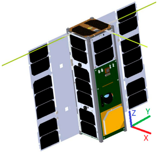
Figure 1.
OPS-SAT scheme. Courtesy of ESA and the OPS-SAT design team.
For special experiments that require a specific satellite pointing, the ADCS payload system can be used. The ADCS payload allows implementation of standard pointing modes like Earth Target Pointing or the implementation of custom pointing algorithms from within the SEPP [21]. It provides the experimenters with access to sensors and actuators as well as integrated attitude control functionality [18]. OPS-SAT is equipped with gyros, accelerometers, magnetometers, a Star Tracker, and six reaction wheels, with each body axis containing two aligned and all meeting identical technical specifications. Additionally, it features magnetorquers with different maximum dipole moments. The satellite’s body-frame system is centered on its center of mass, with its axes aligned parallel to those shown in Figure 1.
Attitude reference is chosen based on the operational requirements of the power and communication subsystems, linking the attitude reference system to the solar and nadir directions. The goal is to keep the face with the antenna aligned with the local vertical (nadir) to facilitate communications. Concurrently, maximizing illumination on the face with the main array of solar cells involves tracking Earth regions where sunrise or sunset angles are ideally zero. However, errors in injection and accumulated perturbations, which the satellite cannot correct due to lack of orbital trajectory adjustment capabilities, may lead to deviations from this nominal attitude.
Deviation from this nominal attitude may significantly affect the satellite’s exposed surface, influencing the magnitude of aerodynamic disturbances and solar radiation pressure. It is crucial to consider upper limits for these disturbances to ensure sufficient actuator capacity during the most unfavorable scenarios.
Currently, the first OPS-SAT has completed its operational life. The app to test the controller was uplinked and correctly installed in the first OPS-SAT, and it was executed several times. Therefore, it complied with the framework structure, and all the described functionalities were successfully tested. Nevertheless, due to a malfunction of the I2C bus, the connection to the ADCS was lost after a few seconds, freezing the subsystem telemetry and preventing the subsystem from accepting commands. After several troubleshooting and workarounds were implemented, the OPS-SAT Flight Control Team acknowledged there was nothing else that could be done from ground to improve the situation. For this reason, there are no experimental results from the in-orbit experiment. We are confident in being able to re-run it successfully in the upcoming OPS-SAT 2 mission.
2.2. Fuzzy Controller
Figure 2 shows the typical scheme of an attitude control loop, in which some blocks have been bypassed, as the main objective is the analysis of the controller block (see [1] for more detail). The plant would be the OPS-SAT satellite.
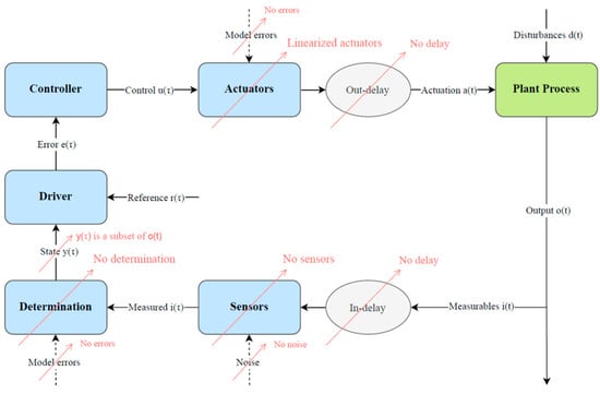
Figure 2.
Flowchart of all simulator functions involved in the simulation.
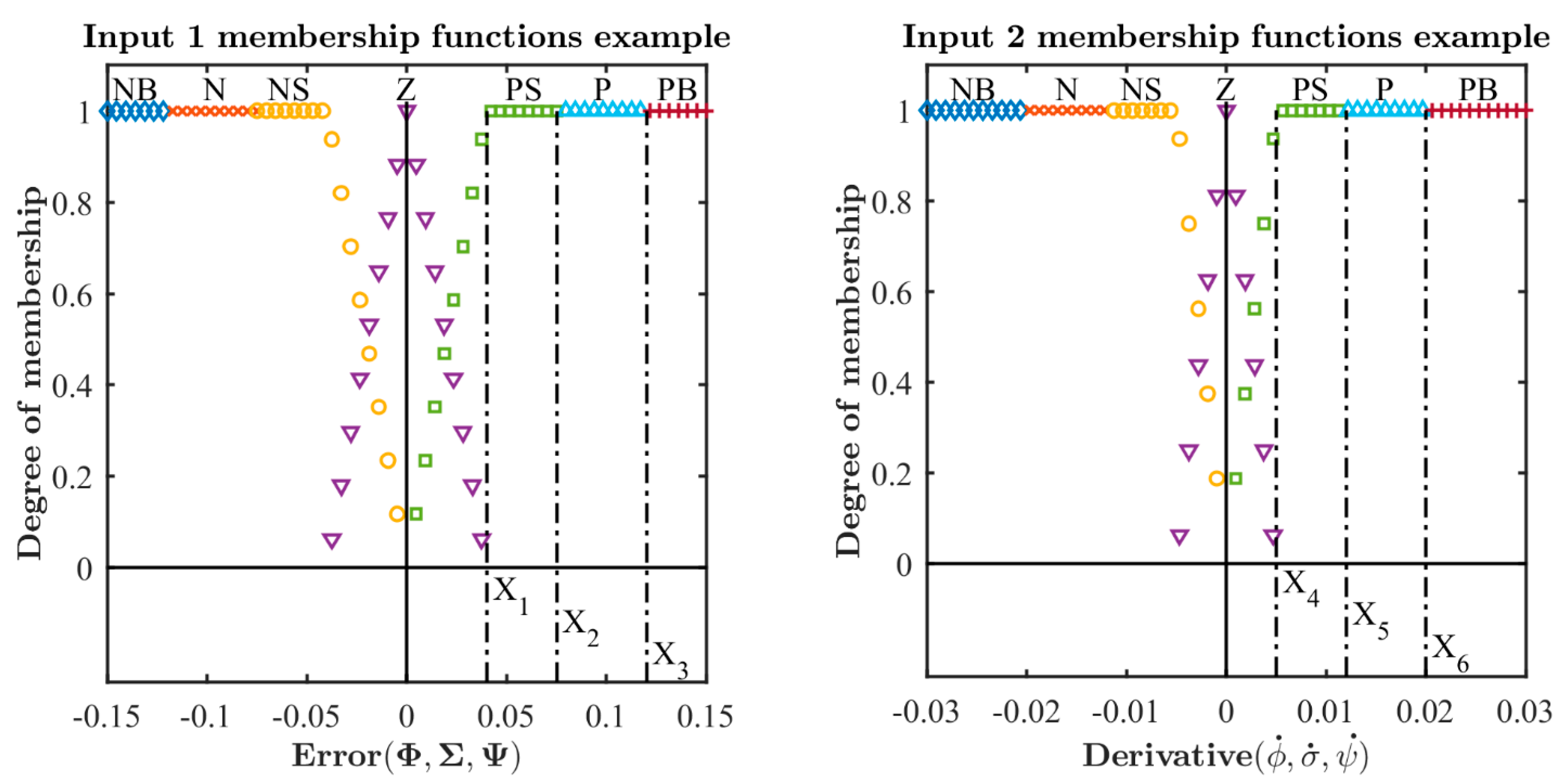
For the fuzzy controller, Figure 3 shows the input membership function shapes and the parameters needed to describe them (see [1] for more detail). The input variables are the attitude error and the angular velocity per axis. Six parameters are needed to fully describe the shape of the two input membership functions per axis: X = [x1 x2 x3 x4 x5 x6]. There are three controllers, with one per axis. Although the type of the membership functions is the same for the three axes, the X values are different, so a total of eighteen parameter values are needed to fully calibrate the system. These are the parameters that will be modified along the optimizations.
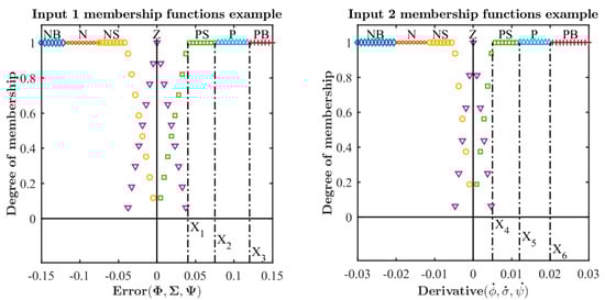
Figure 3.
Input membership functions with their six tuning parameters per axis, x1,…,x6. The domain values where they are null have not been represented for clarity.
The Takagi–Sugeno defuzzification method [22] was used for the fuzzy controllers in the three axes. As a result, there are no real membership functions associated with the values of the output linguistic variables but rather a list of discrete values representing the fraction of the maximum actuation that is needed.
2.3. Optimization Algorithms
In this work, three optimization algorithms were used to minimize two objectives: the accumulated pointing error and the energy cost of the controller during a maneuver, defined as follows:
The details of the definition of both objectives can be found in [1].
The optimizations provide different sets of the eighteen tuning parameters so that the main controller can pick the set to be used depending on the operational mode and its associated energy cost–accuracy directive. Due to the high number of tuning parameters, the controller optimization is split into three different optimizations, with one per axis.
Next, a brief description of the optimization algorithms used in this work is given: a multi-objective genetic algorithm modified (GAMULTIOBJ), a particle swarm optimization modified (PSO), and multi-objective particle swarm optimization (MOPSO).
2.3.1. Genetic Algorithms Modified
Genetic algorithms work on a coding of the set of design variables and do not require information about the gradient value (not even that it exists) or other auxiliary knowledge; it is sufficient to have the value of the objective function, making them algorithms that require little information about the problem. Additionally, they are very robust algorithms that are easy to understand, configure, and implement, and they work well in continuous, discrete, or mixed-optimization problems.
However, handling constraints in this method can be cumbersome. Moreover, despite finding multiple local optima that are far apart in the definition space, there is no knowledge of what the true global optimum is. In fact, in many problems, these algorithms converge to local minima or arbitrary points before reaching the global optimum, meaning that the algorithm does not manage to sacrifice “short-term fitness” to acquire “longer-term fitness”. Furthermore, they do not present clear termination criteria, as the best solution is only determined in comparison with other solutions, and their convergence is closely tied to their tuning parameters. Another issue with these algorithms is their poor scaling with complexity, understood as the number of degrees of freedom (or number of design variables). Despite all this, the main issue with these algorithms is the evaluation of the objective function in complex problems, as the computational cost of such an evaluation can be excessive. (This occurs in the final calibration of the controllers, as each evaluation of the objective function consists of running a simulation.) A solution is to take advantage of the good scalability of genetic algorithms with parallel computing since the evaluation of one individual is independent of the rest.
MATLAB R2023b© offers the capability to solve multi-objective optimization problems using genetic algorithms through its GAMULTIOBJ, which implements an elitist and controlled genetic algorithm that is a variant of the non-dominated sorting genetic algorithm (NSGA-II). The latter, encompassed within evolutionary multi-objective optimization (EMO), has three main characteristics: It employs an elitist principle that favors individuals with better objective function values, uses a specific mechanism to preserve diversity, and emphasizes dominant solutions.
The choice of the parameters is crucial, as the correct functioning of the algorithm and, consequently, the achievement of an acceptable solution depend on it.
Several modifications were implemented in the MATLAB© code (see [1] for more detail):
- (i)
- The first is related to the calculation of spread. This calculation was proposed in [23], but it was incorrectly implemented in the MATLAB© code. It was thus corrected.
- (ii)
- The second aspect concerns the way in which the spread change is calculated, represented by the variable “spreadChange”, which is involved in the stopping criterion. In the definition of the provided stopping criterion, abstract terms like “geometric mean of the relative change” were used, which needed clarification. Therefore, the original method of calculating this relative change was replaced by a mean that involves the differences in the spread value between one iteration and the immediately preceding iteration over a window of iterations. These changes were made in the file “gamultiobjConverged”.
- (iii)
- The third modification was made to the “stepgamultiobj.m” file, where the tolerance for finding duplicates in the population was reduced from 10−12 to 10−4, as the former was deemed excessive.
- (iv)
- The final modification is related to the function “DistanceMeasureFcn”. The “distancecrowding” function is the default for calculating distance; however, in the present work, this function was replaced by “distancecrowdingCustom”. Generally, the latter normalizes the objective values before computing the distances, which are calculated by summing the contributions from all dimensions in the objective space. This calculation involves distinguishing between distances at the extremes, which do not have two neighbors and therefore only consider the nearest neighbor, and the distances of the remaining points, calculated as half the difference for each objective between the distances to the immediately preceding and following neighbors. For the previous function, these distances were not divided by two, and the normalization of the values was not intuitive. Finally, the resulting “distancecrowding” vector is divided by the number of objectives (a step also omitted in the original function), and its extreme values are assigned an infinite distance, which was discarded in the subsequent calculation of the spread.
2.3.2. Particle Swarm Optimization Modified
In [24], an extensive identification of the main types of applications in which PSO has been successfully implemented was developed. More recently, an analysis of studies about PSO was carried out in [25]. Although this algorithm is classified within single-objective optimization, it can be applied to multi-objective optimization problems through the so-called utility function, a scalar function that allows converting the first type of problem into the second [26]. In this way, instead of optimizing a vector function, a scalar function combining (linearly or not) both objectives (energy cost and pointing error) can be optimized. In this study, for simplicity, the utility function was limited to a weighted sum of each objective.
Based on the references [26,27], the many advantages of PSO make it an alternative to be considered for solving global optimization problems. The first advantage of these algorithms, as with any other heuristic, is that they do not employ derivatives. Furthermore, the method stands out for its conceptual simplicity and ease of implementation, presenting lower sensitivity to the nature of the objective function compared to classical optimization methods or other heuristic techniques. The algorithm also has a reduced number of parameters, whose impact on the solutions is notably less sensitive than with other heuristic algorithms. Finally, PSO allows generating high-quality solutions with shorter computation time and more stable convergence characteristics than other stochastic methods, granting it notable efficiency and the ability to find the global optimum. Additionally, this algorithm is extensible to parallel computing.
However, PSO also presents a series of disadvantages. The biggest one, which it shares with other heuristic optimization techniques, is its lack of a solid mathematical foundation that allows for future analysis in the development of relevant theories [26]. Similarly, despite the algorithm’s impact on solutions being less negative than in other heuristic approaches, the method still has issues with dependence on initial values and parameters as well as the search for its ideal design parameters. The versatility of the algorithm to be applied to a wide variety of optimization problems without using the gradient of the problem to be optimized also comes with a cost [28], as PSO does not always work well and may require manual adjustment of its parameters by the user for proper operation. Finally, it should be noted that the speed of the algorithm may lead to premature convergence to local minima, especially in high-dimensional problems, where its performance deteriorates.
The algorithm that MATLAB© uses for PSO is the base algorithm described in [29], including certain modifications suggested in [28,30]. Compared to the original PSO algorithm introduced in [29], this algorithm introduces two main innovations. The first is that it is a variant of the “local best” PSO, where each particle is assigned a random subset of N additional particles with which it exchanges information. The second innovation is the inclusion of adaptive parameters, meaning parameters that modify their value throughout the algorithm. The use of adaptation mechanisms for the automatic control of certain variables allows for more effective search and better performance against local optima compared to the original algorithm, without excessively increasing implementation complexity. In this case, the adaptive parameters are reduced to two: the inertia weight and the neighborhood size, and both changes are based on the descriptions provided in [31,32]. The selection of PSO parameters and their impact on optimization performance has been the subject of extensive research [33,34,35,36,37].
Several modifications have been introduced in the MATLAB© code:
- (i)
- One of them is tied to the calculation of the algorithm’s convergence, as it is advisable to have well-defined and analogous stopping criteria to facilitate future comparisons between algorithms. For this same reason, the final stopping criterion was changed. Originally, the algorithm’s stopping criterion was encompassed in the “Improvement-Based Criteria” category [38] by accounting for any improvement in each iteration. The final stopping criterion proposed here is also of the “Improvement-Based Criteria” type. However, instead of monitoring the best objective function value in each iteration, a certain fraction of the best objective function values in each iteration is controlled, and a calculation like the spread change is performed. It is important to note that the best objective function values in each iteration consider, for all particles, the best position each has reached considering the current and all previous iterations and not only the particles that occupy the best positions in each iteration. To implement this change, an additional optional parameter called “ParetoFraction” was introduced into the algorithm, which establishes the fraction of individuals from the total population that will participate in the stopping criterion. For example, for a swarm of 100 particles and a ParetoFraction = 0.25, information about 25 particles and their best objective function values are collected for the stopping criterion calculation. Thus, the generated window is a matrix with as many columns as “MaxStallIterations” + 26 and as many rows as ParetoFraction x SwarmSize. In this way, once the first columns are sorted from the oldest to the most recent iteration and the rows from the best to the “worst” value, the relative change is computed as follows:
funChange = mean(mean(abs(bestFvalsWindow(:, 2:end)-bestFvalsWindow(:, 1:end-1))))
- (ii)
- Two optimization methods belonging to two different types are compared: single-objective optimization (PSO) and multi-objective optimization (GA). To facilitate the comparison, this study chose to construct the set of non-dominated points from all the positions attained by each particle in the swarm. For this purpose, the functions “outputFcnPSO” and “rateFcnOptimOPSSAT_PSO” were modified to store relevant information from the algorithm throughout all its iterations, such as the positions of the particles in each iteration, their associated utility function value, and the value of each objective of the original multi-objective problem. Dominance calculation implemented using this information from each iteration allowed us to build the Pareto front incrementally. Thus, a preliminary Pareto front was constructed with the initialization information. Then, the positions of the particles in the first iteration were added to the previous Pareto front, and the new set of non-dominated particles was recalculated. This process was repeated until all iterations were processed. It is important to realize that the calculation of dominance is performed based on the value of certain variables of the algorithm that are stored during each iteration. Therefore, all the necessary information will only be available once the algorithm stops. Thus, the dominance calculation is not part of the optimization itself but rather part of the post-processing of data.
2.3.3. Multi-objective Particle Swarm Optimization
The algorithm used is based on the multi-objective particle swarm optimization (MOPSO) variant proposed in [39]. This variant introduces a secondary population for elitism, aiming to maintain diversity and track non-dominated solutions throughout iterations. Unlike single-objective approaches, MOPSO handles multiple objectives by storing non-dominated vectors in an external repository, emphasizing leadership rather than simply constructing a Pareto front. This methodology enhances algorithm performance but requires careful management of diversity to avoid stagnation.
There are two distinct implementations of the MOPSO algorithm currently available:
- (i)
- Implementation by Víctor Martínez-Cagigal: This implementation is a vectorized version of the particle swarm, meaning it evaluates the objective function simultaneously for all particles. It requires the objective function to handle evaluation for each particle concurrently, which makes it impractical in cases where the objective function involves a prior simulation for each individual particle.
- (ii)
- Implementation by Mostapha Kalami Heris and Yarpiz: This implementation shares key characteristics with MOPSO, focusing on managing design variables within specified boundaries. It does not incorporate the strict handling of constraints present in the original MOPSO formulation, nor does it include innovations from [40]. One notable feature is the progressive damping of the inertia weight, emphasizing global exploration initially and gradually shifting towards local exploitation with each iteration.
Given these considerations, the implementation by Mostapha Kalami Heris and Yarpiz was chosen as the third optimization method in this study. However, it required adaptation within the simulation context due to its current limitations and design choices.
Next, the modifications made are described:
- (i)
- To adapt it to a simulation framework, the original script containing the MOPSO algorithm was transformed into a function that accepts all problem-specific data as input arguments. This function outputs the same data as the GAMULTIOBJ function: the Pareto front in the design and target space, the reason for termination, and a structured output containing relevant information (such as the final population with their objectives, iterations, evaluations, and metrics of the Pareto front like spread or average distance). Additionally, a history was added to track the values of certain variables throughout the entire optimization process. This adaptation ensures that the MOPSO algorithm aligns with the requirements and constraints of the specific simulation environment or problem being addressed.
- (ii)
- Another change made was the incorporation of two stopping criteria. Originally, the algorithm was designed to run for a predefined number of iterations. On the one hand, the calculation functions for spread and “distancecrowdingCustom” from the GA were adapted to implement the exact stopping criteria used in the multi-objective genetic algorithm. On the other hand, the algorithm stops when an optimization time is exceeded.
- (iii)
- The last change made to the algorithm was the replacement of the dominance calculation function with a vectorized and computationally more efficient version proposed by Víctor Martínez-Cagigal. Since this calculation represents a significant portion of the computational cost of the algorithm, this modification led to considerable improvements in computational time.
While this optimization may not be critical for calibration problems in control systems, since its optimization times are negligible compared to those of simulation, it provides an algorithm with less computational cost.
2.4. Metrics
The comparison between algorithms evaluates their performance both qualitatively and quantitatively. Quantitative evaluation relies on specific metrics calculated either from a single Pareto front or through direct comparisons between them. The metrics considered include algorithm effort (AE) and the ratio of non-dominated individuals (RNDI), which provide insights into optimization efficiency and the quality of solutions obtained by each algorithm. The AE [41] is defined as the ratio between the optimization time and the total number of objective function evaluations during that period:
In this study, since the number of evaluations is consistent across all algorithms, the AE metric serves as an indicator of how long each algorithm takes to complete a fixed number of iterations. A lower AE indicates faster performance. This metric is closely linked to optimization time, which measures the duration from algorithm invocation to output generation. Additionally, the RNDI metric simply calculates the proportion of non-dominated individuals (Pareto front members) within a population, providing insights into the quality of solutions produced by each algorithm:
So, a value of RNDI = 1 means that all elements of a population are non-dominated. Having a greater number of candidate solutions in a Pareto front after a certain number of iterations is desirable, which translates into high RNDI values.
Finally, concluding the section on metrics, four typical metrics of the multi-objective genetic algorithm were also included. The first two metrics are the average Pareto distance (APD) (which is the average of the crowding distance without considering the ends of the Pareto front, whose distance is by definition infinite); and the sum difference (SD), which represents the Euclidean norm of the difference between each point’s distance (crowding distance) and the average distance of the Pareto front. While the first metric provides the average distance value of a set of non-dominated points, the second provides information about how similar or different the distances of each point are relative to the average distance of the set, giving an idea of the uniformity of the set. In both cases, the term “distance” refers to the same concept: the distance from a point on the Pareto front to the semi-sum of distances to the nearest two points divided by the total number of dimensions, as mentioned earlier, without considering the extremes.
The other two metrics employed correspond to the so-called extreme Pareto distance (EPD) for the last iteration, which measures the movement of the extremes of the Pareto front relative to their position in the previous iteration, and the well-known spread. It is worth noting that spread measures the stability of the front rather than its uniformity, as it incorporates both the concept of uniformity and the movement of the front.
3. Results
Having studied the different algorithms whose results are herein compared and having examined the changes implemented in each of them, we proceeded with the optimization of the problems and the analysis of the results provided by each algorithm. Before starting the optimizations, a brief description of the calibration maneuver used is given.
3.1. Calibration Maneuver
The calibration maneuver selected is based on the typical maneuvers that a CubeSat needs to perform in an LEO. In such orbits, the satellite’s visibility from ground control centers is limited to a window of up to 15–30 min, depending on the orbit size and the distance from the subsatellite point to the ground station (greater time if this distance is zero and if the satellite’s trace passes over the station). During this time window, it is common to perform step maneuvers to quickly reorient the satellite to facilitate communication. Additionally, these maneuvers are frequent for orienting satellite instruments such as cameras and sensors.
The proposed experimentation for OPS-SAT involved performing maneuvers with increasing amplitude, starting with 5-degree turns and progressing to 20-degree turns. In the final experiments, the aim was to explore the operational limits of the controller with turns exceeding 30 degrees in amplitude. For these reasons, a 10-degree step was selected to characterize the calibration maneuver for OPS-SAT, which is divided into the following phases:
- -
- Initial phase: The angular error is approximately zero as the body axes align with the target axes. Its duration is 10 s and serves to evaluate initial stability metrics, assessing the controller’s ability to maintain the commanded attitude with an error signal below the established limit.
- -
- Step phase: A new attitude is commanded that deviates 10 degrees from the body axis being calibrated. The controller must act accordingly to achieve the target attitude within a variable time depending on the dynamics of the axis being calibrated;
- -
- Final phase: The target attitude is maintained for another 10 s and serves to evaluate residual stability metrics, assessing the controller’s ability to maintain an approximately zero angular error after the step phase.
The step phase allows for the evaluation of variables related to controller performance: the pointing error signal and the energy cost associated with the control law. Thus, the objective function adjusts the controller based on its calibration parameters, simulates the calibration maneuver, and evaluates the controller’s performance based on the accumulated error and the maneuver’s cost.
3.2. Optimization Results
In this section, the calibration of the fuzzy controller in the OPS-SAT simulation scenario is described. To achieve this, fifteen optimizations per algorithm were performed along a single axis, with results applicable to other axes. The calibrations aimed to maximize each algorithm’s capability in exploring optimal regions of the design space through a moderate number of predefined iterations (10), without concern for termination criteria related to search stability. Additionally, the initial populations used were randomly generated and always included a pair of manually selected members: one point with the lower error and another point with the lower cost, obtained similarly to [1].
When comparing algorithms performance, it is important to consider the different orders of magnitude in variable mutation between MOPSO and GAMULTIOBJ. In MOPSO, mutation initially spans the design space order and eventually reduces to order 0, while in GAMULTIOBJ, it varies based on the spread between 1 and 0. On the other hand, PSO does not involve mutation but utilizes adaptive inertia to balance global and local search. It is also noteworthy that this optimization problem includes constraints on design variables. Given that the PSO and MOPSO versions proposed here do not implement constraint handling, the objective function is penalized by returning a value of (1,1) when these constraints are violated.
The statistical parameters associated with the metrics obtained for each algorithm can be seen in Table 1.

Table 1.
Results for the metrics.
The PSO emerges as the fastest algorithm, demonstrating its high computational efficiency. The MOPSO shows competitive values, while the GAMULTIOBJ is relegated to the third position in terms of computational cost.
The mean and standard deviation of the number of elements obtained in the Pareto fronts with each algorithm are very similar. Noteworthy is the PSO’s capacity to generate more dominant individuals than the other two algorithms. (The minimum value of RNDI obtained was considerably higher than in the other cases.)
When exploring the design space, it is desirable for the Pareto front obtained to have the highest possible mean distances, and the MOPSO excels in this aspect. However, the GAMULTIOBJ shows the least deviation in terms of this factor.
The EPD metric will be important in subsequent optimizations aimed at refining the initial approximation obtained with these optimizations. Here, it is sufficient to know that the extremes of the fronts obtained with GAMULTIOBJ are those that show the least average and standard deviation in their movement for the calibrations performed.
Similarly to the EPD metric, the SD and spread metrics are more relevant in future optimizations that will aim to exploit the search in the optimal regions found. For the calibrations performed here, it was found that the Pareto fronts obtained with MOPSO exhibit the highest uniformity in their distances and the best spread values.
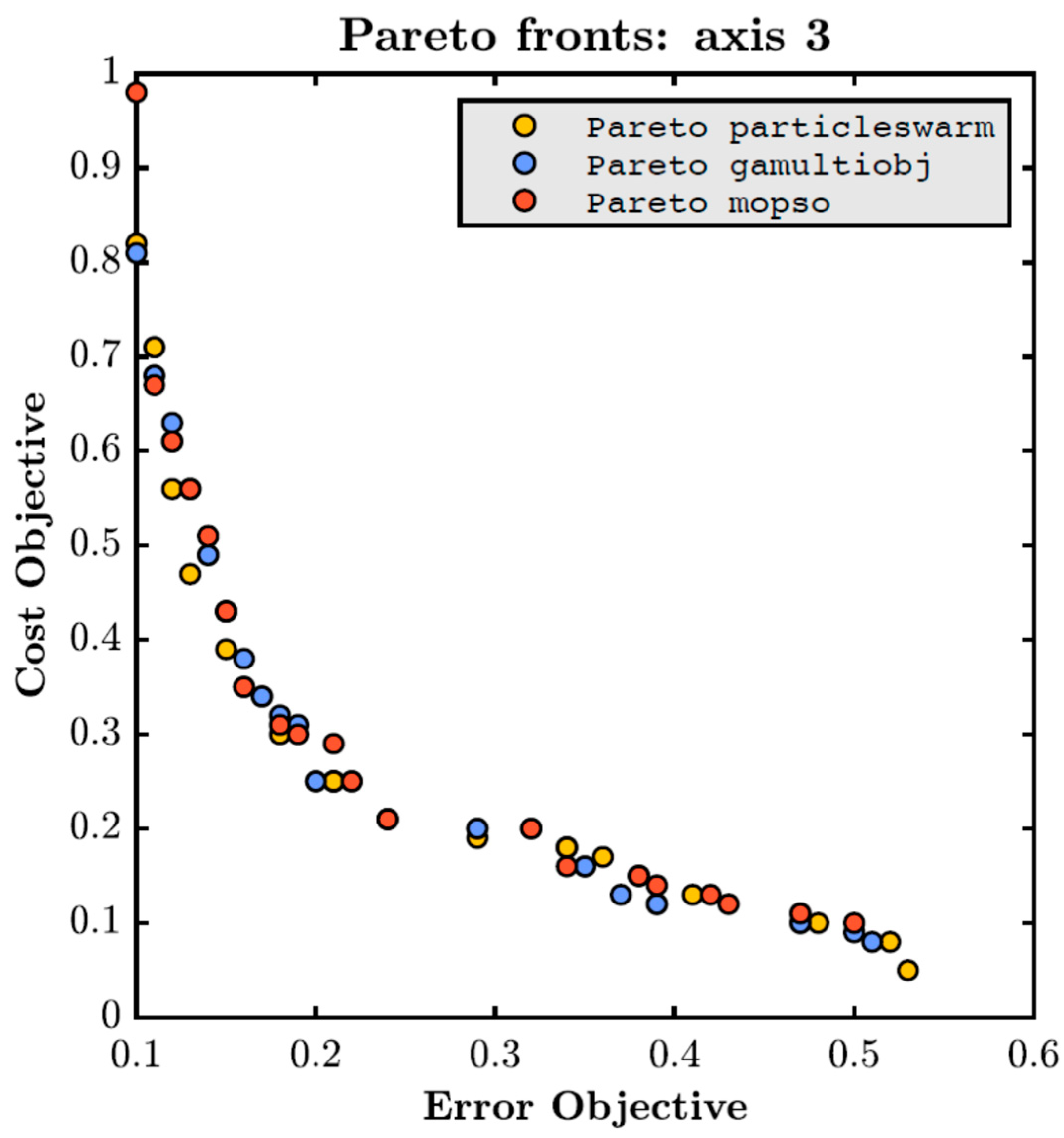
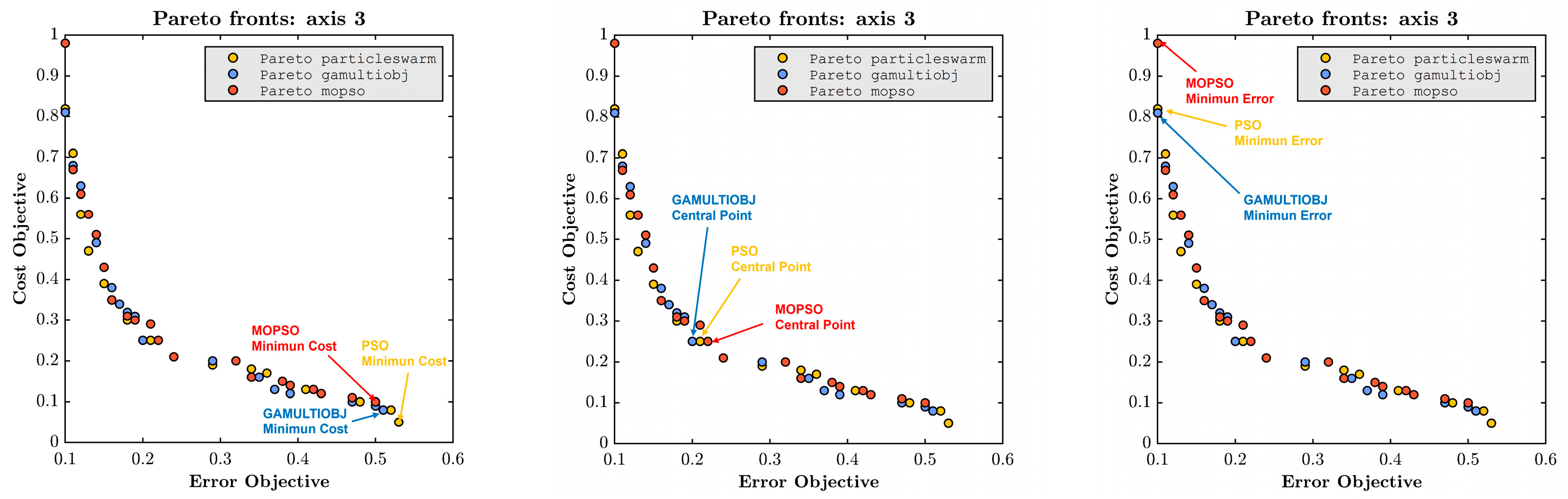
Finally, the set of non-dominated points was obtained based on the 15 Pareto fronts produced by each algorithm, thus deriving a “definitive” Pareto front. From the definitive Pareto front achieved with each algorithm, three characteristic points were calculated: the point of minimum error, the point of minimum cost, and the central point, which is the farthest from all extremes and is defined in [1]. The maneuver was also simulated for the design variable configurations associated with these points, obtaining the error signal and control actuation for each case. In Figure 4, a comparative graph between the different Pareto fronts provided by each algorithm for the yaw axis can be observed. As can be seen, the achieved results are generally similar. Figure 5 shows the three characteristic points: minimum error, minimum cost, and the central one of each optimizer in the Pareto front. Note that PSO and GAMULTIOBJ can find a minimum error design point like MOPSO, consuming 20% less energy. On the other hand, PSO found the lowest cost point but at the expense of having a higher error.
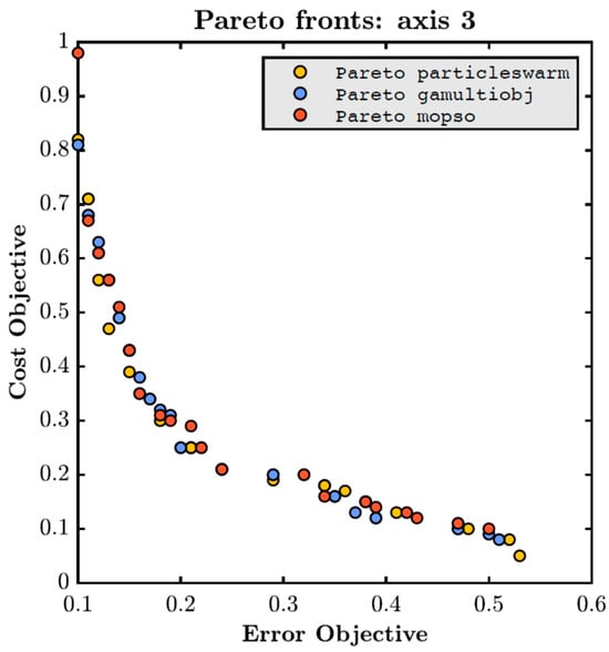
Figure 4.
Comparison of the three definitive Pareto fronts achieved with each algorithm for the yaw axis.
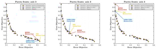
Figure 5.
Pareto fronts indicating central point, minimum cost, and minimum error for each optimizer.
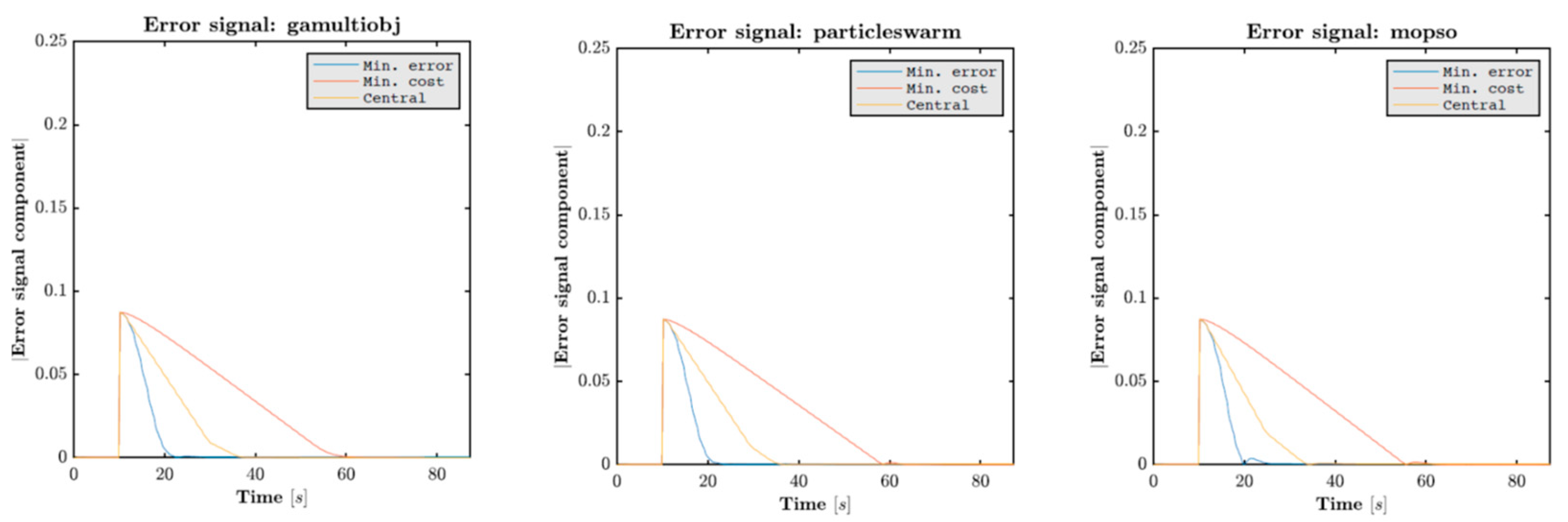
Figure 6 and Figure 7 show the specific results of each algorithm separately: the error signals and costs associated with their characteristic points. In all cases, the behavior of the error signal for the points of interest is the same, as it is maximal once the new target attitude is imposed and progressively decays depending on the chosen controller’s operating point. For the minimum error point, the signal decay is the fastest, while for the maximum error point (or minimum cost), the decay is the slowest. The rest of the optimal operating points obtained present error signals that fall within these extreme behaviors. Note that the MOPSO error profile shows an oscillation for the minimum error point around 20 s. This explains the higher energy cost of that point observed on the Pareto front.
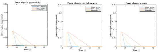
Figure 6.
Error signal associated with the characteristic points of the Pareto front: central point, minimum cost, and minimum error.
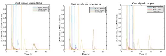
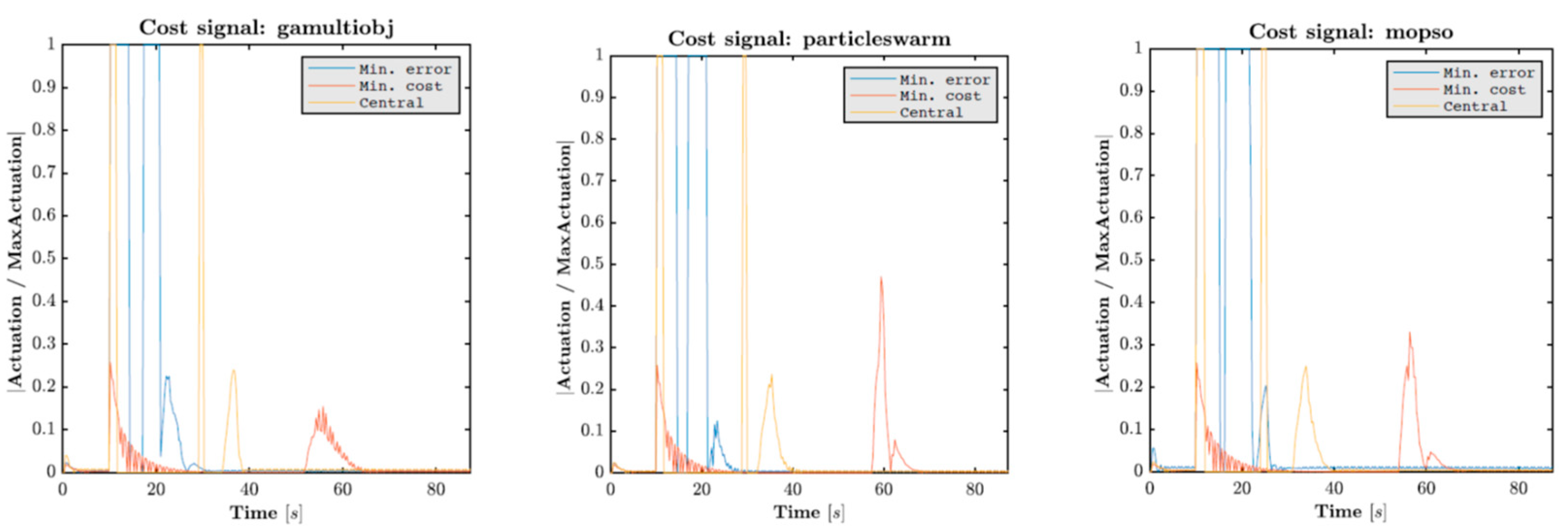
Figure 7.
Actuation associated with the characteristic points of the Pareto front: central point, minimum cost, and minimum error.
On the other hand, the actuation profile obtained with the fuzzy controller is based on impulses whose peaks occur when deviations from the commanded attitude occur. In the actuation profiles associated with the minimum error and central points in Figure 7, a total of three main impulses can be observed: an initial acceleration impulse followed by a zone of null actuation after reaching the desired angular velocity, a deceleration im-pulse to stop the system, and a modulation impulse to stabilize the final part. Regarding the actuation profile for the minimum cost point, only two main impulses were observed: an initial acceleration and a final deceleration modulation. All of them also presented an initial impulse that represents the stabilization of the controller around the state of null initial conditions.
4. Discussion
The definition of multiple operational modes in a satellite is of vital importance for adapting the satellite to the operational demands of the mission and the environmental conditions. In this work, three optimization methods were adapted and utilized for the initial calibration of a fuzzy controller, with the aim of conducting an initial exploration of optimal regions in the design space. The results achieved with PSO were promising in terms of computational cost, completing all optimizations in significantly less time compared to the other algorithms. MOPSO also showed considerable improvement in this aspect compared to GAMULTIOBJ. Despite most of the optimization time being spent on the simulation to evaluate each design variable, using a more computationally efficient algorithm resulted in optimization times of around 12 min for GAMULTIOBJ in the worst cases and only 8 and 5 min for MOPSO and PSO, respectively.
Moreover, the differences in optimization time do not diminish the exploratory capacity of each algorithm to find optimal regions in the design space, as this is very similar in all cases. In fact, considering the non-dominated points from the set of Pareto fronts obtained over a batch of 15 optimizations, the results achieved were practically identical.
Furthermore, the analysis of typical test functions with each algorithm allowed observation of the convergence capabilities of each algorithm as well as certain peculiarities in all of them. The Pareto front obtained with PSO can lead to a high concentration of non-dominated points that fit very well to the solution in one zone but differ significantly in the rest of the objective space. Additionally, the number of non-dominated elements obtained with this algorithm has no upper limit, allowing for highly populated Pareto fronts in some cases. Given the dependency on the weight used in the utility function, it is evident that PSO is an ideal algorithm for thoroughly scanning specific regions of interest (such as the extreme zones of the front). Since its computational cost is minimal, the algorithm also offers the possibility of superimposing the results of various optimizations, each exploring a specific region.
On the other hand, the Pareto fronts provided by GAMULTIOBJ and MOPSO present a maximum number of elements limited by certain parameters, and thus, their respective metrics related to distance will be a consequence of this fact.
5. Conclusions
Defining multiple operational modes in a satellite is crucial for adapting to mission demands and environmental conditions. In this study, three optimization methods were employed for the initial calibration of a fuzzy controller, aiming to explore optimal regions in the design space. The PSO algorithm demonstrated promising results regarding computational efficiency, completing optimizations significantly faster than the MOPSO and GAMULTIOBJ algorithms.
Despite the differences in optimization time, the exploratory capability of each algorithm in identifying optimal regions was comparable. Overall, PSO proved to be an ideal algorithm for efficiently exploring specific zones within the design space, while MOPSO and GAMULTIOBJ offered balanced performance with constrained element counts in their Pareto fronts.
Future studies will involve implementing constraints for the PSO and MOPSO algorithms. It is anticipated that the role of constraints in secondary optimizations, which refine the initial search, will become significant, making the use of penalty methods less suitable. Therefore, a study on the consideration of constraints in the calibration of fuzzy controllers is recommended. Additionally, it would be interesting to apply the proposed algorithms to the complete calibration of other types of controllers that do not involve constraints, such as PID controllers. It would also be very interesting to implement other optimization algorithms with the integration of predatory search strategy (PSS) and swarm intelligence technique, called PSS-PSO [15], which achieves a better performance compared with other PSO algorithms.
Concerning the controller design, future works could involve the improvement of the fuzzy controller by the design of a fuzzy neuron controller incorporating the dynamic pole concept (see [42]), which would provide a simpler controller that would facilitate optimizations.
For the upcoming OPS-SAT 2 mission, where several controllers will be tested and compared, the optimal regions of the design space will be obtained using either a MOPSO or a GAMULTIOBJ, and the regions of minimum cost, minimum error, and center will be refined by using a PSO. Additionally, the possibility of implementing a speed-constrained multi-objective PSO (SMPSO) algorithm (evolution of the MOPSO algorithm) could be considered.
Author Contributions
R.A., methodology, software, validation, and data curation, Visualization; K.S.O., conceptualization, methodology, and software; Á.B., conceptualization, software, and validation; J.J.F., supervision and project administration; V.L., conceptualization, writing—original draft, supervision, and project administration. All authors have read and agreed to the published version of the manuscript.
Funding
This research received no external funding.
Data Availability Statement
Data are contained within the article.
Acknowledgments
We would like to thank the E-USOC, the research group Aerospace Sciences and Operations of the Universidad Politécnica de Madrid (UPM).
Conflicts of Interest
The authors declare no conflicts of interest.
References
- Bello, Á.; del Castañedo, Á.; Olfe, K.S.; Rodríguez, J.; Lapuerta, V. Parameterized Fuzzy-Logic Controllers for the Attitude Control of Nanosatellites in Low Earth Orbits. A Comparative Studio with PID Controllers. Expert Syst. Appl. 2021, 174, 114679. [Google Scholar] [CrossRef]
- Walker, A.R.; Putman, P.T.; Cohen, K. Solely Magnetic Genetic/Fuzzy-Attitude-Control Algorithm for a CubeSat. J. Spacecr. Rocket. 2015, 52, 1627–1639. [Google Scholar] [CrossRef]
- Calvo, D.; Avilés, T.; Lapuerta, V.; Laverón-Simavilla, A. Fuzzy Attitude Control for a Nanosatellite in Low Earth Orbit. Expert Syst. Appl. 2016, 58, 102–118. [Google Scholar] [CrossRef]
- Bello, A.; Olfe, K.S.; Rodríguez, J.; Ezquerro, J.M.; Lapuerta, V. Experimental Verification and Comparison of Fuzzy and PID Controllers for Attitude Control of Nanosatellites. Adv. Space Res. 2023, 71, 3613–3630. [Google Scholar] [CrossRef]
- European Space Agency. Spacecraft Data Systems and Architectures. Available online: https://www.esa.int/Enabling_Support/Space_Engineering_Technology/Onboard_Computers_and_Data_Handling/Onboard_Computers_and_Data_Handling (accessed on 16 July 2024).
- Meß, J.-G.; k Dannemann, F.; Greif, F. Techniques of Artificial Intelligence for Space Applications—A Survey. In Proceedings of the European Workshop on On-Board Data Processing, Noordwijk, The Netherlands, 25–27 February 2019. [Google Scholar]
- Parouha, R.P.; Verma, P. State-of-the-Art Reviews of Meta-Heuristic Algorithms with Their Novel Proposal for Unconstrained Optimization and Applications. Arch. Comput. Methods Eng. 2021, 28, 4049–4115. [Google Scholar] [CrossRef]
- Konak, A.; Coit, D.W.; Smith, A.E. Multi-Objective Optimization Using Genetic Algorithms: A Tutorial. Reliab. Eng. Syst. Saf. 2006, 91, 992–1007. [Google Scholar] [CrossRef]
- Hassan, R.; Cohanim, B.; De Weck, O.; Venter, G. A Comparison of Particle Swarm Optimization and the Genetic Algorithm. In Proceedings of the 46th AIAA/ASME/ASCE/AHS/ASC Structures, Structural Dynamics and Materials Conference, Austin, TX, USA, 18 April 2005. [Google Scholar]
- Sa’adah, A.; Sasmito, A.; Pasaribu, A.A. Comparison of Genetic Algorithm (GA) and Particle Swarm Optimization (PSO) for Estimating the Susceptible-Exposed-Infected-Recovered (SEIR) Model Parameter Values. J. Inf. Syst. Eng. Bus. Intell. 2024, 10, 290–301. [Google Scholar] [CrossRef]
- Azam, M.H.; Ahmad, A.; Altaf, U.; Sarwar, S. Comparison of Genetic Algorithm and Particle Swarm Optimization for DC Optimal Power Flow. In Proceedings of the 2023 25th International Multitopic Conference (INMIC), Lahore, Pakistan, 17 November 2023; pp. 1–5. [Google Scholar]
- Calloquispe-Huallpa, R.; Huaman-Rivera, A.; Ordoñez-Benavides, A.F.; Garcia-Garcia, Y.V.; Andrade-Rengifo, F.; Aponte-Bezares, E.E.; Irizarry-Rivera, A. A Comparison Between Genetic Algorithm and Particle Swarm Optimization for Economic Dispatch in a Microgrid. In Proceedings of the 2023 IEEE PES Innovative Smart Grid Technologies Latin America (ISGT-LA), San Juan, PR, USA, 6 November 2023; pp. 415–419. [Google Scholar]
- Zhang, X.; Li, Y.; Chu, G. Comparison of Parallel Genetic Algorithm and Particle Swarm Optimization for Parameter Calibration in Hydrological Simulation. Data Intell. 2023, 5, 904–922. [Google Scholar] [CrossRef]
- Cheng, S.; Lu, H.; Lei, X.; Shi, Y. A Quarter Century of Particle Swarm Optimization. Complex Intell. Syst. 2018, 4, 227–239. [Google Scholar] [CrossRef]
- Wang, J.W.; Wang, H.F.; Ip, W.H.; Furuta, K.; Kanno, T.; Zhang, W.J. Predatory Search Strategy Based on Swarm Intelligence for Continuous Optimization Problems. Math. Probl. Eng. 2013, 2013, 1–11. [Google Scholar] [CrossRef]
- Jain, M.; Saihjpal, V.; Singh, N.; Singh, S.B. An Overview of Variants and Advancements of PSO Algorithm. Appl. Sci. 2022, 12, 8392. [Google Scholar] [CrossRef]
- Katoch, S.; Chauhan, S.S.; Kumar, V. A Review on Genetic Algorithm: Past, Present, and Future. Multimed. Tools Appl. 2021, 80, 8091–8126. [Google Scholar] [CrossRef] [PubMed]
- OPS-SAT Mission Overview. Available online: https://www.esa.int/Enabling_Support/Operations/OPS-SAT (accessed on 16 July 2024).
- Fratini, S.; Policella, N.; Silva, R.; Guerreiro, J. On-Board Autonomy Operations for OPS-SAT Experiment. Appl. Intell. 2022, 52, 6970–6987. [Google Scholar] [CrossRef]
- Kubicka, M.; Zeif, R.; Henkel, M.; Hörmer, A.J. Thermal Vacuum Tests for the ESA’s OPS-SAT Mission. Elektrotech. Inftech. 2022, 139, 16–24. [Google Scholar] [CrossRef]
- Zeif, R.; Kubicka, M.; Hörmer, A.J. Development and Application of an Embedded Computer System for CubeSats Exemplified by the OPS-SAT Space Mission. Elektrotech. Inftech. 2022, 139, 8–15. [Google Scholar] [CrossRef]
- Takagi, T.; Sugeno, M. Fuzzy Identification of Systems and Its Applications to Modeling and Control. IEEE Trans. Syst. Man Cybern. 1985, SMC-15, 116–132. [Google Scholar] [CrossRef]
- Laumanns, M.; Thiele, L.; Deb, K.; Zitzler, E. Combining Convergence and Diversity in Evolutionary Multiobjective Optimization. Evol. Comput. 2002, 10, 263–282. [Google Scholar] [CrossRef]
- Poli, R. An Analysis of Publications on Particle Swarm Optimization Applications 2007; University of Essex: Colchester, UK, 2007. [Google Scholar]
- Bonyadi, M.R.; Michalewicz, Z. Particle Swarm Optimization for Single Objective Continuous Space Problems: A Review. Evol. Comput. 2017, 25, 1–54. [Google Scholar] [CrossRef]
- Lee, K.; Park, J. Application of Particle Swarm Optimization to Economic Dispatch Problem: Advantages and Disadvantages. In Proceedings of the 2006 IEEE PES Power Systems Conference and Exposition, Atlanta, GA, USA, 29 October–1 November 2006; pp. 188–192. [Google Scholar]
- Gad, A.G. Particle Swarm Optimization Algorithm and Its Applications: A Systematic Review. Arch. Comput. Methods Eng. 2022, 29, 2531–2561. [Google Scholar] [CrossRef]
- Pedersen, M.E.H. Good Parameters Forparticle Swarm Optimization 2010. Magnus Erik Hvass Pedersen Hvass Laboratories. 2010. Available online: https://api.semanticscholar.org/CorpusID:7496444 (accessed on 16 July 2024).
- Kennedy, J.; Eberhart, R. Particle Swarm Optimization. In Proceedings of the ICNN’95—International Conference on Neural Networks, Perth, Australia, 27 November–1 December 1995; Volume 4, pp. 1942–1948. [Google Scholar]
- Mezura-Montes, E.; Coello Coello, C.A. Constraint-Handling in Nature-Inspired Numerical Optimization: Past, Present and Future. Swarm Evol. Comput. 2011, 1, 173–194. [Google Scholar] [CrossRef]
- Iadevaia, S.; Lu, Y.; Morales, F.C.; Mills, G.B.; Ram, P.T. Identification of Optimal Drug Combinations Targeting Cellular Networks: Integrating Phospho-Proteomics and Computational Network Analysis. Cancer Res. 2010, 70, 6704–6714. [Google Scholar] [CrossRef] [PubMed]
- Liu, M.; Shin, D.; Kang, H.I. Parameter Estimation in Dynamic Biochemical Systems Based on Adaptive Particle Swarm Optimization. In Proceedings of the 2009 7th International Conference on Information, Communications and Signal Processing (ICICS), Macau, China, 8–10 December 2009; pp. 1–5. [Google Scholar]
- Shi, Y.; Eberhart, R.C. Parameter Selection in Particle Swarm Optimization. In Evolutionary Programming VII.; Porto, V.W., Saravanan, N., Waagen, D., Eiben, A.E., Eds.; Lecture Notes in Computer Science; Springer: Berlin/Heidelberg, Germany, 1998; Volume 1447, pp. 591–600. ISBN 978-3-540-64891-8. [Google Scholar]
- Eberhart, R.C.; Shi, Y. Comparing Inertia Weights and Constriction Factors in Particle Swarm Optimization. In Proceedings of the 2000 Congress on Evolutionary Computation. CEC00 (Cat. No.00TH8512), La Jolla, CA, USA, 16–19 July 2000; Volume 1, pp. 84–88. [Google Scholar]
- Clerc, M.; Kennedy, J. The Particle Swarm—Explosion, Stability, and Convergence in a Multidimensional Complex Space. IEEE Trans. Evol. Comput. 2002, 6, 58–73. [Google Scholar] [CrossRef]
- Trelea, I.C. The Particle Swarm Optimization Algorithm: Convergence Analysis and Parameter Selection. Inf. Process. Lett. 2003, 85, 317–325. [Google Scholar] [CrossRef]
- Taherkhani, M.; Safabakhsh, R. A Novel Stability-Based Adaptive Inertia Weight for Particle Swarm Optimization. Appl. Soft Comput. 2016, 38, 281–295. [Google Scholar] [CrossRef]
- Zielinski, K.; Laur, R. Stopping Criteria for a Constrained Single-Objective Particle Swarm Optimization Algorithm. Informatica 2007, 31, 51–59. [Google Scholar]
- Coello, C.C.A.; Lechuga, M.S. MOPSO: A Proposal for Multiple Objective Particle Swarm Optimization. In Proceedings of the 2002 Congress on Evolutionary Computation. CEC’02 (Cat. No.02TH8600), Honolulu, HI, USA, 12–17 May 2002; Volume 2, pp. 1051–1056. [Google Scholar]
- Sierra, M.R.; Coello Coello, C.A. Improving PSO-Based Multi-Objective Optimization Using Crowding, Mutation and ∈-Dominance. In Evolutionary Multi-Criterion Optimization; Coello Coello, C.A., Hernández Aguirre, A., Zitzler, E., Eds.; Lecture Notes in Computer Science; Springer: Berlin/Heidelberg, Germany, 2005; Volume 3410, pp. 505–519. [Google Scholar]
- Tan, K.C.; Lee, T.H.; Khor, E.F. Evolutionary Algorithms for Multi-Objective Optimization: Performance Assessments and Comparisons. Artif. Intell. Rev. 2002, 17, 251–290. [Google Scholar] [CrossRef]
- Song, K.-Y.; Gupta, M.M.; Jena, D.; Subudhi, B. Design of a Robust Neuro-Controller for Complex Dynamic Systems. In Proceedings of the NAFIPS 2009—2009 Annual Meeting of the North American Fuzzy Information Processing Society, Cincinnati, OH, USA, 14–17 June 2009; pp. 1–5. [Google Scholar]


Disclaimer/Publisher’s Note: The statements, opinions and data contained in all publications are solely those of the individual author(s) and contributor(s) and not of MDPI and/or the editor(s). MDPI and/or the editor(s) disclaim responsibility for any injury to people or property resulting from any ideas, methods, instructions or products referred to in the content. |
© 2024 by the authors. Licensee MDPI, Basel, Switzerland. This article is an open access article distributed under the terms and conditions of the Creative Commons Attribution (CC BY) license (https://creativecommons.org/licenses/by/4.0/).