Research on Default Classification of Unbalanced Credit Data Based on PixelCNN-WGAN

Abstract

Personal credit assessment plays a crucial role in the financial system, which not only relates to the financial activities of individuals but also affects the overall credit system and economic health of society. However, the current problem of data imbalance affecting classification results in the field of personal credit assessment has not been fully solved. In order to solve this problem better, we propose a data-enhanced classification algorithm based on a Pixel Convolutional Neural Network (PixelCNN) and a Generative Adversarial Network (Wasserstein GAN, WGAN). Firstly, the historical data containing borrowers’ borrowing information are transformed into grayscale maps; then, data enhancement of default images is performed using the improved PixelCNN-WGAN model; and finally, the expanded image dataset is inputted into the CNN, AlexNet, SqueezeNet, and MobileNetV2 for classification. The results on the real dataset LendingClub show that the data enhancement algorithm designed in this paper improves the accuracy of the four algorithms by 1.548–3.568% compared with the original dataset, which can effectively improve the classification effect of the credit data, and to a certain extent, it provides a new idea for the classification task in the field of personal credit assessment.

1. Introduction

In recent years, with the rapid development of the Internet era, the quantity of financial business, especially personal credit, has increased dramatically, and individual credit assessment is particularly important. With the development of deep learning, more and more scholars are considering using deep learning methods to solve the personal credit assessment problem to improve the model prediction effect. However, the class imbalance problem and inaccurate data labeling in the field of personal credit assessment seriously affect the impact of deep learning models, and the class imbalance problem is usually reflected in the fact that there are far more normal samples than default samples [1], resulting in the classification results being biased towards the majority of the samples and the classification accuracy of the minority samples being low [2]. The inaccurate data annotation is reflected in the fact that there are usually noise labels in the data collection stage [3], and the combination of these two factors can easily lead to overfitting of the deep neural network, which makes its performance degraded. In order to solve the problem of inaccurate data annotation, Qian Zhang et al. [4] proposed a new training framework for sample selection to enhance the robustness of deep neural networks.

To solve the problem of class imbalance, scholars use data enhancement methods, and traditional supervised data enhancement methods include both single-sample data enhancement and multi-sample data enhancement. Single-sample data enhancement usually involves a series of transformations to the original image, including flipping, cropping, zooming, etc., to increase the sample size through graphical transformations, but it is only applicable to specific cases; multi-sample data enhancement utilizes multiple samples to generate new samples, and common methods include Synthetic Minority Oversampling Technique (SMOTE) [5] and SamplePairing [6]. However, SMOTE has drawbacks such as its difficulty in determining the K value and the inability to deal with sample overlap, and the SamplePairing method is prone to reducing the diversity of the data and is limited to specific domains. To overcome these difficulties, generative models based on deep learning are emerging. For example, Goodfellow et al. [7] proposed the Generative Adversarial Networks (GANs) model, which is an unsupervised data augmentation method to continuously optimize the model parameters through the generator and discriminator’s mutual game of counterbalance, and ultimately, the generator and discriminator reach a Nash equilibrium [8], generating samples close to the real samples. GANs have achieved excellent results in some fields [9,10,11,12], but they are prone to problems such as unstable training and vanishing gradients. Arjovsky et al. [13] proposed the concept of a Wasserstein GAN (WGAN). WGANs introduce the Wasserstein distance based on traditional GANs to realize a more stable training process and also propose a weight-trimming method to satisfy the Lipschitz continuity condition, which helps to avoid gradient explosion and improve the stability of the model. Zhang et al. [14] proposed a data enhancement and hybrid feature selection method based on the Wasserstein Generative Adversarial Network (WGAN) for credit assessment, and the empirical results show that the proposed method can significantly improve the prediction performance of credit risk assessment. In addition, WGANs have also achieved excellent results in other fields. Scholars [15,16] have used WGANs for data enhancement of crop images to achieve crop classification or component detection tasks and achieved better results; in bearing fault detection, scholars [17,18] have improved WGANs to realize the supplementation of fault data and achieved higher classification accuracy while enhancing data balance.

The DeepMind team [19] proposed a generative model based on the autoregressive model, a Pixel Convolutional Neural Network (PixelCNN), which does not need labeled data and generates images pixel by pixel by learning the distribution of input data, and PixelCNNs are well represented in many domains, such as in a study by Liao et al. [20] who proposed a deep generative network-based approach for scenario prediction of power loads and experimental results which showed that PixelCNNs outperform other generative networks in scenario predictions of power loads. However, PixelCNNs have certain scenario limitations due to low generation efficiency and the inability to capture global information during the training process. For this reason, in this paper, PixelCNN and WGAN models are fused and designed to combine the advantages of the two methods to generate high-quality default images for balancing the samples and achieving higher classification accuracy on different classification models.

The rest of this paper is organized as follows: Section 2 introduces the relevant theoretical foundations of the image generation model and the classification model. The proposed PixelCNN-WGAN algorithm and its classification process for credit defaults are discussed in Section 3, and Section 4 introduces the experimental results and analysis from the aspects of the experimental environment, dataset and its preprocessing, hyperparameter setting, evaluation index, quality evaluation of generated images, and comparison of data enhancement effects. The Introduction and the last section summarize and give future outlooks based on the above research.

2. Relevant Theories

2.1. Generative Adversarial Networks (GAN)

A GAN [7] is one of the unsupervised data enhancement methods. Its model composition consists of a generator and discriminator; the GAN structure diagram is shown in Figure 1. The generator is used to fit the training samples with the same distribution as the real samples. The generated samples and real samples are input to the discriminator, which discriminates the input images and feeds the results back to the generator to guide the generator’s training. During the training process, the generator discriminator constantly optimizes its parameters and finally reaches the Nash equilibrium, generating samples close to the real samples. The network optimization objective formula of GAN is given as follows:

$$\underset{G}{\min }\underset{D}{\max }V\left(D,G\right)=E_{x~P_{data}\left(x\right)}\left[\log D\left(x\right)\right]+E_{z~P_z\left(z\right)}\left[\log \left(1-D\left(G\left(z\right)\right)\right)\right]$$

(1)

where G denotes the generator, D denotes the discriminator, $V(D, G)$ denotes the loss function, $D\left(x\right)$ denotes the likelihood that the discriminated image is from a true sample, and $D\left(G\right(z\left)\right)$ denotes the probability that the discriminator will discriminate as true on a false sample.

In order to solve the problem of traditional GANs being prone to gradient vanishing and unstable training, Arjovsky et al. [13] proposed to introduce the Wasserstein distance instead of JS dispersion, which is used to measure the similarity of the distribution of real samples and generated samples in traditional GANs, so that the loss function is microscopic throughout the whole training process, which effectively solves the problem of gradient vanishing that exists in traditional GAN, and Lipschitz constraints are realized using weight cropping, allowing for the model to generate more stable and diverse images. This paper uses WGANs for subsequent research.

2.2. Pixel Convolutional Neural Networks (PixelCNNs)

A PixelCNN is a deep learning model proposed by Van Den Oord et al. [19] in 2016, which generates high-quality images by learning the dependencies between pixels in an image and is widely used in scenarios such as natural image generation and image restoration. The principle of PixelCNNs is based on conditional probability distribution, which models the conditional probability of each pixel of an image and uses the chain rule to decompose the joint probability distribution into the product of a series of conditional distributions, thus realizing the modeling of the probability distribution of the whole image. The joint distribution is represented by the following formula:

$$p\left(x\right)=\prod _{i=1}^{n}p\left(x_i\left|x_1,\dots ,x_{i-1}\right.\right)$$

(2)

where $p\left(x\right)$ denotes the likelihood probability of the image, and $p\left(x_i\right|x_1,\dots x_{i-1})$ is the conditional probability of the ith pixel given the first $i-1$ pixels. For each pixel’s possible value, which is modeled using the softmax exponential function, the conditional probability can be expressed as follows:

$$p\left(x_{ij}\left|x_{<ij}\right.\right)=Softmax\left(f_{ij}\left(x_{<ij}\right)\right)$$

(3)

where $x_{ij}$ denotes the pixel value of the position $\left(i,j\right)$, $x_{<ij}$ denotes all pixels before the position $\left(i,j\right)$, and $f_{ij}$ denotes the corresponding feature function in the network. Depending on the conditional probability distribution, PixelCNNs can generate accurate images pixel by pixel, which makes it unique and promising for applications in the field of image generation.

2.3. Convolutional Neural Network (CNN)

A Convolutional Neural Network [21] is one of the most commonly used networks in deep learning, which achieves feature extraction of local features through convolution, pooling, and other operations, and plays an important role in tasks such as image classification and natural language processing. A Convolutional Neural Network consists of the input layer, convolution layer, pooling layer, fully connected layer, and output layer. Convolution is an important operation in the Convolutional Neural Network, in the convolutional layer by setting the appropriate convolutional kernel for the extraction of image features in the sensory field, and the introduction of activation functions to increase the nonlinearity of the network, so that the network can handle more complex features. The pooling layer is responsible for reducing the feature dimension, often through average pooling and maximum pooling to extract the most important features and reduce the model computation. The fully connected layer transforms the high-dimensional features extracted by convolution and pooling into the final output to complete the classification task.

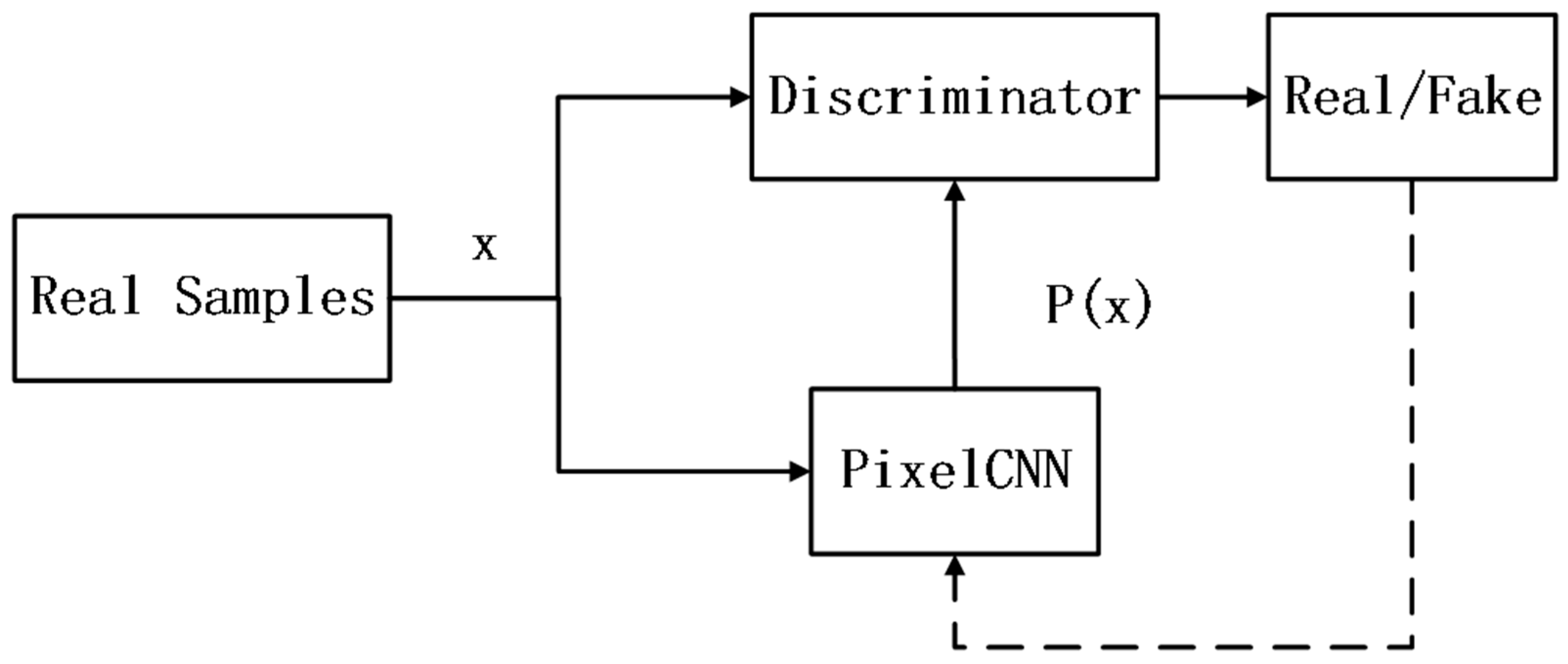
3. Credit Default Classification Process Based on PixelCNN-WGAN Algorithm

3.1. PixelCNN-WGAN Generative Model Construction

The PixelCNN-WGAN fusion model consists of a PixelCNN and a discriminator D. The training of the fusion model consists of two main processes: on the one hand, the real samples are transmitted as input data to the PixelCNN for learning the high-dimensional feature representations of the real image and capturing more information to reconstruct the data instances; on the other hand, the discriminator discriminates the input’s real samples and the fake samples generated by the PixelCNN, outputs the discrimination results, and feeds the results back to the PixelCNN. In this process, the PixelCNN and the discriminator continuously adjust their parameters to improve the learning ability and finally generate samples that are close to the real samples, as shown in Figure 2.

PixelCNN-WGAN uses a PixelCNN to implement the initial image generation and directly optimizes the model by maximizing the log-likelihood of the data, providing a more stable training process and image quality. The introduction of a PixelCNN makes up for the lack of a solid theoretical foundation for the original GAN to fully explain its working principle and the unstable situation in the training process.

3.2. Generator and Discriminator Network Structure

A PixelCNN accepts random noise as input, learns the conditional probability distribution of the corresponding pixels of the image data, and realizes the prediction of specific pixel values through neural networks. The PixelCNN model designed in this paper sets up three up-sampling convolutional layers to complete the feature extraction of the image and adds a batch normalization (BN) layer and a ReLU activation function to the output of each convolutional layer, which solves the problem of internal covariate bias, and the ReLU activation function introduces nonlinearities to the network and enhances the learning ability, which complement each other to improve the training stability and generalization ability of the network. The BN layer solves the internal covariate bias problem, and the ReLU activation function introduces nonlinearity to the network and enhances the learning ability, both of which complement each other to improve the training stability and generalization ability of the network, and a mask convolution layer is added after the convolutional layer, which further processes the image features through learning to generate pixel-level outputs, and finally generates a 10 × 10 × 1 grayscale image through the output layer. The specific structure is shown in Figure 3.

The input source of the discriminator consists of two parts: one is the generated samples generated by the PixelCNN, and the other is the real training samples. The discriminator sets a 3-layer downsampled convolutional layer and also adds a batch normalization layer and a ReLU activation function after each layer of convolution operation. The flattened spreading layer and fully connected layer are set up to extract the high feature representations for the subsequent classification, connecting with the BN layer and the ReLU activation function, and finally outputting the classification results through the second fully connected layer. The specific network structure design is shown in Figure 4.

3.3. Default Prediction Model Based on PixelCNN-WGAN Models

In this section, the default prediction model is designed based on the PixelCNN-WGAN model basis. Firstly, the original historical form data containing borrowers’ lending information are processed with data normalization and missing values, and the form image is transformed into a grayscale map using Python, including normal samples and default samples; then, the image data are balanced, and the grayscale maps of the default samples are inputted into the PixelCNN-WGAN model designed in Section 3.1, and the fusion model generates the image features by learning the number of generated samples needed for the experiment, and then the real samples are fused with the generated samples to obtain the balanced dataset needed for the experiment; the CNN [21], AlexNet [22], SqueezeNet [23], and MobileNetV2 [24] models, which are currently more effective in the field of image processing, are selected to complete the subsequent credit sample classification task. The classification models are tuned to achieve the optimal classification effect, and the corresponding specific values are output according to the evaluation indexes for subsequent analysis of the model effect. The specific flow chart is shown in Figure 5.

In the process of training the PixelCNN and the discriminator, the RMSprop optimizer was used to replace the original Adam optimizer. The Wasserstein distance is used to compute the loss between the distribution of real samples and the generated samples in the discriminator, and the truncation parameter is used to limit the parameters of the discriminator to a certain range to prevent the occurrence of the gradient vanishing or gradient explosion.

4. Experimental Results and Analysis

4.1. Experimental Environment and Hyperparameter Settings

The experiments in this paper were conducted on a 64-bit Windows 10 operating system using a 14-core Intel(R) Xeon(R) Platinum 8362 CPU @ 2.80 GHz processor, an NVIDIA GeForce RTX 4090 graphics card, and the programming language was Python, based on the Pytorch 2.0.1 deep learning framework. The number of iterations for the PixelCNN-WGAN model was set to 1000, the learning rate was 0.0001, the batch size was 64, and the Adam optimizer was selected; the parameters of the classification models CNN, AlexNet, SqueezeNet, and MobileNetV2 were set as shown in

Table 1. Parameter settings for different algorithms.

Algorithm	Parameterization
CNN	kernel_size:3,batch_size:128,pool_size:(2, 2)
AlexCNN	kernel_size:3,batch_size:64,dropout rate:0.5
SqueezeNet	kernel_size:3,fire module:kernel_size:1,dropout rate:0.5
MobileNetV2	inverted_residual_blockmodule:kernel_size:3

below.

4.2. Datasets and Data Preprocessing

The dataset selected in this paper is the historical data about borrowers’ lending information from the official website of LendingClub [25], and the experiment adopts the data from the first quarter of 2017, which contains a total of 96,779 data points of 145 variables of borrowers’ information. “Current” and “Fully Paid” in the dependent variable “loan_status” are recognized as normal samples, and the rest are default samples. Before the experiment, the raw data were normalized and processed with missing values, eliminating the indicators with more than half of the missing values, filling in the indicators with fewer missing values by using the multitude or the average, and transforming the subtypes of indicators into numerical indicators, and then obtaining a total of 86 indicators including the dependent variable “loan_status”, with a total of 87,691 indicators after the pretreatment. After preprocessing, a total of 86 indicators, including the dependent variable “loan_status”, were obtained, with a total of 87,691 data points, and the ratio of normal samples to default samples was about 9:1.

To analyze credit data, the tabular data were converted into grayscale charts with the help of a Python program. The blank metrics were filled with 0 values, and the data of each borrower were transformed into a grayscale graph of size 10 × 10 by referring to the method in the article of Hosaka [26], where the size of different metrics’ values was reflected by pixels. The transformation formula is as follows:

$$F_{ij}={\displaystyle \frac{v\left(x_{ij}\right)-m\left(x_i\right)}{\sigma \left(x_i\right)}}\times 100+128$$

(4)

where $x_{ij}$ denotes the row i and column j indicators, $\mathrm{v}(.)$ denotes the variance of the indicator values corresponding to all users, $m(.)$ denotes the mean, and $\mathsf{\sigma }$ denotes the standard deviation. The example grayscale plots of normal and default customers are obtained in Figure 6.

4.3. Evaluation of the Quality of the Generated Images

The Inception Score (IS) metric is currently used in many articles as a metric for evaluating the performance of GANs, and the IS mainly measures the clarity and diversity of the generated images, but since the metric is trained on the ImageNet dataset, the evaluation is biased toward that dataset and cannot calculate the similarity between the real samples and the generated images. To solve this problem, this paper chooses Frechet Inception Distance (FID) [27] as an index to measure the quality of the generated images, and the FID index quantitatively evaluates the similarity between the generated images and the real images by calculating the distance between their feature distributions, and the closer the distance is, the smaller the value of FID is, which indicates that the quality of the generated images is higher. The FID metric is less sensitive to outliers and small sample datasets, which makes it more reliable in practical applications. FID is defined as follows:

$${\mathrm{FID}}^2={‖{\mu }_1-{\mu }_2‖}^2+T_r\left({\sum }_1+{\sum }_2\right)-2\left({\sum }_1{\sum }_2^{1/2}\right)$$

(5)

where ${\mu }_1, {\mu }_2$ denotes the mean vector of the real and generated data distributions, in which ${‖{\mu }_1-{\mu }_2‖}^2$, calculated as the Euclidean distance between the two mean vectors, ${\mathsf{\Sigma }}_1$ and ${\mathsf{\Sigma }}_2$, denotes the covariance of the real and generated data distributions.

The original WGAN model and the PixelCNN-WGAN model designed in this paper are used to calculate the FID values with real default samples, and the results are obtained as in

Table 2. FID values for different generative models.

Model	FID Values	Time per Epoch/min
WGAN	152.70	0.73
PixelCNN-WGAN	92.02	2.15

. It can be seen that the FID values of the fusion generation model designed in this paper with real samples are smaller compared with WGANs, which proves that the images generated by the Pixel-WGAN are closer to the real images and have more details. Meanwhile, Table 2 also reflects the effect of adding a PixelCNN to the data enhancement task.

The training of deep learning is affected by a variety of factors such as equipment, data complexity, and resource allocation, as can be seen in Table 2. In terms of time cost, the time required for each iteration of the PixelCNN-WGAN model is 2.95 times longer than that of the WGAN model, due to the fact that firstly, this paper is based on a large dataset, with a large number of images being generated at a time of the order of tens of thousands of images, and secondly, the principle of PixelCNNs relies on pixel-by-pixel generation, and the time cost is higher than WGANs. At the same time, the high time cost also brings higher image quality. Comprehensively, it seems that the model proposed in this paper has a certain reference value, and the time cost and image quality will be further considered comprehensively in future work.

4.4. Evaluation Indicators

To comprehensively assess the model performance, the Accuracy and Area Under Curve (AUC) were used to evaluate the model classification. Accuracy indicates the ratio of the number of correctly predicted samples to the total number of samples, and the formula is as follows:

$$\mathrm{Accuracy}={\displaystyle \frac{\mathrm{TP}+\mathrm{TN}}{\mathrm{TP}+\mathrm{FN}+\mathrm{FP}+\mathrm{TN}}}$$

(6)

where true positive (TP) denotes samples that are normal and predicted to be normal as well, false positive (FP) denotes samples that are defaulted but predicted to be normal, true negative (TN) denotes samples that are defaulted and predicted to be defaulted as well, and false negative (FN) denotes samples that are normal but predicted to be defaulted.

AUC represents the area under the ROC curve. The ROC curve is a curve plotted with a false positive rate (FPR) as the horizontal coordinate and a true positive rate (TPR) as the vertical coordinate with Formulas (6) and (7) below. The higher the AUC, the better the model’s ability to distinguish between positive and negative samples, i.e., the better the model’s performance.

$$\mathrm{TPR}={\displaystyle \frac{\mathrm{TP}}{\mathrm{TP}+\mathrm{FN}}}$$

(7)

$$\mathrm{FPR}={\displaystyle \frac{\mathrm{FP}}{\mathrm{FP}+\mathrm{TN}}}$$

(8)

4.5. Comparison of Data Enhancement Effectiveness

To further verify the effectiveness of the PixelCNN-WGAN image generation model designed in this paper on balanced credit data, the original dataset and the balanced dataset are classified using four classification models commonly used in image classification, which include the CNN, AlexCNN, SqueezeNet, and MobileNetV2 models. The classification accuracy and AUC values under each model were further calculated, as shown in

Table 3. Effectiveness of balancing algorithms under different classification algorithms.

Algorithm	Original Dataset		Pixel-WGAN Balanced Dataset
	Accuracy	AUC	Accuracy	AUC
CNN	0.9392	0.6788	0.9749	0.9749
AlexCNN	0.9591	0.7873	0.9746	0.9746
SqueezeNet	0.9587	0.7874	0.9771	0.9771
MobileNetV2	0.9559	0.7947	0.9734	0.9734

.

As can be seen from Table 3, firstly, compared with multiple classification models, the accuracy and AUC index values of the CNN model on the original dataset are relatively low because the model structure of a CNN as the basic neural network model is relatively simple, and there are certain disadvantages in the classification effect compared with AlexCNN, SqueezeNet, and MobileNetV2. Secondly, compared with the original dataset, the balanced credit samples of the PixelCNN-WGAN generation model reflect higher classification accuracy and AUC values on the four classification algorithms, with the accuracy increased by 0.02–0.04 percentage points and the AUC value increased by 0.18–0.3 percentage points, indicating the feasibility of the image generation algorithm proposed in this paper in improving the classification effect of credit data. Also, a side-by-side comparison shows the effectiveness of PixelCNNs and WGANs in data enhancement.

5. Conclusions

In this paper, a PixelCNN-WGAN data enhancement algorithm applied to credit default classification is proposed, which combines two models in the field of image generation, utilizes the PixelCNN autoregressive model to generate pixels one by one by learning the conditional probability distribution, replaces the role of the generator in the Generative Adversarial Network, and combines with the WGAN that adds the Wasserstein distance to effectively avoid the problem of model gradient disappearance. This structure effectively avoids the problem of model gradient vanishing, realizes the data enhancement effect better than a single algorithm, and generates the grayscale image close to the real default sample. The experimental results on real datasets show that the data enhancement algorithm proposed in this paper embodies excellent effects on all four classification models, CNN, AlexNet, SqueezeNet, and MobileNetV2, and the balanced data are improved in terms of accuracy and AUC value compared with the original data, which proves the validity of the method in this paper in the field of credit evaluation.

Naturally, the proposed model PixelCNN-WGAN has certain limitations. Although the proposed model has better image generation results than WGANs when performing data augmentation, as shown in Table 2, it takes a long time to generate images because the PixelCNN model is based on the principle of pixel-by-pixel generation. This suggests that our proposed method still needs further improvement, which is the focus of future research. In future research, we will conduct a more in-depth theoretical study of PixelCNN to find a better dynamic balance between image quality and resource consumption.

References

1. Dal Pozzolo, A.; Boracchi, G.; Caelen, O.; Alippi, C.; Bontempi, G. Credit card fraud detection: A realistic modeling and a novel learning strategy. IEEE Trans. Neural Netw. Learn. Syst. 2017, 29, 3784–3797. [Google Scholar] [CrossRef] [PubMed]
2. Liu, Z.; Cao, W.; Gao, Z.; Bian, J.; Chen, H.; Chang, Y.; Liu, T.-Y. Self-paced ensemble for highly imbalanced massive data classification. In Proceedings of the 2020 IEEE 36th International Conference on Data Engineering (ICDE), Dallas, TX, USA, 20–24 April 2020; pp. 841–852. [Google Scholar]
3. Zhang, Q.; Zhu, Y.; Yang, M.; Jin, G.; Zhu, Y.; Chen, Q. Cross-to-merge training with class balance strategy for learning with noisy labels. Expert Syst. Appl. 2024, 249, 123846. [Google Scholar] [CrossRef]
4. Zhang, Q.; Lee, F.; Wang, Y.-g.; Ding, D.; Yao, W.; Chen, L.; Chen, Q. An joint end-to-end framework for learning with noisy labels. Appl. Soft Comput. 2021, 108, 107426. [Google Scholar] [CrossRef]
5. Chawla, N.V.; Bowyer, K.W.; Hall, L.O.; Kegelmeyer, W.P. SMOTE: Synthetic minority over-sampling technique. J. Artif. Intell. Res. 2002, 16, 321–357. [Google Scholar] [CrossRef]
6. Inoue, H. Data augmentation by pairing samples for images classification. arXiv 2018, arXiv:1801.02929. [Google Scholar]
7. Goodfellow, I.; Pouget-Abadie, J.; Mirza, M.; Xu, B.; Warde-Farley, D.; Ozair, S.; Courville, A.; Bengio, Y. Generative adversarial nets. Adv. Neural Inf. Process. Syst. 2014, 27, 2672–2680. [Google Scholar]
8. Ratliff, L.J.; Burden, S.A.; Sastry, S.S. Characterization and computation of local Nash equilibria in continuous games. In Proceedings of the 2013 51st Annual Allerton Conference on Communication, Control, and Computing (Allerton), Monticello, IL, USA,, 2–4 October 2013; pp. 917–924. [Google Scholar]
9. Hu, W.; Tan, Y. Generating adversarial malware examples for black-box attacks based on GAN. In Proceedings of the International Conference on Data Mining and Big Data, Beijing, China, 21–24 November 2022; pp. 409–423. [Google Scholar]
10. Yu, L.; Zhang, W.; Wang, J.; Yu, Y. Seqgan: Sequence generative adversarial nets with policy gradient. In Proceedings of the AAAI Conference on Artificial Intelligence, San Francisco, CA, USA, 4–9 February 2017. [Google Scholar]
11. Yang, Q.; Yan, P.; Zhang, Y.; Yu, H.; Shi, Y.; Mou, X.; Kalra, M.K.; Zhang, Y.; Sun, L.; Wang, G. Low-dose CT image denoising using a generative adversarial network with Wasserstein distance and perceptual loss. IEEE Trans. Med. Imaging 2018, 37, 1348–1357. [Google Scholar] [CrossRef] [PubMed]
12. Wang, J.; Yang, Z.; Zhang, J.; Zhang, Q.; Chien, W.-T.K. AdaBalGAN: An improved generative adversarial network with imbalanced learning for wafer defective pattern recognition. IEEE Trans. Semicond. Manuf. 2019, 32, 310–319. [Google Scholar] [CrossRef]
13. Arjovsky, M.; Chintala, S.; Bottou, L. Wasserstein generative adversarial networks. In Proceedings of the International Conference on Machine Learning, Sydney, Australia, 6–11 August 2017; pp. 214–223. [Google Scholar]
14. Zhang, X.; Yu, L.; Yin, H.; Lai, K.K. Integrating data augmentation and hybrid feature selection for small sample credit risk assessment with high dimensionality. Comput. Oper. Res. 2022, 146, 105937. [Google Scholar] [CrossRef]
15. Cui, J.; Zhang, Y.; Men, J.; Wu, L. Utilizing Wasserstein Generative Adversarial Networks for Enhanced Hyperspectral Imaging: A Novel Approach to Predict Soluble Sugar Content in Cherry Tomatoes. LWT 2024, 206, 116585. [Google Scholar] [CrossRef]
16. Zekrifa, D.M.S.; Lamani, D.; Chaitanya, G.K.; Kanimozhi, K.; Saraswat, A.; Sugumar, D.; Vetrithangam, D.; Koshariya, A.K.; Manjunath, M.S.; Rajaram, A. Advanced deep learning approach for enhancing crop disease detection in agriculture using hyperspectral imaging. J. Intell. Fuzzy Syst. 2024, 46, 3281–3294. [Google Scholar] [CrossRef]
17. Fan, H.; Ma, J.; Zhang, X.; Xue, C.; Yan, Y.; Ma, N. Intelligent data expansion approach of vibration gray texture images of rolling bearing based on improved WGAN-GP. Adv. Mech. Eng. 2022, 14, 16878132221086132. [Google Scholar] [CrossRef]
18. Zhao, C.; Zhang, L.; Zhong, M. An Improved WGAN-Based Fault Diagnosis of Rolling Bearings. In Proceedings of the 2022 IEEE International Conference on Sensing, Diagnostics, Prognostics, and Control (SDPC), Chongqing, China, 5–7 August 2022; pp. 322–327. [Google Scholar]
19. Van Den Oord, A.; Kalchbrenner, N.; Kavukcuoglu, K. Pixel recurrent neural networks. In Proceedings of the International Conference on Machine Learning, New York City, NY, USA, 19–24 June 2016; pp. 1747–1756. [Google Scholar]
20. Liao, W.; Ge, L.; Bak-Jensen, B.; Pillai, J.R.; Yang, Z. Scenario prediction for power loads using a pixel convolutional neural network and an optimization strategy. Energy Rep. 2022, 8, 6659–6671. [Google Scholar] [CrossRef]
21. LeCun, Y.; Bottou, L.; Bengio, Y.; Haffner, P. Gradient-based learning applied to document recognition. In Proceedings of the IEEE; IEEE: Seattle, WA, USA, 15 May 1998; pp. 2278–2324. [Google Scholar]
22. Krizhevsky, A.; Sutskever, I.; Hinton, G.E. Imagenet classification with deep convolutional neural networks. Adv. Neural Inf. Process. Syst. 2012, 25. [Google Scholar] [CrossRef]
23. Iandola, F.N.; Han, S.; Moskewicz, M.W.; Ashraf, K.; Dally, W.J.; Keutzer, K. SqueezeNet: AlexNet-level accuracy with 50x fewer parameters and <0.5 MB model size. arXiv 2016, arXiv:1602.07360. [Google Scholar]
24. Sandler, M.; Howard, A.; Zhu, M.; Zhmoginov, A.; Chen, L.-C. Mobilenetv2: Inverted residuals and linear bottlenecks. In Proceedings of the IEEE Conference on Computer Vision and Pattern Recognition, Salt Lake City, UT, USA, 18–23 June 2018; pp. 4510–4520. [Google Scholar]
25. LendingClub Home Page. Available online: https://www.lendingclub.com/info/download-data.action (accessed on 17 July 2023).
26. Hosaka, T. Bankruptcy prediction using imaged financial ratios and convolutional neural networks. Expert Syst. Appl. 2019, 117, 287–299. [Google Scholar] [CrossRef]
27. Heusel, M.; Ramsauer, H.; Unterthiner, T.; Nessler, B.; Hochreiter, S. Gans trained by a two time-scale update rule converge to a local nash equilibrium. Adv. Neural Inf. Process. Syst. 2017, 30. [Google Scholar]
Figure 1. GAN structure diagram.
Electronics 13 03419 g001
Figure 2. PixelCNN-WGAN model structure diagram.
Electronics 13 03419 g002
Figure 3. Structure of PixelCNN.
Electronics 13 03419 g003
Figure 4. Structure of discriminator.
Electronics 13 03419 g004
Figure 5. Pixel-WGAN default prediction flowchart.
Electronics 13 03419 g005
Figure 6. A grayscale map of credit data. There are obvious differences in the images corresponding to the normal samples and the default samples in some areas.
Electronics 13 03419 g006