Bio-Inspired Multimodal Motion Gait Control of Snake Robots with Environmental Adaptability Based on ROS

Abstract

Snake robots have broad application potential, but their motion-control and motion-planning problems are extremely challenging due to the high redundancy of degrees of freedom (DoFs), and the lack of complete system tools further hinders the research of snake robots. In this paper, a coordinate system and a kinematic model were established based on the D-H method for snake robots. The rhythm-generation model for multimodal motion gait and a novel sliding-window five-point interpolation-derivative model were proposed based on a bio-inspired central pattern generator (CPG) model. A prototype and simulator were constructed based on the designed snake robot models to achieve the multimodal motion gait for the snake robot and improve its environmental adaptability. Furthermore, a novel structure–drive–perception–control integration snake robot system (SnakeSys) was built based on the robot-operating system (ROS). Finally, the effectiveness, feasibility, and accuracy of the kinematic model and control model in motion control and information perception were verified through simulations and experiments. We open sourced SnakeSys so that relevant researchers or developers can directly utilize or further develop it.

1. Introduction

Snake robots are highly redundant mobile robots designed by humans to mimic natural snakes [1]. They are usually composed of multiple joint modules with the same structure in series, with a number typically ranging from 10 to 30, and each joint corresponds to a control DoF [2]. The control DoFs of snake robots are much greater than their motion DoFs, with only six motion DoFs corresponding to three positional DoFs and three rotational DoFs. Snake robots have slender body structures and strong environmental adaptability and can perform tasks in complex and unstructured environments such as underwater, land, and pipelines [3]. Compared with traditional wheeled and legged mobile robots, snake robots have flexible and diverse movement gaits, such as creeping locomotion (CL) [4], traveling wave locomotion (TWL) [5], side winding locomotion (SWL) [6], arc rolling locomotion (ARL) [7], and spiral rolling locomotion (SRL) [8]. Therefore, they have great application potential in disaster search and rescue, field reconnaissance, interstellar exploration, and information collection [9]. However, the high redundancy DoF of snake robots makes their dynamics, motion control, and motion planning extremely challenging. For example, it is often difficult to obtain inverse solutions for the kinematics and dynamics of snake robots, and their motion mechanism based on environmental interactions also leads to highly coupled and nonlinear dynamic models, making traditional robot-control methods difficult to apply to snake robots [2,10].

The serial joint structure and diverse application scenarios of snake robots greatly increase the difficulty of designing their body structure. Professor Hirose was the first to research snake robots. He and his team developed a series of snake robots, ACM-R3 [11], ACM-R8 [12], ACM-S1 [13], etc., with the joint types from parallel to orthogonal and the movement ranges from land to amphibious. Zuo et al. [14] designed a snake robot based on the origami principle, which has a more lightweight and flexible replacement comparing traditional structures. Bi et al. [15] designed a Worm-Snake-Inspired Metameric (WSIM) robot with multimodal motion capability, suitable for open and narrow terrains. Qi et al. [16] designed a pneumatic soft snake robot with a modular structure and 3D printing molding; it can achieve TWL gait and move in complex and restricted environments based on four air channels. Gautreau et al. [17] used the design method based on a hybrid continuum cable-driven robot (HCDR), replaced the connection between muscles and vertebrae in snakes with cable drive, and provided good fluidity and locomotion for the snake robot. In engineering, the most practical joint type of snake robot is the orthogonal joint, which can achieve the three-dimensional motion gait of snake robots and have the advantages of high stability and strength [9]. However, snake robots still face problems such as low load, high power consumption, and low endurance.

Due to the high redundant DoF, the control for snake robots is usually based on pre-designed joint rhythm patterns to achieve their motion. There are two classic control methods: the curve-based method and the CPG-based method. The curve-based method has a serpenoid curve [18], serpentine curve [19], backbone curve [20,21], etc. However, these curve-based methods are not flexible enough and are prone to joint mutation problems when adjusting control parameters or changing motion gait. The CPG-based method was inspired and established by biology. CPG models usually consist of multiple neurons or nonlinear oscillators to couple a high-dimensional distributed nonlinear oscillation network. This network generates rhythmic signals through self-excited oscillations, which can be directly used as control inputs [22]. The CPG is usually composed of unit models of first-order or second-order differential equations, and it can still produce a smooth output when parameters undergo sudden changes, effectively solving the problem of joint mutation. The CPG model has multimodal characteristics, distributed characteristics, and inherent limit cycle characteristics. One CPG model can generate multimodal control signals to achieve different motion gaits for snake robots [23].

CPG models often use nonlinear oscillators, such as Hopf [24], Kuramoto [25], Van der Pol (VDP) [26], Delayed Half Center Oscillator (DHCO) [27,28,29], Rayleigh [30], etc. Oscillators form phase interlocks through coupling to generate rhythmic signals. Manzoo and Choi et al. [31] designed a unified CPG model based on Kuramoto oscillators for the snake robot with active wheels and passive joints to realize motion gaits for serpentine locomotion, rectilinear locomotion, and concertina locomotion. Zhang et al. [32] constructed a dual-chain CPG model based on Hopf oscillators, achieving motion gaits such as lateral undulation and rectilinear motion. Wang et al. [33] constructed a diffusion-coupled connected double-chain CPG model based on Hopf oscillators and demonstrated the stability of the CPG model using partial contraction theory. They achieved motion gaits such as serpentine locomotion, concertina locomotion, and sidewinding locomotion for the snake robot. Fukuoka et al. [34] used decoupled neural oscillators in conjunction with appropriate mechanical designs for snake robots and achieved enhanced robustness, variability, and independent local propulsion. However, the rhythm signals generated by the CPG are mostly designed based on the gaits of biological snakes, and there is no more optimization design for the mechanical performance of snake robots. At the same time, further research is needed to achieve more complex motion-adaptive control by combining environmental information and the motion state of snake robots.

The research on robots involves multiple interdisciplinary fields such as control, communication, computer science, mathematics, and mechanics [35]. Therefore, many scholars and developers have developed robot tools and frameworks to facilitate the study of robots. ROS2 [36,37] is an open-source robot-operating system and the next-generation version of ROS1. ROS2 supports multiple robot systems, multiple languages, cross-platforms, an improved real-time performance, and communication mechanisms, and it includes hardware abstraction, device drivers, message passing, and package management. Gazebo [38] is an open-source robot-simulation software that can simulate robots in real environments, including physical, sensor, environmental, etc. Gazebo includes ODE, Bullet, Simbody, and DART dynamic engines, providing precise simulation for robots, and it can be tightly integrated with the ROS to achieve joint simulation.

Sanfilippo et al. [39] designed SnakeSIM based on ROS1 and Gazebo, which is divided into three levels: perception, motion planning, and high-level control, aiming to simulate perception-driven obstacle-aided locomotion (POAL) for snake robots. However, SnakeSIM has not implemented the snake robot prototype and different motion gaits. Ni et al. [40] designed a system, which includes a human–computer interaction layer, head controller layer, and joint layer. The system communicates between the host computer and the snake robot based on TCP/IP, and it controls the movement of the snake robot through the interactive interface designed by Microsoft Foundation Classes (MFC). However, due to the lack of existing robot frameworks, the system requires extremely high skill requirements for researchers to develop and expand further. Zhou et al. [41] constructed a real-time control system based on Xenomai and combined it with ROS1, which can run real-time applications based on hardware control and non-real-time applications based on ROS1. To the best of our knowledge, there are almost no open-source frameworks and tools related to snake robots. Research on snake robots often requires research teams to master multiple forms of knowledge and skills, and there is weak interest in snake robot research [42,43]. This is also an important factor that explains why there are still many unresolved control and planning problems for snake robots, which cannot be widely applied in practical engineering.

The content of this paper is organized to deal with these problems. In Section 2, we establish a coordinate system including sensors and a kinematic model for the snake robot with orthogonal joints. In Section 3, a new sliding-window five-point interpolation-derivative model is proposed, and a multimodal motion-gait-control model is constructed for the snake robot based on the bio-inspired CPG model. In Section 4, structures of snake robots are designed, a simulator of the snake robot is built based on Gazebo, and a prototype of the snake robot is realized based on Snake Robot III. Based on this, a novel open-source SnakeSys for structure–drive–perception–control integration is constructed based on the ROS. In Section 5, the effectiveness, feasibility, and accuracy of SnakeSys in motion control and information perception are verified through simulations and experiments. In Section 6, the research of this paper is summarized and analyzed, and the shortcomings and problems are discussed.

2. Kinematic Model for Snake Robots with Orthogonal Joints

Due to the lack of a leg–foot structure, snake robots achieve their movement through the contact between each linkage and the environment, as well as their body wave rhythm. The collision or contact between each linkage and the environment, and the pattern of the body wave rhythm of the snake robot, are all related to kinematics. Kinematics describes the pose of the snake robot and the relative relationships among its linkages. To address this, we establish a coordinate system for the snake robot and then build its kinematic model using the Denavit–Hartenberg (D-H) method.

2.1. Coordinate System for Snake Robots

A snake robot with n orthogonal joints has N rotating pairs, and $N=2n$. The rotating pair connects adjacent joint linkages, and the directions of adjacent rotating pairs are perpendicular. The number of orthogonal joints of snake robots will be designed to be very large to ensure that they have sufficient flexibility and maneuverability during movement. The slender body structure of snake robots limits the internal space of their joint modules. Due to the small size and light weight of visual and inertial sensors, they are suitable as the main sensors for snake robots to achieve their navigation, localization, and environmental perception capabilities. Therefore, considering the sensors and high DoFs of snake robots, we construct its coordinate system, as shown in Figure 1.

In Figure 1, the cameras and the inertial measurement unit (IMU) are fixed on the head of the snake robot, and the frames of each camera are $C_1$ and $C_2$. The IMU frame is I. The frames of the base linkage and each joint linkage are B, $J_1$, $J_2$, $J_3$, …, $J_N$. The transformations from B to $C_1$, B to $C_2$, and B to I are $T_{B,C_1}$, $T_{B,C_2}$, and $T_{B,I}$, respectively, which are obtained through calibration. The transformations from B to $J_1$, $J_1$ to $J_2$, ⋯, $J_{N-1}$ to $J_N$ are $T_{B,J_1}$, $T_{J_1,J_2}$, ⋯, $T_{J_{N-1},J_N}$, respectively, which are obtained through the kinematic model.

2.2. Kinematic Model for Snake Robot Body

Assuming that the joint linkage is rigid and will not deform during movement, according to the Craig agreement, the parameters and coordinate system of linkage are shown in Figure 2, and the parameters of all joint linkages of the snake robot are shown in

Table 1. Parameters of joint linkages of the snake robot.

Index i	${\mathit{\alpha }}_{\mathit{i}-1}$	${\mathit{a}}_{\mathit{i}-1}$	${\mathit{d}}_{\mathit{i}}$	${\mathit{\theta }}_{\mathit{i}}$
1	0	0	0	$-{\varphi }_1+\pi /2$
2	$-\pi /2$	$l_1$	0	$-{\varphi }_2$
3	$\pi /2$	$l_2$	0	$-{\varphi }_3$
4	$-\pi /2$	$l_3$	0	$-{\varphi }_4$
5	$\pi /2$	$l_4$	0	$-{\varphi }_5$
⋮	⋮	⋮	⋮	⋮
$N-1$	$-\pi /2$	$l_{N-2}$	0	$-{\varphi }_{N-1}$
N	$\pi /2$	$l_{N-1}$	0	$-{\varphi }_N$

[44]. Using the D-H method and according to Figure 1 and Figure 2, the transformation $T_{B,J_i}$ from the base frame B to the joint linkage frame $J_i$ of the snake robot is

$$T_{B,J_i}=T_{B,J_1}\prod _{j=2}^i{T}_{J_{j-1},J_j}$$

(1)

where

$$T_{J_{i-1},J_i}=\left[\begin{array}{cccc}cos{\theta }_i& -sin{\theta }_i& 0& a_{i-1}\\ cos{\alpha }_{i-1}sin{\theta }_i& cos{\alpha }_{i-1}cos{\theta }_i& -sin{\alpha }_{i-1}& -d_{i}sin{\alpha }_{i-1}\\ sin{\alpha }_{i-1}sin{\theta }_i& sin{\alpha }_{i-1}cos{\theta }_i& cos{\alpha }_{i-1}& d_{i}cos{\alpha }_{i-1}\\ 0& 0& 0& 1\end{array}\right].$$

(2)

Letting $T_{B,J_1}=T_{J_0,J_1}$ and substituting the parameters in Table 1 into Equation (1), due to the repetitive and orthogonal structure of the snake robot, i.e., $l_1=l_2=\cdots =l_{N-1}=l$, the simplified transformation can be obtained and is represented as

$$T_{J_{i-1},J_i}=\left\{\begin{array}{c}\left[\begin{array}{cccc}sin{\varphi }_i& -cos{\varphi }_i& 0& 0\\ cos{\varphi }_i& sin{\varphi }_i& 0& 0\\ 0& 0& 1& 0\\ 0& 0& 0& 1\end{array}\right],i=1\hfill \\ \left[\begin{array}{cccc}cos{\varphi }_i& sin{\varphi }_i& 0& l\\ 0& 0& -1& 0\\ -sin{\varphi }_i& cos{\varphi }_i& 0& 0\\ 0& 0& 0& 1\end{array}\right],i\in \mathrm{odd}\hfill \\ \left[\begin{array}{cccc}cos{\varphi }_i& sin{\varphi }_i& 0& l\\ 0& 0& 1& 0\\ sin{\varphi }_i& -cos{\varphi }_i& 0& 0\\ 0& 0& 0& 1\end{array}\right],i\in \mathrm{even}\hfill \end{array}\right..$$

(3)

Equations (1) and (3) describe the geometric state of the snake robot, and they can be used to calculate the self-collision of the snake robot to avoid self-interference among joint linkages, providing a theoretical basis for motion planning and gait control for snake robots.

2.3. Kinematic Model Based on Visual SLAM

To solve the pose of the snake robot in the motion environment and the transformations between each joint linkage and the environment, we estimate the camera pose, i.e., $T_{W,C_1}$, in real time during the motion of the snake robot using the Visual SLAM algorithm. At the same time, the Visual SLAM can create a point cloud map for the environment. Assuming that the frames corresponding to all map points are $P_1$, $P_2$, $P_3$, ⋯, $P_s$, the transformations from the world frame to each point cloud frame are $T_{W,P_1}$, $T_{W,P_2}$, $T_{W,P_3}$, ⋯, $T_{W,P_s}$.

The pose of the snake robot in the environment, i.e., $T_{W,B}$, is

$$T_{W,B}=T_{W,C_1}·T_{C_1,B}=T_{W,C_1}·T_{B,C_1}^{-1}.$$

(4)

The pose of the i-th joint linkage in the environment, i.e., $T_{W,J_i}$ is

$$T_{W,J_i}=T_{W,B}·T_{B,J_i}.$$

(5)

The transformation $T_{J_i,P_j}$ from the i-th joint linkage to the j-th map point is

$$T_{J_i,P_j}=T_{J_i,W}·T_{W,P_j}=T_{W,J_i}^{-1}·T_{W,P_j}.$$

(6)

According to the transformation $T_{J_i,P_j}$, the pose between each joint linkage and environmental objects can be obtained, which can be used for collision detection and obstacle avoidance between the snake robot and environment objects.

3. Multimodal Motion Gait Control for Snake Robots

The diverse motion gaits enable snake robots to adapt to complex environments, while the high redundancy of snake robots makes the control problem of their motion gait extremely challenging. Therefore, it is necessary to coordinate the motion of the control DoFs corresponding to each joint of the snake robot through a pre-designed body wave rhythm. We establish a gait-control model for the snake robot based on a bio-inspired CPG model to achieve different motion gaits and improve its environmental adaptability.

3.1. Rhythm Generation Based on a Bio-Inspired CPG Model

Due to the self-excited oscillation characteristics of the CPG model, which can spontaneously and continuously generate rhythmic signals, we can use these signals as joint-control signals for snake robots to achieve their body rhythm wave and drive their movement, as shown in Figure 3. In our previous research, we proposed an improved Hopf oscillator and its coupling model for the CPG model to achieve motion control of the snake robot [45]. The improved Hopf oscillator of the CPG model is

$$\mathcal{H}\left({}^o\mathit{x}\right)={}^o\dot{\mathit{x}}=\left[{}^o{\mathit{M}}_{\omega }+{}^o{\mathit{M}}_{\gamma }\right]{}^o\widehat{\mathit{x}}$$

(7)

$${}^o{\mathit{M}}_{\omega }=\omega \left[\begin{array}{cc}0& -1\\ 1& 0\end{array}\right]\in {\mathbb{R}}^{2\times 2}$$

(8)

$${}^o{\mathit{M}}_{\gamma }={\xi }_{\gamma }\left[\begin{array}{cc}1& 0\\ 0& 1\end{array}\right]\in {\mathbb{R}}^{2\times 2}$$

(9)

$${}^o\widehat{\mathit{x}}={}^o\mathit{x}-{}^o{\mathit{x}}_c$$

(10)

$${\xi }_{\gamma }=\left\{\begin{array}{c}\lambda \mathcal{S}(e_{\gamma },k_{\gamma }),\sigma >0\mathrm{and}{e}_{\gamma }<0\hfill \\ \lambda e_{\gamma },\mathrm{others}\hfill \end{array}\right.$$

(11)

$$\mathcal{S}(x,k)={\displaystyle \frac{2}{1+e^{-kx}}}-1$$

(12)

$$e_{\gamma }\left(\gamma \right)=\sigma -{\displaystyle \frac{{\gamma }^2}{{\rho }^2}}$$

(13)

$${\gamma }^2={|{}^o\widehat{\mathit{x}}|}^2={\widehat{u}}^2+{\widehat{v}}^2$$

(14)

where $u_c$ and $v_c$ are constants and $\rho >0$. $\lambda$ affects the convergence rate of the oscillator toward the limit cycle. When $\sigma >0$, the oscillator converges to the limit cycle, and when $\sigma <0$, the oscillator converges to the equilibrium point. $\mathcal{S}(x,k)$ is the amplitude optimization function, where k is the optimization coefficient and it is a constant. As the value of k increases, the amplitude variation in the oscillator becomes less smooth, while the smaller the value of k, the slower the convergence speed of the oscillator. Therefore, this paper sets $k=1$ to ensure that the oscillator has good dynamic characteristics.

Similar to the connections between biological neurons, different Hopf oscillators form phase interlocks through coupling. The coupling model between the i-th oscillator and all other oscillators is

$${\dot{\mathit{x}}}_i=\mathcal{H}\left({\mathit{x}}_i\right)-\alpha \sum _{j=1,j\ne i}^N{w}_{i,j}({\widehat{\mathit{x}}}_i-{\mathit{T}}_{i,j}{\widehat{\mathit{x}}}_j)$$

(15)

$${\mathit{T}}_{i,j}={\displaystyle \frac{\sqrt{{\sigma }_i}{\rho }_i}{\sqrt{{\sigma }_j}{\rho }_j}}·\left[\begin{array}{cc}cos\left({\varphi }_{i,j}\right)& -sin\left({\varphi }_{i,j}\right)\\ sin\left({\varphi }_{i,j}\right)& cos\left({\varphi }_{i,j}\right)\end{array}\right]\in {\mathbb{R}}^{2\times 2}$$

(16)

where ${\sigma }_i>0$ and ${\sigma }_j>0$. $\mathcal{H}\left({\mathit{x}}_i\right)$ is the i-th Hopf oscillator. ${\rho }_i$ and ${\rho }_j$ are positive in the counterclockwise direction and negative in the clockwise direction. ${\varphi }_{i,j}$ is the i-th row and j-th column element of $\mathbf{\Phi }$, and $\mathbf{\Phi }\in {\mathbb{R}}^{N\times N}$.

According to the Hopf oscillator model in Equation (7) and the coupling model in Equation (15), the CPG model is

$$\left\{\begin{array}{cc}\hfill \dot{\mathit{x}}& =\left({\mathit{M}}_{\omega }+{\mathit{M}}_{\gamma }+{\mathit{M}}_c\right)\widehat{\mathit{x}}\hfill \\ \hfill \mathit{y}& ↤\mathit{Ex}\hfill \end{array}\right.$$

(17)

where $\mathit{x}\in {\mathbb{R}}^{2N}$ and $\widehat{\mathit{x}}\in {\mathbb{R}}^{2N}$. $\mathit{y}\in {\mathbb{R}}^N$ is the desired joint-position-control sequence of the snake robot, which is mapped from the state variables reduced by the $\mathit{E}$ matrix, and

$$\mathit{E}=\left[\begin{array}{ccccccc}1& 0& & & \cdots & & \\ & & 1& 0& \cdots & & \\ ⋮& ⋮& ⋮& ⋮& \ddots & ⋮& ⋮\\ & & & & \cdots & 1& 0\end{array}\right]\in {\mathbb{R}}^{N\times 2N}.$$

(18)

${\mathit{M}}_{\omega }\in {\mathbb{R}}^{2N\times 2N}$ and ${\mathit{M}}_{\gamma }\in {\mathbb{R}}^{2N\times 2N}$ in Equation (17) are high-demensional stacks of ${}^o{\mathit{M}}_{\omega }$ in Equation (8) and ${}^o{\mathit{M}}_{\gamma }$ in Equation (9). ${\mathit{M}}_c$ maintains a specific phase difference among oscillators to form phase interlocks, as

$${\mathit{M}}_c=-\alpha {\mathit{D}}^{-1}\mathit{LD}\in {\mathbb{R}}^{2N\times 2N}$$

(19)

where

$$\mathit{D}=\left[\begin{array}{cccc}{\mathit{D}}_{1,1}& & \cdots & \\ & {\mathit{D}}_{2,2}& \cdots & \\ ⋮& ⋮& \ddots & ⋮\\ & & \cdots & {\mathit{D}}_{N,N}\end{array}\right]\in {\mathbb{R}}^{2N\times 2N}$$

(20)

$$\mathit{L}=\left[\begin{array}{cccc}{\mathit{L}}_{1,1}& {\mathit{L}}_{1,2}& \cdots & {\mathit{L}}_{1,N}\\ {\mathit{L}}_{2,1}& {\mathit{L}}_{2,2}& \cdots & {\mathit{L}}_{2,N}\\ ⋮& ⋮& \ddots & ⋮\\ {\mathit{L}}_{N,1}& {\mathit{L}}_{N,2}& \cdots & {\mathit{L}}_{N,N}\end{array}\right]\in {\mathbb{R}}^{2N\times 2N}$$

(21)

$${\mathit{D}}_{i,j}=\left\{\begin{array}{c}{\mathit{T}}_{1,i},i=j\hfill \\ {\mathbf{0}}_2,i\ne j\hfill \end{array}\right.$$

(22)

$${\mathit{L}}_{i,j}=\left\{\begin{array}{c}\left(\sum _{k=1,k\ne i}^N{w}_{i,k}\right)·{\mathit{I}}_2,i=j\hfill \\ -w_{i,j}·{\mathit{I}}_2,i\ne j\hfill \end{array}\right..$$

(23)

3.2. Generative Control for Multimodal Motion Gait

Selecting different motion gaits based on the characteristics of various motion environments can effectively improve the environmental adaptability and motion maneuverability of snake robots. The amplitude, frequency, and phase differences among oscillators determine the output waveform mode of the CPG model. By changing the corresponding control parameters, the CPG model can generate multimodal waveforms and control the snake robot to achieve different motion gaits. For the CL, TWL, and SWL motion gaits of snake robots, the control functions are

$${\varphi }_{i,j}=\left\{\begin{array}{c}{\displaystyle \frac{2K_n\pi }{n}},i\in \mathrm{yaw},j\in \mathrm{yaw},j-i=2\hfill \\ {\displaystyle \frac{\pi }{2}},i\in \mathrm{yaw},j\in \mathrm{pitch},j-i=1\hfill \\ {\displaystyle \frac{2K_n\pi }{n}},i\in \mathrm{pitch},j\in \mathrm{pitch},j-i=2\hfill \end{array}\right.$$

(24)

$${\rho }_i=\left\{\begin{array}{c}2a_{y}sin\left({\displaystyle \frac{K_n\pi }{n}}\right),i\in \mathrm{yaw}\hfill \\ 0.1,i\in \mathrm{pitch}\hfill \end{array}\right.$$

(25)

$${\rho }_i=\left\{\begin{array}{c}0.1,i\in \mathrm{yaw}\hfill \\ 2a_{p}sin\left({\displaystyle \frac{K_n\pi }{n}}\right),i\in \mathrm{pitch}\hfill \end{array}\right.$$

(26)

$${\rho }_i=\left\{\begin{array}{c}2a_{y}sin\left({\displaystyle \frac{K_n\pi }{n}}\right),i\in \mathrm{yaw}\hfill \\ 2a_{p}sin\left({\displaystyle \frac{K_n\pi }{n}}\right),i\in \mathrm{pitch}\hfill \end{array}\right.$$

(27)

where Equations (25)–(27) are used to achieve CL, TWL, and SWL gaits, respectively.

For the ARL gait, the snake robot forms a continuously rolling arc, and its control functions are

$${\varphi }_{i,j}=\left\{\begin{array}{c}0,i\in \mathrm{yaw},j\in \mathrm{yaw},j-i=2\hfill \\ {\displaystyle \frac{\pi }{2}},i\in \mathrm{yaw},j\in \mathrm{pitch},j-i=1\hfill \\ 0,i\in \mathrm{pitch},j\in \mathrm{pitch},j-i=2\hfill \end{array}\right.$$

(28)

$${\rho }_i=2{\displaystyle \frac{l}{r_a}},i\in \mathrm{yaw}\mathrm{or}i\in \mathrm{pitch}$$

(29)

For the SRL gait, the snake robot forms a spiral that can climb along the outer or inner surface of the cylinder, and its control functions are

$${\varphi }_{i,j}=\left\{\begin{array}{c}\overline{\tau }l,i\in \mathrm{yaw},j\in \mathrm{yaw},j-i=2\hfill \\ {\displaystyle \frac{\pi }{2}},i\in \mathrm{yaw},j\in \mathrm{pitch},j-i=1\hfill \\ \overline{\tau }l,i\in \mathrm{pitch},j\in \mathrm{pitch},j-i=2\hfill \end{array}\right.$$

(30)

$${\rho }_i={\displaystyle \frac{2\overline{\kappa }}{\overline{\tau }}}sin\left(\overline{\tau }l\right),i\in \mathrm{yaw}\mathrm{or}i\in \mathrm{pitch}$$

(31)

$$\left\{\begin{array}{c}\overline{\kappa }={\displaystyle \frac{r_s}{r_s^2+p_s^2}}\hfill \\ \overline{\tau }={\displaystyle \frac{p_s}{r_s^2+p_s^2}}\hfill \end{array}\right.$$

(32)

$$\sqrt{{\left(2\pi r_s{S}_n\right)}^2+{\left(2\pi p_s\right)}^2}=(2n+1)l$$

(33)

where $2\pi p_s$ represents the axial distance of the overall spiral curve.

By selecting the corresponding control function and its control parameters, such as $K_n$, $a_y$, $a_p$, $r_a$, etc., the parameters ${\rho }_i$ and ${\varphi }_{i,j}$ can be obtained for the CPG model, thereby achieving different motion gaits and its smooth switching of the snake robot.

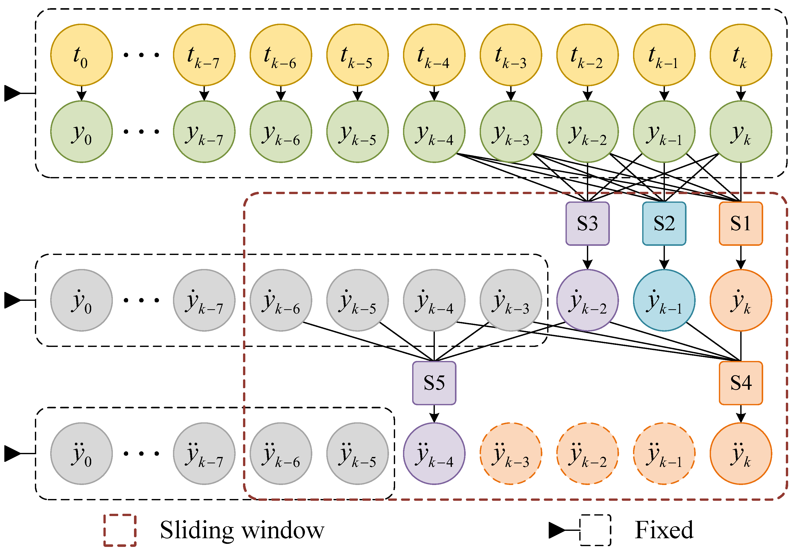
3.3. Sliding-Window Interpolation-Derivative Model for Rhythm

Considering that snake robots may simultaneously control joint actuators based on physical quantities such as position, velocity, or acceleration of joints, we use numerical methods to numerically differentiate the discrete rhythm output of the CPG model and obtain its first and second derivatives, corresponding to the velocity and acceleration of joints, respectively. The rhythm output of the CPG model is a time-discrete control sequence. We assume that at different times $t_0,t_1,t_2,\cdots ,t_k$, one oscillator output of the CPG model corresponds to joint positions $y_0,y_1,y_2,\cdots ,y_k$.

We introduce the Lagrange interpolation polynomial and obtain the corresponding first-order derivative by taking its derivative. For data points $(t_0,y_0)$, $(t_1,y_1)$, ⋯, $(t_m,y_m)$, the Lagrange interpolation polynomial is

$${\mathcal{L}}_m\left(t\right)={\displaystyle \sum _{i=0}^m}{\displaystyle \frac{{\displaystyle \prod _{j=0,j\ne i}^m}\left(t-t_j\right)}{{\displaystyle \prod _{j=0,j\ne i}^m}\left(t_i-t_j\right)}}{y}_i.$$

(34)

According to Equation (34), its first-order derivative is

$${\dot{\mathcal{L}}}_m\left(t\right)={\displaystyle \frac{\mathrm{d}{\mathcal{L}}_m\left(t\right)}{\mathrm{d}t}}=\sum _{i=0}^m{\displaystyle \frac{{\displaystyle \sum _{j=0,j\ne i}^m}{\displaystyle \prod _{d=0,d\ne j,d\ne i}^m}\left(t-t_d\right)}{{\displaystyle \prod _{j=0,j\ne i}^m}\left(t_i-t_j\right)}}{y}_i.$$

(35)

To calculate accuracy and efficiency, we adopt the five-point interpolation-derivative method. Substituting the five data points $(t_0,y_0)$, $(t_1,y_1)$, ⋯, $(t_4,y_4)$ into Equation (35) to obtain their first-order derivatives results in

$${\dot{y}}_0\approx {\dot{\mathcal{L}}}_4\left(t_0\right)=\sum _{i=0}^4\left(\left(\sum _{j=0,j\ne i}^4\prod _{d=0,d\ne j,d\ne i}^4\left(t_0-t_d\right)\right)\prod _{j=0,j\ne i}^4{\left(t_i-t_j\right)}^{-1}\right)y_i$$

(36)

$${\dot{y}}_1\approx {\dot{\mathcal{L}}}_4\left(t_1\right)=\sum _{i=0}^4\left(\left(\sum _{j=0,j\ne i}^4\prod _{d=0,d\ne j,d\ne i}^4\left(t_1-t_d\right)\right)\prod _{j=0,j\ne i}^4{\left(t_i-t_j\right)}^{-1}\right)y_i$$

(37)

$${\dot{y}}_2\approx {\dot{\mathcal{L}}}_4\left(t_2\right)=\sum _{i=0}^4\left(\left(\sum _{j=0,j\ne i}^4\prod _{d=0,d\ne j,d\ne i}^4\left(t_2-t_d\right)\right)\prod _{j=0,j\ne i}^4{\left(t_i-t_j\right)}^{-1}\right)y_i$$

(38)

$${\dot{y}}_3\approx {\dot{\mathcal{L}}}_4\left(t_3\right)=\sum _{i=0}^4\left(\left(\sum _{j=0,j\ne i}^4\prod _{d=0,d\ne j,d\ne i}^4\left(t_3-t_d\right)\right)\prod _{j=0,j\ne i}^4{\left(t_i-t_j\right)}^{-1}\right)y_i$$

(39)

$${\dot{y}}_4\approx {\dot{\mathcal{L}}}_4\left(t_4\right)=\sum _{i=0}^4\left(\left(\sum _{j=0,j\ne i}^4\prod _{d=0,d\ne j,d\ne i}^4\left(t_4-t_d\right)\right)\prod _{j=0,j\ne i}^4{\left(t_i-t_j\right)}^{-1}\right)y_i$$

(40)

Substituting the first-order derivatives into Equation (35) to obtain their second-order derivatives results in

$${\ddot{y}}_0\approx {\dot{\mathcal{L}}}_4\left(t_0\right)=\sum _{i=0}^4\left(\left(\sum _{j=0,j\ne i}^4\prod _{d=0,d\ne j,d\ne i}^4\left(t_0-t_d\right)\right)\prod _{j=0,j\ne i}^4{\left(t_i-t_j\right)}^{-1}\right){\dot{y}}_i$$

(41)

$${\ddot{y}}_1\approx {\dot{\mathcal{L}}}_4\left(t_1\right)=\sum _{i=0}^4\left(\left(\sum _{j=0,j\ne i}^4\prod _{d=0,d\ne j,d\ne i}^4\left(t_1-t_d\right)\right)\prod _{j=0,j\ne i}^4{\left(t_i-t_j\right)}^{-1}\right){\dot{y}}_i$$

(42)

$${\ddot{y}}_2\approx {\dot{\mathcal{L}}}_4\left(t_2\right)=\sum _{i=0}^4\left(\left(\sum _{j=0,j\ne i}^4\prod _{d=0,d\ne j,d\ne i}^4\left(t_2-t_d\right)\right)\prod _{j=0,j\ne i}^4{\left(t_i-t_j\right)}^{-1}\right){\dot{y}}_i$$

(43)

$${\ddot{y}}_3\approx {\dot{\mathcal{L}}}_4\left(t_3\right)=\sum _{i=0}^4\left(\left(\sum _{j=0,j\ne i}^4\prod _{d=0,d\ne j,d\ne i}^4\left(t_3-t_d\right)\right)\prod _{j=0,j\ne i}^4{\left(t_i-t_j\right)}^{-1}\right){\dot{y}}_i$$

(44)

$${\ddot{y}}_4\approx {\dot{\mathcal{L}}}_4\left(t_4\right)=\sum _{i=0}^4\left(\left(\sum _{j=0,j\ne i}^4\prod _{d=0,d\ne j,d\ne i}^4\left(t_4-t_d\right)\right)\prod _{j=0,j\ne i}^4{\left(t_i-t_j\right)}^{-1}\right){\dot{y}}_i$$

(45)

To improve the computational efficiency of the algorithm and ensure the real-time control of snake robots, we construct a five-point interpolation-derivative model based on the sliding window, as shown in Figure 4. For each newly generated CPG data point, use five steps from S1 to S5 to calculate the seven data points within the sliding window. For steps S1, S2, and S3, the five points of $(t_0,y_0)$, $(t_1,y_1)$, ⋯, $(t_4,y_4)$ in Equations from (36) to (40) correspond to the generated data points of $(t_{k-4},y_{k-4})$, $(t_{k-3},y_{k-3})$, ⋯, $(t_k,y_k)$, and for step S4 and S5, the five points of $(t_0,{\dot{y}}_0)$, $(t_1,{\dot{y}}_1)$, ⋯, $(t_4,{\dot{y}}_4)$ in Equations from (41) to (45) correspond to the calculated data points of $(t_{k-6},{\dot{y}}_{k-6})$, $(t_{k-5},{\dot{y}}_{k-5})$, ⋯, $(t_{k-2},{\dot{y}}_{k-2})$. The corresponding first- and second-derivative values are obtained through five calculation steps. Among them, ${\dot{y}}_k$ and ${\ddot{y}}_k$ are used for real-time control of the corresponding joint motor of the snake robot, and the fixed values are used as high-precision calculation results of the derivative. The outputs of each oscillator in the CPG model are calculated similarly to obtain high-order derivatives for controlling the joint velocity and acceleration of the snake robot.

4. Design and Construction of SnakeSys

To achieve the environmental adaptability and mobility of snake robots, and to address the lack of complete system tools in snake robot research, we design the open-source SnakeSys based on ROS2 and ROS1 for structure–drive–perception–control integration for snake robots.

4.1. Control System Architecture of SnakeSys

Inspired by the work of Sanfilippo [39], SnakeSys is divided into five modules: snake robot, perception, motion planning, motion control, and high-level control in the control architecture, as shown in Figure 5. The snake robot module includes two sub-modules: the simulator module and the prototype module.

The perception module generates important information for snake robots through various sensors and algorithms. The motion-planning module generates gait-control parameters for the CPG model through the gait-control functions in Section 3.2. The motion-control module generates desired joint-control sequences for the snake robot based on the CPG model in Section 3.1 and Section 3.3. The snake robot module controls the motion of joint actuators based on the desired joint-control sequences. The high-level-control module implements human–robot control for the snake robot through GUI or the Logitech handle. The simulator module is the only part of SnakeSys implemented based on ROS1 to simulate the snake robot. There are two types of time in SnakeSys: real physical time and virtual simulation time, which are used to control prototypes and simulations, respectively.

We construct the SnakeSys (accessed on 31 December 2023) software based on ROS infrastructure. The different modules and communication data among modules in the control architecture correspond to multiple nodes and topics of the ROS, as shown in Figure 6. We strive to utilize existing open-source libraries such as Qt, VTK, GSL, OpenCV, etc., for software construction to ensure that SnakeSys is easy to expand or further develop. Different hardware requires corresponding drivers, but as long as its data format is consistent with that of SnakeSys or the ROS, it is easy to integrate new hardware into SnakeSys.

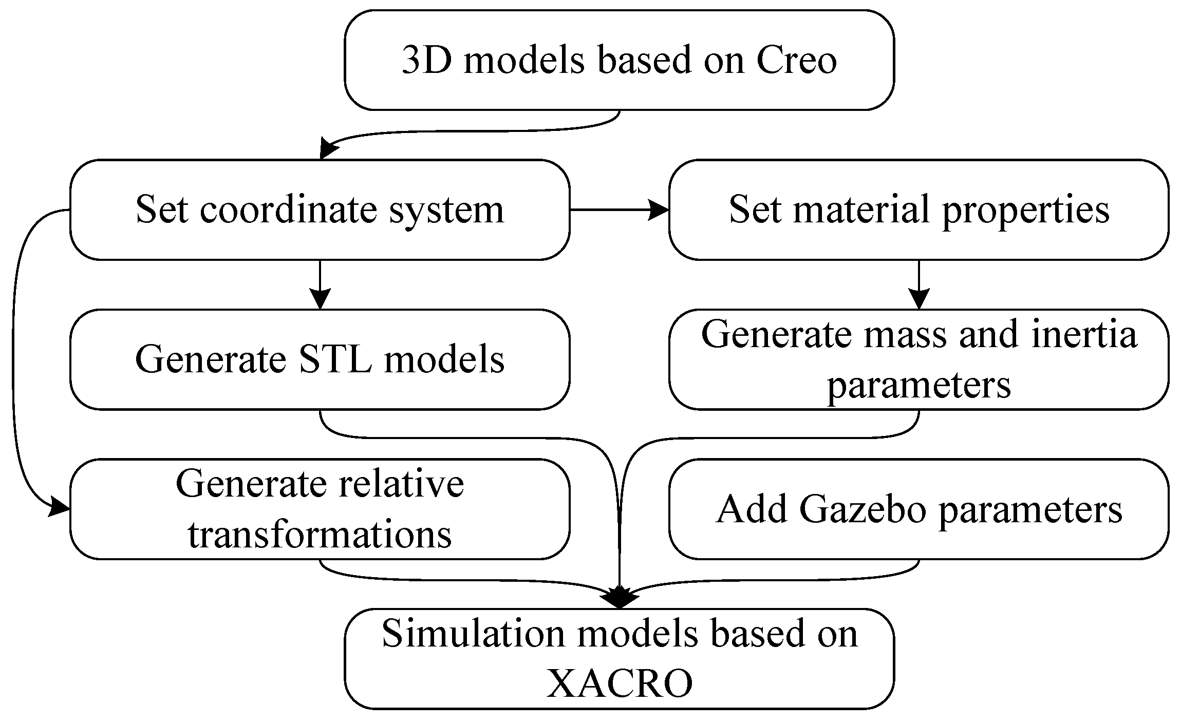
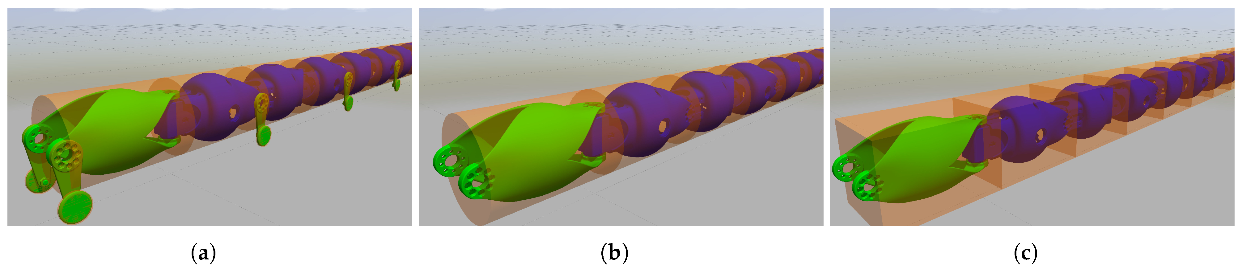
4.2. Simulator Module

To simulate snake robots and avoid some limitations in prototype experiments such as structural or performance indicators, we use Gazebo to establish a simulator module for snake robots. Gazebo supports various formats of robot models, such as the common unified robot description format (URDF), simulation description format (SDF), and XACRO. XACRO is a macro language based on the URDF, supports the description of the physical properties of objects and collision models, and can define repeated structures through macros. The snake robot consists of joint modules with the same simple structure from head to tail. Therefore, using XACRO to define snake robots can easily change the number of joints and parameters without re-modeling, achieving modularity and the parameterization of simulation models.

We designed three joint models for snake robots with different structures and sizes through Creo: Snake Robot I, Snake Robot II, and Snake Robot III. The orthogonal joint structures are shown in Figure 7, and the design parameters are shown in

Table 2. Design parameters of different snake robots.

Snake Robot	I	II	III
Length of linkage (m)	$0.076$	$0.106$	$0.160$
Number of joints	28	28	28
Range of joint (°)	±120	±90	±90
Passive wheel	Yes/No	Yes/No	Yes/No
Cross-section	Rectangle	Rectangle	Circle

. Each type of snake robot model corresponds to two situations: with and without passive wheels. The steps from the 3D model to the XACRO model are shown in Figure 8. We set the coordinate system and material properties in Creo and then export STL models, transformations among coordinate systems, and the inertia tensor parameters to establish the XACRO models for the snake robots. This paper establishes XACRO models for six types of snake robots, whereby three types with passive wheels are used for CL gait and the other three without passive wheels are used for complex three-dimensional motion gaits.

The motion simulation of the snake robots requires a lot of contact and collision calculation, which consumes many computing resources. To reduce the computational complexity and accelerate the simulation speed, we simplify the collision models for the snake robots, as shown in Figure 9. The joint structures are simplified into box or cylindrical models, and the simplified collision model can be applied to different gait movements. For example, the cylindrical collision model is used for SWL, ARL, and SRL, while the rectangular collision model can be used for TWL, SWL, and SRL. Gazebo controls the motion of each joint of the snake robot based on the desired joint position to achieve its motion simulation while simultaneously publishing joint and linkage states.

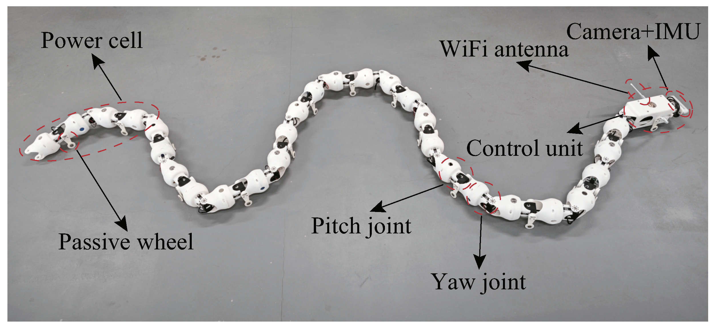
4.3. Prototype Module

To improve the load capacity and motion stability of the snake robots, we adopt an integrated design concept to complete the prototype of Snake Robot III. The orthogonal joint shape of the robot is close to a sphere, making it smoother during rolling and less likely to be stuck by obstacles. Each joint contains a specific cavity for installing components such as batteries, sensors, and control panels. The snake robot contains multiple orthogonal joint modules connected in sequence, so it can carry many batteries or sensors simultaneously, greatly improving its endurance capacity. The joint is 3D printed using white nylon material. Only four multifunctional joint shells are needed to assemble an orthogonal joint, which simplifies the structure of the prototype, reduces assembly time, and improves the structural stability of the snake robot.

To solve the power supply problem of motors, we designed a distributed power supply system for the snake robot, which is composed of multiple power cells, as shown in Figure 10. Each power cell consists of even motors and a rechargeable lithium battery, and the battery supplies power to these motors simultaneously. These motors are connected in series through power cables and signal buses in a power cell. A snake robot includes a control unit and multiple power cells in series and only a signal bus connection among them. This distributed power supply system can make the snake robot get rid of the power cord of the online power supply, realize flexible offline movement, and greatly improve its endurance.

The prototype of Snake Robot III is shown in Figure 11. The joint motor adopts the FEETECH SM8524BL DC serial bus digital servo to drive the joint motion directly. The control unit uses LattePanda 3 Delta as the prototype controller and collaborates with a notebook for large-scale computing task modules. The LattePanda 3 Delta has 8 GB RAM and 1 TB SSD. The notebook has an Intel i9-11980HK processor and an RTX3080 GPU, with 64 GB RAM and 16 GB of video memory, and they are configured with Ubuntu 20.04, ROS1 Noetic, and ROS2 Foxy. The sensor adopts Realsense D455 or ZED 2i, and they have an IMU and multiple cameras. The prototype utilizes a local area network (LAN) environment set up by a router to communicate with the notebook. The prototype is completely independent and does not have a signal bus or power cord connected to the outside; therefore, it can move freely within the coverage range of the LAN.

4.4. Perception Module

The prototype of Snake Robot III has visual and inertial sensors, and each joint motor has a magnetic encoder to provide the joint position. We integrate the ORB-SLAM3 system for SnakeSys, and it can generate the environment map and the left camera pose $T_{W,C_1}$ based on the image or IMU data collected during the motion of the snake robot [46]. The pose $T_{W,B}$ of the snake robot can be obtained based on the kinematic model in Section 2.3. The pose $T_{J_{i-1},J_i}$ of the joint linkage can be calculated based on the kinematic model in Section 2.2 and the joint-position feedback from the magnetic encoder. We build a $tf$$tree$ for the snake robot in the ROS for collision detection, motion planning, and autonomous navigation.

4.5. Motion-Control Module

To ensure that the CPG model generates a series of time-discrete joint-control sequences in real time at a specific frequency, we use the GNU Science Library (GSL) to construct the CPG module. Due to the GSL being written in C language, its computing speed is breakneck, and it can achieve robot-control frequencies from 10 Hz to 100 Hz under the condition of a communication baud rate of 1 Mbps for the joint motor of the snake robot.

4.6. High-Level-Control Module

The GUI module of the high-level-control module is based on Qt, which includes perception data visualization and parameter control, as shown in Figure 12. The data visualization can display feedback data from the sensors of the snake robot, such as the feedback joint position of each joint motor and the state of the coordinate system of the snake robot. The parameter control can change the robot-control frequency, joint amplitude, and joint frequency. In addition, the Logitech handle module is used to control the snake robot remotely. We also construct RViz configurations for SnakeSys to visualize the snake robot data. Visualizing data through RViz of the ROS is more convenient, but Qt-based GUI can add custom control logic and algorithms, complex interface layouts, and control components at the underlying level.

5. Simulations and Experiments

To verify the effectiveness and accuracy of the kinematic model, control model, and SnakeSys in simulating, controlling, and perceiving, we conduct simulation and experimental verifications on different motion gaits based on the simulation model and the prototype of Snake Robot III, and then compare and analyze the results.

5.1. Simulations for Multiple Motion Gaits in a Simple Environment

Due to the coupling gain coefficient $\alpha$ and attraction factor $\lambda$ affecting the synchronization speed and waveform change rate of the CPG model, we set $\alpha =0.01$ and $\lambda =0.2$ through empirical methods to ensure that the CPG model has a good synchronization speed and smooth waveform change state. The bifurcation parameter affects the convergence state of the oscillator, and setting ${\sigma }_1={\sigma }_2=\cdots ={\sigma }_N=1$ ensures that the amplitude parameter of the oscillator is consistent with the waveform amplitude. The simulation parameters corresponding to five motion gaits are shown in

Table 3. Parameter settings of different motion gaits in simulations.

Parameter	CL	TWL	SWL	ARL	SRL
$K_n$	2	3	2	−	−
$a_y$ (°)	50	$0.1$	50	−	−
$a_p$ (°)	$0.1$	50	15	−	−
$r_a$	−	−	−	2	−
$r_s$	−	−	−	−	$0.26$
$p_s$	−	−	−	−	$0.04$
$\omega$ ($\mathrm{rad}/\mathrm{s}$)	$\pi /5$	$-\pi /5$	$\pi /5$	$-\pi /2$	$\pi /5$

. Among them, the sign of the frequency $\omega$ only affects the direction of movement. For example, for TWL gait, negative frequency makes the snake robot move forward, while positive frequency makes it move backward. The cylinder collision model is used for CL, SWL, and ARL gaits, while the box collision model is used for TWL and SRL gaits. Using SnakeSys for simulation, the results are shown in Figure 13. The histograms of motion velocity and maximum joint torque corresponding to the five gaits are shown in Figure 14. To avoid the influence of $\omega$ on motion velocity, the velocity value in Figure 14a is equal to the velocity at $\omega =1\mathrm{rad}/\mathrm{s}$.

By comparing the variation in the joint position within a single period, as shown in Figure 13b,e,h,k,n, it can be found that the ARL gait has the smallest joint-motion amplitude, while both the TWL and SRL gaits have the largest joint-motion amplitude. This indicates that snake robots require specific joint-motion ranges to achieve different motion gaits. According to Figure 14b, as well as Figure 13c,f,i,l,o, the CL gait has the smallest torque while the SRL gait has the largest, almost 300 times that of the CL gait. The joint torque of the TWL and SWL gait are relatively close. According to Figure 14a, the CL gait has the highest motion velocity and the lowest joint torque, so it has the highest motion efficiency. The SRL gait has the highest joint torque, and it has the lowest efficiency. Therefore, the snake robot should prioritize using the CL gait. Although different motion gaits have different motion efficiencies, there is no superiority or inferiority in gaits, and the gait with lower motion efficiency may be needed to achieve obstacle avoidance and crossing.

5.2. Experiments for Multiple Motion Gaits in a Simple Environment

To verify the effectiveness of controlling the prototype and the accuracy of the simulator module of SnakeSys, we conduct experiments on the prototype of Snake Robot III. We deploy the servo motor-control node and frame-calculation node on the LattePanda 3 Delta and deploy the CPG control node and GUI node on the notebook. Due to the circle cross-section of Snake Robot III shown in Table 2 and Figure 7, the prototype is not suitable for achieving the TWL gait. According to the simulation torque of the SRL gait in Figure 14b, the joint torque exceeds the peak torque of the prototype motor. Therefore, we conduct experiments for the CL, SWL, and ARL gaits. The main control parameters for different motion gaits of the prototype are shown in

Table 4. Parameter settings of different motion gaits in experiments.

Parameter	CL	SWL	ARL
$K_n$	2	2	−
$a_y$ (°)	50	50	−
$a_p$ (°)	0.1	15	−
$r_a$	−	−	1
$\omega$ ($\mathrm{rad}/\mathrm{s}$)	$\pi /5$	$-\pi /5$	$\pi /2$

, and the other parameters are the same as in Section 5.1. The motion state, feedback joint position, desired joint position, and joint torque of the snake robot under different motion gaits are shown in Figure 15, according to which, based on the motion displacement and motion time of the snake robot under three different gaits, the motion velocities are obtained as 0.2553 m/s, 0.1415 m/s, and 0.0437 m/s, respectively, with frequency $\omega =1\mathrm{rad}/\mathrm{s}$.

Due to the inconsistency between the physical parameters involved in the experiment and those in the simulation, such as the ground friction coefficient, joint damping, joint linkage moment of inertia, etc., this paper uses the velocity ratio to compare the experimental and simulation results. The velocity ratio represents the ratio of the motion velocity of each gait to the CL gait. The velocity ratios of the experiment and simulation are shown in Figure 16, which indicates a high degree of consistency between the simulation and experimental results. According to Figure 15b,e,h, the actual variation pattern of the joint position of the snake robot is consistent with that of the desired joint position generated from the CPG model. The actual joint position lags behind the desired joint position in time because the desired joint position is given first and then each joint motor moves according to its value, and the joint motion of the snake robot macroscopically follows the fluctuation rhythm of the CPG output in real time. According to Figure 15c,f,i, the joint torque of experiments is consistent with simulations.

The above results indicate that the multimodal gait-control model in this paper can effectively control the different motion gaits of the snake robot in real time via both simulations and prototypes, and the simulator and simplified collision models in this paper have high consistency with the actual motion of the snake robot.

5.3. Experiments for Multiple Motion Gaits in Complex Environments

To verify the adaptability and maneuverability of the snake robot in complex environments, we conduct SWL and ARL experiments on grasses and rocks, respectively. The main experimental control parameters are shown in

Table 5. Parameter settings of control parameters in different environments.

Parameter	SWL1	SWL2	SWL3	SWL4	ARL1	ARL2	ARL3	ARL4
$K_n$	2	2	2	2	−	−	−	−
$a_y$ (°)	50	70	50	70	−	−	−	−
$a_p$ (°)	20	20	20	20	−	−	−	−
$r_a$	−	−	−	−	1	$1.2$	1	$1.2$
$\omega$ ($\mathrm{rad}/\mathrm{s}$)	$\pi /5$	$\pi /5$	$-\pi /5$	$-\pi /5$	$\pi /2$	$\pi /2$	$\pi /2$	$\pi /2$

, and other parameters are the same as in Section 5.1. The motion state, feedback joint position, desired joint position, and joint torque of the snake robot under different motion environments and gaits are shown in Figure 17. Based on the motion distance and joint torque, the corresponding motion velocity and maximum joint torque are calculated and shown in Figure 18.

According to Figure 17, the snake robot can maintain stable and continuous motion in complex environments, with strong environmental adaptability and traversability. Comparing Figure 15 and Figure 17, the motion direction of the snake robot in complex environments is easily affected by obstacles and contact conditions with the ground, and the ARL of the snake robot on rocks has better directional motion. According to Figure 18a, under the same oscillator frequency, the velocity of SWL is higher than that of ARL overall. However, under the same oscillator frequency and control parameters, the velocities of SWL are higher on grasses than on rocks, i.e., SWL1 > SWL3 and SWL2 > SWL4, and the velocities of ARL are higher on rocks than on grasses, i.e., ARL3 > ARL1 and ARL4 > ARL2. According to Figure 18b, the joint torque of SWL is generally greater than ARL, which is mainly related to the motion gait. The SWL gait requires lifting some joints off the ground and increasing the joint torque, while the ARL gait makes the body flat on the ground and the joint torque is relatively small.

Without a loss of generality, the ARL gait has a smaller joint torque and better motion directionality in complex environments, while the SWL gait has higher motion velocity but a larger joint torque. The passive wheel structure required for the CL gait is easily affected by obstacles, making the CL gait suitable for efficient movement on flat ground.

5.4. Information Perception of the Snake Robot

To verify the accuracy of the kinematic model established in this paper and the effectiveness of SnakeSys in snake robot perception, we conducted experiments on the environment mapping and localization of the snake robot using the Stereo algorithm of ORB-SLAM3. The image data are obtained from ZED 2i fixed on the head of the snake robot, with an image resolution of $1280\times 720$. At the same time, based on the joint-position feedback from the snake robot, its body shape in the CL gait was obtained using the kinematic model. The experimental results are shown in Figure 19, where Figure 19a shows the point cloud map of the environment and pose trajectory of the snake robot, and Figure 19b shows the body shape of the snake robot in RViz.

According to Figure 19, the environmental map and pose of the snake robot are consistent with the actual situation. The motion trajectory of the snake robot is an S-shaped curve, which is consistent with the CL gait of the snake robot. It should be pointed out that due to the perspective of the snake robot swinging left and right, especially when the initial angle of the waveform is large, its swing amplitude is also larger, so tracking loss is prone to occur during the SLAM operation. At the same time, we found during the experiment that there is a slight difference between the body shape of the snake robot obtained based on the assumption of joint linkage rigidity and the actual body shape, and the joint linkage of the snake robot will undergo slight deformation during motion.

6. Conclusions

In this paper, we established a coordinate system and kinematic model for a snake robot based on the D-H method; solved the perception of the body shape and pose in the environment during motion; and provided a theoretical basis for collision detection, motion planning, and autonomous navigation. Then, by introducing a bio-inspired CPG control model, the rhythm generation of different motion gaits of the snake robot was achieved, and a novel sliding-window five-point interpolation-derivative model was proposed to solve the generation of the joint velocity and acceleration for the CPG model, which improved the motion ability and environmental adaptability of the snake robot. In addition, three orthogonal joint modules and corresponding snake robots were designed, and a simulator for the snake robot based on Gazebo was established. A prototype of the snake robot with offline control, remote communication, and rich sensors was designed based on Snake Robot III and improved its motion flexibility and perception ability. Furthermore, an open-source SnakeSys for structure–drive–perception–control integration based on ROS2 and ROS1 was built, achieving multimodal motion control and information perception for snake robots. Finally, through simulations and experiments, the effectiveness and accuracy of SnakeSys in motion control and information perception of the snake robot were verified, providing a foundation for research on the motion control, motion planning, and autonomous navigation of snake robots.

In the subsequent research, we will focus on the state estimation of snake robots, considering the state estimation of snake robots with nonrigid joints and contact with the environment. To facilitate scholars or developers using SnakeSys for research on snake robots directly or further development on this basis, we open sourced SnakeSys. In addition to immediate issues and obstacles, the trajectory planning and control of SnakeSys require additional implementation and development.

References

1. Thandiackal, R.; Melo, K.; Paez, L.; Herault, J.; Kano, T.; Akiyama, K.; Boyer, F.; Ryczko, D.; Ishiguro, A.; Ijspeert, A.J. Emergence of robust self-organized undulatory swimming based on local hydrodynamic force sensing. Sci. Robot. 2021, 6, eabf6354. [Google Scholar] [CrossRef] [PubMed]
2. Liu, X.; Gao, Z.; Zang, Y.; Zhang, L. Tribological mechanism and propulsion conditions for creeping locomotion of the snake-like robot. J. Mech. Eng. 2021, 57, 13. [Google Scholar]
3. Megalingam, R.K.; Senthil, A.P.; Raghavan, D.; Manoharan, S.K. Modeling of novel circular gait motion through daisy sequence fitting algorithm in a vertical climbing snake robot. J. Field Robot. 2024, 41, 211–226. [Google Scholar] [CrossRef]
4. Ha, J. Robotic Snake Locomotion Exploiting Body Compliance and Uniform Body Tensions. IEEE Trans. Robot. 2023, 39, 3875–3887. [Google Scholar] [CrossRef]
5. Chang, A.H.; Vela, P.A. Shape-centric modeling for control of traveling wave rectilinear locomotion on snake-like robots. Robot. Auton. Syst. 2020, 124, 103406. [Google Scholar] [CrossRef]
6. Wang, T.; Lin, B.; Chong, B.; Whitman, J.; Travers, M.; Goldman, D.I.; Blekherman, G.; Choset, H. Reconstruction of backbone curves for snake robots. IEEE Robot. Autom. Lett. 2021, 6, 3264–3270. [Google Scholar] [CrossRef]
7. Arachchige, D.D.; Perera, D.M.; Mallikarachchi, S.; Kanj, I.; Chen, Y.; Godage, I.S. Wheelless soft robotic snake locomotion: Study on sidewinding and helical rolling gaits. In Proceedings of the 2023 IEEE International Conference on Soft Robotics (RoboSoft), Singapore, 3–7 April 2023; IEEE: Piscataway, NJ, USA, 2023; pp. 1–6. [Google Scholar]
8. Takemori, T.; Tanaka, M.; Matsuno, F. Adaptive helical rolling of a snake robot to a straight pipe with irregular cross-sectional shape. IEEE Trans. Robot. 2022, 39, 437–451. [Google Scholar] [CrossRef]
9. Liu, Y. Review of snake robots in constrained environments. Robot. Auton. Syst. 2021, 141, 103785. [Google Scholar] [CrossRef]
10. Wang, G.; Yang, W.; Shen, Y.; Shao, H.; Wang, C. Adaptive path following of underactuated snake robot on unknown and varied frictions ground: Theory and validations. IEEE Robot. Autom. Lett. 2018, 3, 4273–4280. [Google Scholar] [CrossRef]
11. Mori, M.; Hirose, S. Three-dimensional serpentine motion and lateral rolling by active cord mechanism ACM-R3. In Proceedings of the Intelligent Robots and Systems, 2002. IEEE/RSJ International Conference, Lausanne, Switzerland, 30 September–4 October 2002. [Google Scholar]
12. Komura, H.; Yamada, H.; Hirose, S. Development of snake-like robot ACM-R8 with large and mono-tread wheel. Adv. Robot. 2015, 29, 1081–1094. [Google Scholar] [CrossRef]
13. Ohno, H.; Hirose, S. Pneumatically-Driven Active Cord Mechanism “Slim Slime Robot”. J. Robot. Mechatron. 2014, 26, 105–106. [Google Scholar] [CrossRef]
14. Zuo, X.; Tang, J.; Tian, M.; Wang, X. A design of a snake robot inspired by waterbomb origami. In Proceedings of the 2022 IEEE International Conference on Robotics and Biomimetics (ROBIO), Jinghong, China, 5–9 December 2022; IEEE: Piscataway, NJ, USA, 2022; pp. 2354–2360. [Google Scholar]
15. Bi, Z.; Xu, J.; Fang, H. Design and path planning for a Worm-Snake-Inspired Metameric (WSIM) Robot. In Proceedings of the 2022 IEEE International Conference on Robotics and Biomimetics (ROBIO), Jinghong, China, 5–9 December 2022; IEEE: Piscataway, NJ, USA, 2022; pp. 777–782. [Google Scholar]
16. Qi, X.; Shi, H.; Pinto, T.; Tan, X. A novel pneumatic soft snake robot using traveling-wave locomotion in constrained environments. IEEE Robot. Autom. Lett. 2020, 5, 1610–1617. [Google Scholar] [CrossRef]
17. Gautreau, E.; Sandoval, J.; Bonnet, X.; Arsicault, M.; Zeghloul, S.; Laribi, M.A. A new bio-inspired Hybrid Cable-Driven Robot (HCDR) to design more realistic snakebots. In Proceedings of the 2022 International Conference on Robotics and Automation (ICRA), Philadelphia, PA, USA, 23–27 May 2022; IEEE: Piscataway, NJ, USA, 2022; pp. 2134–2140. [Google Scholar]
18. Hirose, S.; Yamada, H. Snake-like robots [tutorial]. IEEE Robot. Autom. Mag. 2009, 16, 88–98. [Google Scholar] [CrossRef]
19. Ma, S. Analysis of snake movement forms for realization of snake-like robots. In Proceedings of the 1999 IEEE International Conference on Robotics and Automation (Cat. No. 99CH36288C), Detroit, MI, USA, 10–15 May 1999; IEEE: Piscataway, NJ, USA, 1999; Volume 4, pp. 3007–3013. [Google Scholar]
20. Tang, C.; Sun, L.; Zhou, G.; Shu, X.; Tang, H.; Wu, H. Gait Generation Method of Snake Robot Based on Main Characteristic Curve Fitting. Biomimetics 2023, 8, 105. [Google Scholar] [CrossRef]
21. Takemori, T.; Tanaka, M.; Matsuno, F. Hoop-Passing Motion for a Snake Robot to Realize Motion Transition across Different Environments. IEEE Trans. Robot. 2021, 37, 1696–1711. [Google Scholar] [CrossRef]
22. Yu, J.; Tan, M.; Chen, J.; Zhang, J. A Survey on CPG-Inspired Control Models and System Implementation. IEEE Trans. Neural Netw. Learn. Syst. 2017, 25, 441–456. [Google Scholar] [CrossRef]
23. Ijspeert, A.J. Central pattern generators for locomotion control in animals and robots: A review. Neural Netw. 2008, 21, 642–653. [Google Scholar] [CrossRef] [PubMed]
24. Lin, F.; Zhang, G. Multimodal swimming control of bionic fish based on CPG. In Proceedings of the 2023 35th Chinese Control and Decision Conference (CCDC), Yichang, China, 20–22 May 2023; IEEE: Piscataway, NJ, USA, 2023; pp. 4633–4638. [Google Scholar]
25. Shaw, S.; Sartoretti, G. Keyframe-based CPG for stable gait design and online transitions in legged robots. In Proceedings of the 2022 IEEE 61st Conference on Decision and Control (CDC), Cancun, Mexico, 6–9 December 2022; IEEE: Piscataway, NJ, USA, 2022; pp. 756–763. [Google Scholar]
26. Song, Z.; Huang, X.; Xu, J. Spatiotemporal pattern of periodic rhythms in delayed Van der Pol oscillators for the CPG-based locomotion of snake-like robot. Nonlinear Dyn. 2022, 110, 3377–3393. [Google Scholar] [CrossRef]
27. Song, Z.; Xu, J. Multi-coexistence of routes to chaos in a delayed half-center oscillator (DHCO) system. Nonlinear Dyn. 2024, 112, 1469–1486. [Google Scholar] [CrossRef]
28. Song, Z.; Xu, J. Multiple switching and bifurcations of in-phase and anti-phase periodic orbits to chaotic coexistence in a delayed half-center CPG oscillator. Nonlinear Dyn. 2023, 111, 16569–16584. [Google Scholar] [CrossRef]
29. Song, Z.; Xu, J. Self-/mutual-symmetric rhythms and their coexistence in a delayed half-center oscillator of the CPG neural system. Nonlinear Dyn. 2022, 108, 2595–2609. [Google Scholar] [CrossRef]
30. Yang, G.; Ma, S.; Li, B.; Wang, M. A hierarchical connectionist CPG controller for controlling the snake-like robot’s 3-dimensional gaits. In Proceedings of the 2012 IEEE/RSJ International Conference on Intelligent Robots and Systems, Vilamoura-Algarve, Portugal, 7–12 October 2012; IEEE: Piscataway, NJ, USA, 2012; pp. 822–827. [Google Scholar]
31. Manzoor, S.; Choi, Y. A unified neural oscillator model for various rhythmic locomotions of snake-like robot. Neurocomputing 2016, 173, 1112–1123. [Google Scholar] [CrossRef]
32. Zhang, D.; Xiao, Q.; Cao, Z. Gait Generation with Smooth Transition Using Neural Oscillator Network Based Locomotion Control for Snake-Like Robot. In Proceedings of the 2019 2nd IEEE International Conference on Soft Robotics (RoboSoft), Seoul, Republic of Korea, 14–18 April 2019. [Google Scholar]
33. Wang, Z.; Gao, Q.; Zhao, H. CPG-Inspired Locomotion Control for a Snake Robot Basing on Nonlinear Oscillators. J. Intell. Robot. Syst. 2017, 85, 209–227. [Google Scholar] [CrossRef]
34. Fukuoka, Y.; Otaka, K.; Takeuchi, R.; Shigemori, K.; Inoue, K. Mechanical Designs for Field Undulatory Locomotion by a Wheeled Snake-Like Robot with Decoupled Neural Oscillators. IEEE Trans. Robot. 2023, 39, 959–977. [Google Scholar] [CrossRef]
35. Burden, S.A.; Libby, T.; Jayaram, K.; Sponberg, S.; Donelan, J.M. Why animals can outrun robots. Sci. Robot. 2024, 9, eadi9754. [Google Scholar] [CrossRef]
36. Macenski, S.; Soragna, A.; Carroll, M.; Ge, Z. Impact of ROS 2 Node Composition in Robotic Systems. IEEE Robot. Autom. Lett. 2023. [Google Scholar] [CrossRef]
37. Macenski, S.; Foote, T.; Gerkey, B.; Lalancette, C.; Woodall, W. Robot Operating System 2: Design, architecture, and uses in the wild. Sci. Robot. 2022, 7, eabm6074. [Google Scholar] [CrossRef]
38. Koenig, N.; Howard, A. Design and use paradigms for gazebo, an open-source multi-robot simulator. In Proceedings of the 2004 IEEE/RSJ International Conference on Intelligent Robots and Systems (IROS) (IEEE Cat. No. 04CH37566), Sendai, Japan, 28 September–2 October 2004; IEEE: Piscataway, NJ, USA, 2004; Volume 3, pp. 2149–2154. [Google Scholar]
39. Sanfilippo, F.; Stavdahl, Ø.; Liljebäck, P. SnakeSIM: A ROS-based rapid-prototyping framework for perception-driven obstacle-aided locomotion of snake robots. In Proceedings of the 2017 IEEE International Conference on Robotics and Biomimetics (ROBIO), Macau, China, 5–8 December 2017; IEEE: Piscataway, NJ, USA, 2017; pp. 1226–1231. [Google Scholar]
40. Ni, F.; Li, Y.; Zhou, Y.; Zhao, L.; Liu, H. Design of a Hierarchical Control System for Tetherless Snake Robot. In Proceedings of the 2019 IEEE International Conference on Mechatronics and Automation (ICMA), Tianjin, China, 4–7 August 2019; IEEE: Piscataway, NJ, USA, 2019; pp. 1254–1259. [Google Scholar]
41. Zhou, Y.; Li, Z.; Zhang, Y.; Ni, F.; Sun, Y.; Liu, H. The real-time control framework for a modular snake robot. In Proceedings of the 2019 4th International Conference on Robotics and Automation Engineering (ICRAE), Singapore, 22–24 November 2019; IEEE: Piscataway, NJ, USA, 2019; pp. 168–172. [Google Scholar]
42. Ding, C.; Zhou, J.; Wu, L.; Ren, C. Path Planning and Gait Control of Snake Robot Based on PAPF and MPC. In Proceedings of the 2023 42nd Chinese Control Conference (CCC), Tianjin, China, 24–26 July 2023; IEEE: Piscataway, NJ, USA, 2023; pp. 2934–2939. [Google Scholar]
43. Melo, K.; Leon, J.; di Zeo, A.; Rueda, V.; Roa, D.; Parraga, M.; Gonzalez, D.; Paez, L. The modular snake robot open project: Turning animal functions into engineering tools. In Proceedings of the 2013 IEEE International Symposium on Safety, Security, and Rescue Robotics (SSRR), Linköping, Sweden, 21–26 October 2013; IEEE: Piscataway, NJ, USA, 2013; pp. 1–6. [Google Scholar]
44. Cai, Z. Fundamentals of Robotics; China Machine Press: Beijing, China, 2021. [Google Scholar]
45. Liu, X.; Zang, Y.; Gao, Z.; Liao, M. Locomotion gait control of snake robots based on a novel unified CPG network model composed of Hopf oscillators. Robot. Auton. Syst. 2024, 179, 104746. [Google Scholar] [CrossRef]
46. Campos, C.; Elvira, R.; Rodríguez, J.J.G.; Montiel, J.M.; Tardós, J.D. ORB-SLAM3: An accurate open-source library for visual, visual–inertial, and multimap slam. IEEE Trans. Robot. 2021, 37, 1874–1890. [Google Scholar] [CrossRef]
Figure 1. Coordinate system of the snake robot.
Electronics 13 03437 g001
Figure 2. Rotating pair and linkage parameters of joints of the snake robot.
Electronics 13 03437 g002
Figure 3. Bio -inspired CPG control based on Hopf oscillators of the snake robot.
Electronics 13 03437 g003
Figure 4. Five-point interpolation-derivative model based on sliding window for CPG model. S1 and S4 represent that they are not fixed after calculation using Equations (40) and (45), respectively. S2 represents that they are not fixed after calculation using Equation (39). S3 and S5 represent that they are fixed after calculation using Equations (38) and (43), respectively.
Electronics 13 03437 g004
Figure 5. Control architecture of SnakeSys.
Electronics 13 03437 g005
Figure 6. Nodes and topics of SnakeSys.
Electronics 13 03437 g006
Figure 7. Orthogonal joints corresponding to Snake Robot I, Snake Robot II, and Snake Robot III.
Electronics 13 03437 g007
Figure 8. Steps from the Creo model to the XACRO model.
Electronics 13 03437 g008
Figure 9. The simplified collision models for Snake Robot III. (a) Cylinder collision model with passive wheels. (b) Cylinder collision model without passive wheels. (c) Box collision model without passive wheels.
Electronics 13 03437 g009
Figure 10. The distributed power supply system for snake robots.
Electronics 13 03437 g010
Figure 11. Prototype of Snake Robot III.
Electronics 13 03437 g011
Figure 12. The GUI module of SnakeSys. (a) Parameter control of the GUI module. (b) Data visualization of the GUI module. (c) The state of the snake robot in Gazebo. (d) Visualization of t f t r e e in RViz.
Electronics 13 03437 g012
Figure 13. The motion of the snake robot in CL, TWL, SWL, ARL, and SRL gaits. The green curve from light to deep represents the yaw joints numbered from small to large and the purple curve from light to deep represents the pitch joints numbered from small to large.
Electronics 13 03437 g013aElectronics 13 03437 g013b
Figure 14. The movement velocity and maximum joint torque of five gaits.
Electronics 13 03437 g014
Figure 15. The motion of the snake robot in CL, SWL, and ARL gaits. The green curve from light to deep represents the yaw joints numbered from small to large and the purple curve from light to deep represents the pitch joints numbered from small to large. The dashed line represents the desired joint position generated from the CPG model.
Electronics 13 03437 g015
Figure 16. The motion velocity ratio of experiments and simulations.
Electronics 13 03437 g016
Figure 17. The motion of the snake robot in different environments. The green curve from light to deep represents the yaw joints numbered from small to large, and the purple curve from light to deep represents the pitch joints numbered from small to large. The dashed line represents the desired joint position generated from the CPG model.
Electronics 13 03437 g017aElectronics 13 03437 g017b
Figure 18. The movement velocity and maximum joint torque in different environments.
Electronics 13 03437 g018
Figure 19. Information perception of the snake robot under CL gait. (a) Point cloud map and pose trajectory of the snake robot. (b) The body shape and tracking point cloud of the snake robot.
Electronics 13 03437 g019