A Multidimensional Framework Incorporating 2D U-Net and 3D Attention U-Net for the Segmentation of Organs from 3D Fluorodeoxyglucose-Positron Emission Tomography Images

Abstract

Accurate analysis of Fluorodeoxyglucose (FDG)-Positron Emission Tomography (PET) images is crucial for the diagnosis, treatment assessment, and monitoring of patients suffering from various cancer types. FDG-PET images provide valuable insights by revealing regions where FDG, a glucose analog, accumulates within the body. While regions of high FDG uptake include suspicious tumor lesions, FDG also accumulates in non-tumor-specific regions and organs. Identifying these regions is crucial for excluding them from certain measurements, or calculating useful parameters, for example, the mean standardized uptake value (SUV) to assess the metabolic activity of the liver. Manual organ delineation from FDG-PET by clinicians demands significant effort and time, which is often not feasible in real clinical workflows with high patient loads. For this reason, this study focuses on automatically identifying key organs with high FDG uptake, namely the brain, left cardiac ventricle, kidneys, liver, and bladder. To this end, an ensemble approach is adopted, where a three-dimensional Attention U-Net (3D AU-Net) is employed for robust three-dimensional analysis, while a two-dimensional U-Net (2D U-Net) is utilized for analysis in the coronal plane. The 3D AU-Net demonstrates highly detailed organ segmentations, but also includes many false positive regions. In contrast, 2D U-Net achieves higher reliability with minimal false positive regions, but lacks the 3D details. Experiments conducted on a subset of the public AutoPET dataset with 60 PET scans demonstrate that the proposed ensemble model achieves high accuracy in segmenting the required organs, surpassing current state-of-the-art techniques, and supporting the potential utilization of the proposed methodology in accelerating and enhancing the clinical workflow of cancer patients.

1. Introduction

Medical imaging plays a vital role in the diagnosis, treatment planning, and monitoring of various diseases. Among the different imaging modalities available, Fluorodeoxyglucose-Positron Emission Tomography (FDG-PET) has emerged as a powerful tool in oncology and neurology due to its ability to provide functional information about metabolic activity within tissues [1]. The accurate and automated segmentation of organs (allowing for the precise delineation and extraction of anatomical structures or regions of interest) from FDG-PET images is crucial for precise disease assessment, treatment response evaluation, and surgical planning [2]. However, in clinical practice, it is imperative that medical professionals have confidence in the tools they use, accurately measuring the size, volume, and growth rate of organs, tumors, and lesions [3]. Traditional manual segmentation methods are not only time consuming and labor intensive but also prone to variability between and within observers [4]. Consequently, there is an increasing demand for advanced computer-assisted techniques that can automate this process while maintaining high levels of accuracy and reproducibility. In this regard, machine learning has already made significant contributions to medicine and will continue to assist with various medical tasks, allowing for the earlier and more accurate detection of medical conditions [5,6]. Furthermore, advanced segmentation algorithms facilitate precise delineation of anatomical structures and pathological regions, reducing the likelihood of misdiagnosis and helping to ensure that subtle abnormalities are not overlooked [7]. In surgical planning, clear organ delineation helps surgeons plan procedures with greater confidence, reducing operative time, minimizing the risk of complications, and increasing the success rate of surgeries. When segmentation guides therapy, such as in radiotherapy or surgery, more precise targeting reduces the risk of damaging healthy tissue, leading to fewer side effects and better overall patient quality of life [8].

Semantic segmentation (the task of assigning a predefined class to each pixel) is central to these efforts, demanding a profound visual understanding to ensure precision and reliability in clinical outcomes. On this premise, semantic segmentation networks have evolved, with some of the most impactful architectures contributing to advancements in organ segmentation. For instance, SegNet, introduced by Vijay Badrinarayanan et al. [9], is an encoder–decoder network, which uses convolutional and pooling layers for down-sampling in the encoder and up-sampling in the decoder, laid the groundwork for subsequent developments in the field. In addition, architectures like U-Net, DeepLab, and SegResNet have emerged, offering enhanced performance for organ segmentation tasks [10,11,12]. Among these, U-Net has become particularly popular, featuring a characteristic “U” shape formed by its encoding contracting pathway and expansive decoding pathway [10]. The contracting pathway down-samples the input image through convolutional and pooling operations, while the expansive pathway upscales the feature maps using transposed convolutional layers. Skip connections between corresponding layers in the encoding and decoding pathways allow U-Net to recover spatial details effectively, leading to more accurate segmentation outcomes. Expanding upon the U-Net framework, nnU-Net can self-configure and adapt to any dataset, delivering high performance, enabling it to excel across various medical segmentation tasks [13]. Moreover, DeepLab has made notable contributions to semantic segmentation, particularly through the use of atrous (or dilated) convolutions [11]. This allows DeepLab models, including DeepLabv2, DeepLabv3, and DeepLabv3+, to capture multi-scale information effectively without significantly increasing computational costs [11,14,15]. Recently, the transformers can capture global context and long-range dependencies, a feature that traditional convolutional neural networks (CNNs) lack [16]. UNETR, a hybrid architecture combining U-Net and transformers, leverages this capability to address the limitations of conventional CNNs, offering enhanced segmentation accuracy [17].

Despite significant recent advancements in machine learning for medical imaging, segmenting organs from 3D FDG-PET images remains a challenge due to several inherent factors of diagnostic visualization. FDG-PET images are characterized by low spatial resolution, limited contrast, and substantial noise, all of which can impede the precise delineation of organ boundaries [18]. Additionally, variations in image intensity caused by differences in patient physiology, imaging protocols, and equipment settings further complicate the segmentation process. In our previous study focusing on the identification of Metastatic Melanoma tumors from FDG-PET/CT images, organs with high uptake in them produce many false positives when a model tries to locate tumor lesions throughout the body [19].

To overcome these obstacles, in this study, we propose a machine learning framework for organ segmentation in PET data through an ensemble model that effectively integrates 2D and 3D data perspectives. Our rationale stems from the fact that 2D and 3D networks (i.e., Attention U-Net (3D AU-Net) [20,21] and two-dimensional U-Net [10] (2D U-Net)) can enhance flexibility and improve performance (especially when 3D data is unreliable or computational resources are limited), harnessing slice-wise processing (2D U-Net) and the ability to capture spatial dependencies across slices (3D AU-Net’s). From this standpoint, the combined model can increase adaptability and may lead to better generalization across varied datasets or conditions. As such we aim to carry out the following:

• Address a significant gap in the field by providing a dedicated solution for segmenting PET images;
• Leverage the power of combined machine learning models to enhance automatic segmentation performance;
• Propose a new, ensemble approach, that is particularly suited for achieving high validation performance when training on limited samples.

In this regard, utilizing an annotated PET dataset of 60 scans, we combine the 3D AU-Net volumetric understanding with the 2D U-Net slice-wise processing capabilities to enhance specific clinical applications in PET image segmentation which are often overlooked in favor of other imaging modalities like CT or MRI. The proposed method results in a high segmentation performance regarding the brain, left cardiac ventricle, kidneys, liver, and bladder. Rigorous testing displays significant improvement in segmentation accuracy, outperforming benchmark models and the individual 2D U-Net and 3D AU-Net counterparts.

2. Materials and Methods

2.1. Dataset

In the proposed methodology, a subset of the public AutoPET [22] dataset with 60 PET scans was used, due to these volumes being the only ones to contain annotations for all target organs. The AutoPet dataset contains a total of 1,014 PET scans. Of these scans, 501 studies were from patients with malignant lymphoma, melanoma, and non-small cell lung cancer (NSCLC), and 513 studies without PET-positive malignant lesions (negative controls). All examinations were conducted at the University Hospital Tübingen using a single PET/CT scanner (Siemens Biograph mCT, Siemens Healthineers, Knoxville, TN, USA). Both CT and PET scans followed standardized protocols to ensure uniformity across all studies. Specifically, CT scans were performed with a consistent set of scan parameters, including slice thickness, tube voltage, and current, while PET scans adhered to a uniform acquisition time and reconstruction algorithm. The only variable was the dose of the F-FDG injection, which was adjusted based on the patient’s weight to optimize image quality. For this subset, experts created detailed masks for the following organs: bladder, brain, liver, left ventricle of the heart, and kidneys. The dataset offers 3D volumes of both CT and FDG PET data, presented as stacks of axial slices, and all the data covers comprehensive whole-body examinations. The usual scan range encompasses from the skull base to the mid-thigh level, with the potential for extension to include the entire body, head to legs, based on clinical necessity. The chosen scans consist of whole body FDG PET/CT images. The PET data were reconstructed iteratively with Gaussian post-reconstruction smoothing. Then, standardization was applied by converting image units from activity counts to standardized uptake values (SUV).

2.2. Ensemble Model Architecture

The neural network approach proposed in this study consists of an ensemble of two U-Net architectures that complement each other.

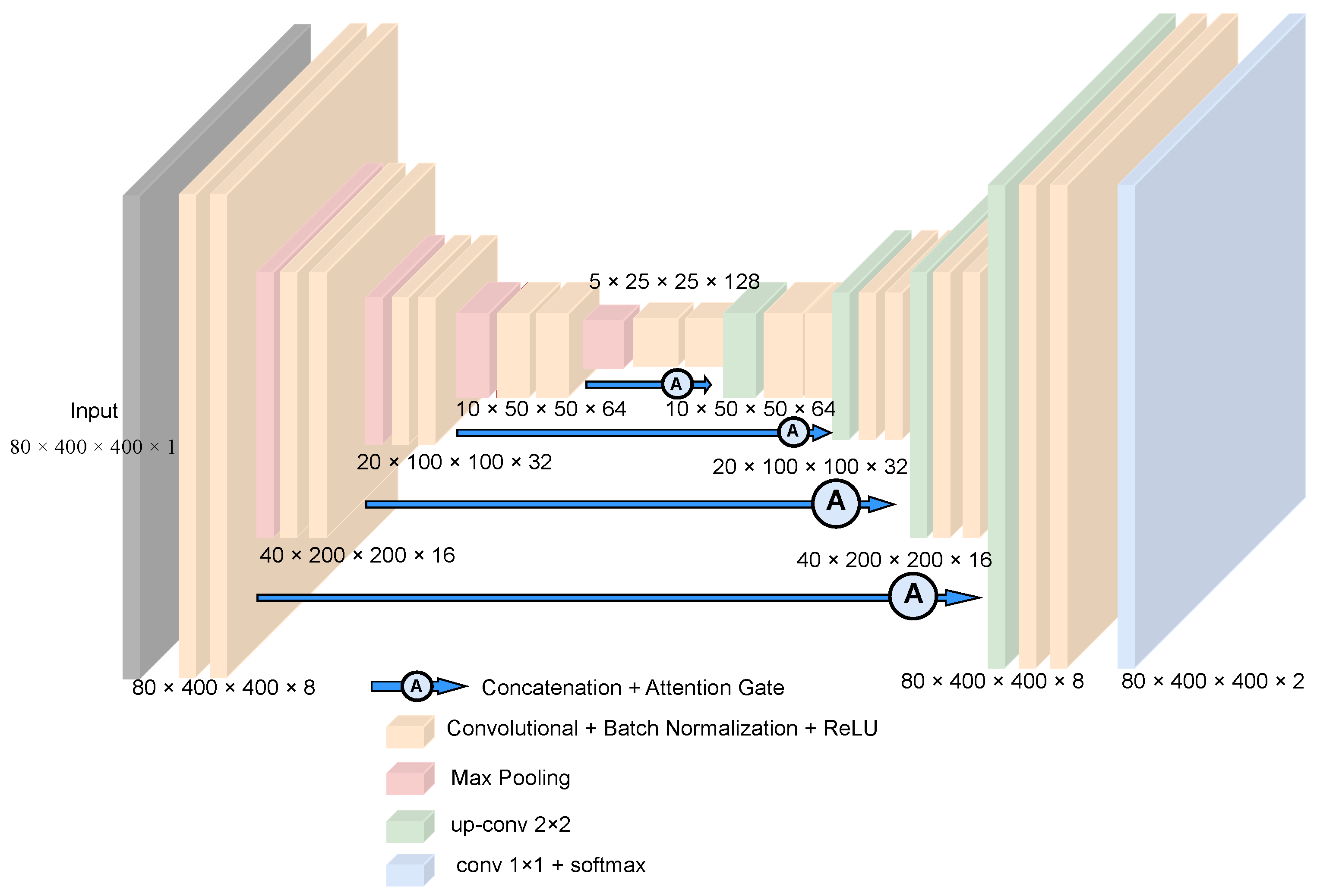
2.2.1. 3D AU-Net

The first U-Net utilized is a three-dimensional Attention U-Net for robust three-dimensional analysis. What sets this architecture apart is the use of Attention Gates, a mechanism that improves performance in tasks requiring precise localization by learning to selectively focus on particular regions of interest [20]. It takes feature maps from the encoder and decoder, computes attention maps to highlight important regions, and uses these maps to weight the feature maps from the encoder before merging them with the decoder’s feature maps. The most significant advantage of using a 3D architecture is its ability to leverage volumetric information. It considers spatial relationships in all three dimensions (X, Y, and Z), capturing contextual information from adjacent slices. This allows the model to better understand the 3D structure of objects and organs within the volume. The architecture of our three-dimensional Attention U-Net comprises four convolutional blocks in each of the encoding and decoding pathways, as depicted in Figure 1. The original volumes are of shape N × 400 × 400 × 1, where N is the depth dimension and varies between individuals. During training, each volume is divided into overlapping (along the depth dimension) patches of size 80 × 400 × 400 × 1, which are individually fed to the network and are gradually reduced to size 5 × 25 × 25 × 128, where 128 is the number of feature maps produced. In the decoding pathway, the patch volumes are gradually upscaled to 80 × 400 × 400 × 8 voxels. Subsequently, a 1 × 1 convolutional operation is applied, which is often referred to as a pointwise convolution. This operation serves to merge information from the different channels and generate the final output. Deep supervision [23] was added to the model for the computation of loss, a technique pivotal in enhancing the training process of neural networks. Deep supervision involves the incorporation of additional supervision signals at intermediate layers of the network architecture, thereby facilitating more effective gradient flow and addressing the issue of vanishing gradients. This approach fosters better convergence during training, enabling the network to learn more efficiently and yielding improved performance outcomes.

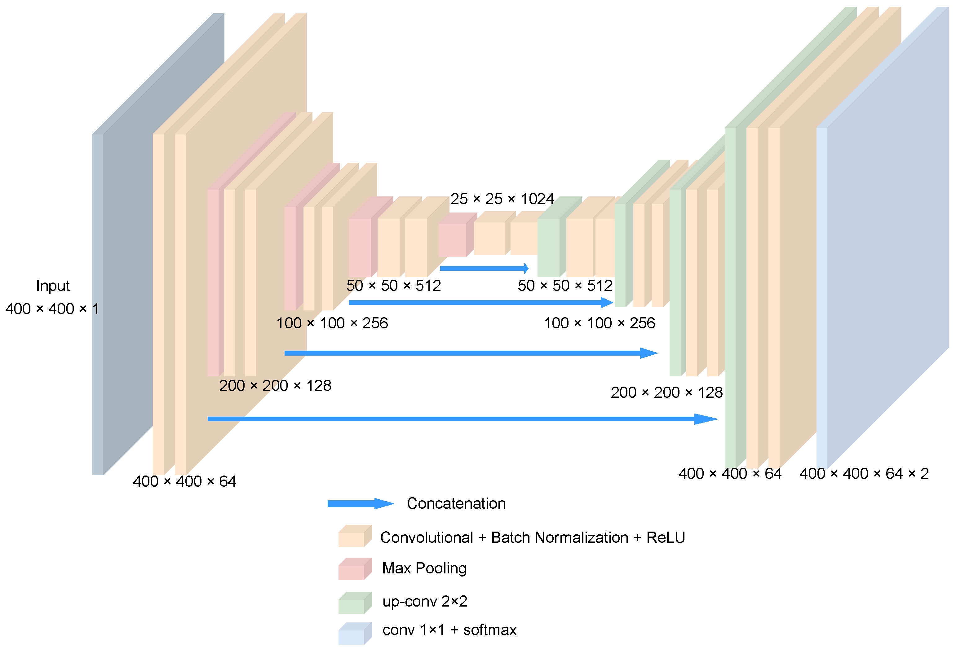
2.2.2. 2D U-Net

The second U-Net used in this study is a two-dimensional U-Net (2D U-Net). To facilitate this transition, the three-dimensional data were converted into two-dimensional coronal view images, as it was heuristically observed that the model exhibited superior recall performance in this orientation compared to sagittal and axial views. The input to this network is an image with dimensions 400 × 400 × 1 pixels. The architecture, like in the 3D variant, includes four convolutional blocks in each of the encoding and decoding pathways, as depicted in Figure 2. The encoding pathway progressively reduces the spatial dimensions to 25 × 25 × 1024, before being up-sampled back to its original size by the decoding pathway.

2.2.3. Ensemble

The final neural network model employed in this study is an ensemble of 2D U-Net and 3D AU-Net. Despite their architectural similarities, each model yields different end results and thus their combination enhances the overall final accuracy. The two models are trained independently. Upon completion of training for both networks, a straightforward post-processing procedure is applied.

Initially, the segmentation masks computed by 2D U-Net are combined into a unified 3D volume. Since 2D U-Net operates independently on individual slices, any false positive regions are likely to be isolated to specific slices. When the 2D segmentation masks are combined into a 3D volume, these isolated false positives do not align or connect with one another across slices. Since false positives tend to be random and scattered, their lack of spatial continuity means they remain small and isolated when viewed in the context of the entire 3D volume. In contrast, the true organ regions are more likely to be spatially continuous across multiple adjacent slices. When these consistent regions are combined into a 3D volume, they form a large, connected component, representing the actual structure of the organ. The largest connected component in the 3D mask is therefore likely to correspond to the true organ, while the false positives, being smaller and more fragmented, do not combine into significant structures. To isolate this true positive component, we apply a simple criterion of selecting the largest connected component within the mask.

Subsequently, the segmentation results of the patches from the 3D AU-Net are aggregated to generate a second segmentation mask for the entire volume. Since the 3D AU-Net processes patches of the 3D volume, and not the entire scan at once, each patch is segmented independently. For overlapping patches, their union is computed. However, because of the complexity and sensitivity of the model, this also introduces numerous false positives. To improve the accuracy of the segmentation, the outputs of both 2D U-Net and 3D AU-Net are combined. 2D U-Net provides a coarser but more reliable segmentation, giving a general idea of where the target organ is located. The 3D AU-Net, while more detailed, includes many false positives due to its finer resolution. Therefore, the final step involves selectively merging the outputs from 2D U-Net and 3D AU-Net. By focusing on the regions where the segmentations from both networks overlap, the method capitalizes on the strengths of each model: 2D U-Net’s robustness in avoiding false positives and 3D AU-Net’s detailed segmentation. The rationale is that the true organ region is likely to be consistently identified by both networks, resulting in an overlapping area that represents the most reliable segmentation. Figure 3 graphically depicts this process, visualizing the outputs masks of 2D U-Net, 3D AU-Net, and the ensemble method.

2.3. Training Setup

To ensure data consistency and improve training effectiveness through a uniform voxel spacing, all volumes were ensured to have the same uniform voxel spacing values of (2.036, 2.036, 3.0) prior to training, as computed by the median value. The voxel spacing values indicate the distance between the slices in the Z plane, and the distance between neighboring pixels in the X and Y plane. Voxel spacing normalization is crucial for medical imaging, as scans from different patients or scanners might have varying resolutions or slice thicknesses. It has previously been shown that voxel normalization is a crucial pre-processing step as it directly impacts performance in texture-related studies [24]. In addition, the uniformity achieved across all samples ensures that the models do not learn scanner- or patient-specific biases corresponding to different resolutions and scales [25].

In addition, intensity normalization was applied, centering the data around their mean and scaling them by their standard deviation, resulting in voxels with a mean intensity of 0 and a standard deviation of 1. This pre-processing step helps in stabilizing the gradients during backpropagation, which contributes to solving problems like vanishing or exploding gradients. Moreover, intensity normalization makes sure that all input features are on a similar scale, resulting in faster model convergence during training. Otherwise, the model needs to adjust its weights to accommodate the large differences in input scales, slowing down the training [26].

Regularization techniques are critical in neural networks to prevent overfitting and improve generalization to unseen data. Overfitting occurs when a model performs well on the training data but fails to generalize to new data. One widely used regularization method is Batch Normalization, which normalizes the inputs to each layer by adjusting and scaling activations. By stabilizing the learning process, Batch Normalization inherently acts as a form of regularization, potentially reducing the need for other techniques like Dropout [27]. We implemented this technique in all our experiments. Another regularization method used in our experiments is data augmentation. Data augmentation is a technique used to artificially expand the size of a training dataset by applying various transformations to the existing data. By introducing variations such as rotations, translations, flips, scaling, and adjustments in brightness or contrast, it enhances the model’s ability to generalize by exposing it to a wider variety of scenarios during training, and thereby reducing the risk of overfitting. In our training procedures, we applied random rotations of up to 20 degrees, horizontal and vertical flips with a 50% probability, scaling within a range of 0.8 to 1.2, and brightness adjustments varying by ±10%.

Each network was individually trained multiple times using varying amounts of data (15, 20, 30, 40, and 50 samples), with consistent validation across all experiments using a fixed set of 10 data points. This approach ensured robustness and reliability in our assessment, as it allowed us to observe the performance of each network under different training conditions and data quantities. The 3D AU-Net network was trained for a total of 50 epochs, and 2D U-Net for a total of 25 epochs, as further training was not found to further decrease training loss. To calculate the loss, the combined sum of the Dice score [28] and cross-entropy [29] loss was utilized. Dice score is a popular metric employed in numerous image segmentation tasks, including biomedical segmentation. The Dice loss focuses on measuring the spatial agreement between the predicted segmentation mask and the ground truth, making it particularly effective for dealing with imbalanced data. Mathematically, the Dice loss is calculated as follows:

$$\mathrm{Dice}\mathrm{Loss}=1-{\displaystyle \frac{2·\mathrm{Intersection}}{\mathrm{Union}+\mathrm{Intersection}}}.$$

(1)

In this formula, “Intersection” refers to the number of pixels correctly classified in both the predicted and ground truth masks, while “Union” represents the total number of pixels belonging to either the predicted or ground truth masks. By utilizing the Dice loss during training, the models can better capture fine details and boundaries, leading to improved segmentation performance and robustness in various applications, especially in the context of biomedical imaging and analysis.

Binary cross-entropy is a fundamental loss function in binary classification tasks, extensively used in training neural networks. It quantifies the disparity between predicted probabilities and true binary labels, computing the average number of bits required to encode the true labels given the predicted probabilities. Mathematically, it is expressed as a summation of the logarithmic differences between the true and predicted probabilities for each sample. Binary cross-entropy effectively penalizes deviations between predicted and actual labels, facilitating accurate classification. This loss function is commonly employed in neural network training for its effectiveness in binary classification scenarios.

The binary cross-entropy loss function is expressed as follows:

$$H(y,\widehat{y})=-\sum _i^N{y}_{i}log\left({\widehat{y}}_i\right),$$

(2)

where $H(y,\widehat{y})$ is the binary cross-entropy, N is the total number of samples, $y_i$ is the true binary label for sample i (0 or 1), and ${\widehat{y}}_i$ is the predicted probability that sample i belongs to class 1 (the positive class).

The Adam optimizer was used for both networks, with different learning rates for each. The values were found heuristically, and were set to 0.0003 and 0.003 for 2D U-Net and 3D U-Net respectively.

The choice of batch size and learning rate can significantly influence model performance. These parameters must be carefully selected, as they directly affect the training process. Additionally, computational resources play a critical role in determining these values. Poor choices can lead to exceeding resource limits or causing the training process to slow down, potentially hindering the model’s overall performance and development. This has been demonstrated in the past; improper selection of batch size and learning rate can result in suboptimal convergence and may even cause models to diverge during training [30]. The batch sizes used were 1 for 3D U-Net and 5 for 2D U-Net. While this choice leads to significantly slower training, it can also result in better model generalization, due to the noise introduced by the small batch sizes acting as a form of regularization.

For a more comprehensive comparison and analysis of the ensemble method’s performance, two additional models were trained: DeepLabV3 [14] and SegResNet [12]. Both models were trained using the same parameters applied in the training of 2D U-Net and 3D Attention U-Net, ensuring consistency across all models.

3. Results

The evaluation of our proposed method was based on the Dice score, mean Intersection over Union (IoU), precision, and recall. Additionally, the standard deviation of those metrics was also calculated. These metrics provided a comprehensive assessment of the segmentation performance and enabled a thorough comparison with existing approaches.

• Dice Score (also known as Dice Coefficient or F1 Score), similarly to the Dice Loss, is defined as the ratio of the intersection of the predicted and ground truth regions to the average size of the regions. The Dice score ranges from 0 to 1, where a value of 1 indicates a perfect overlap between the segmentation and ground truth.
• Intersection over Union (IoU): IoU is another popular metric for evaluating segmentation performance. It measures the average overlap between the predicted and ground truth regions for all classes of interest. The IoU for each class is calculated as the ratio of the intersection to the union of the predicted and ground truth regions. The IoU provides a comprehensive evaluation of the model’s performance across all classes and is also known as the Jaccard Index.
• Precision and Recall [31]: Precision and recall are metrics commonly used in binary or multi-class segmentation tasks. Precision (also known as positive predictive value) measures the proportion of true positive predictions (correctly identified pixels) out of all pixels predicted as positive (both true positive and false positive). Recall (also known as sensitivity) measures the proportion of true positive predictions out of all actual positive pixels (both true positive and false negative). Precision and recall are complementary metrics, and a trade-off between them is often encountered when fine-tuning segmentation models.
• The standard deviation (std) of the scores of the metrics measures the variability or consistency of the model’s performance across different samples. A lower standard deviation indicates more stable and reliable segmentation results, while a higher standard deviation suggests greater variability in performance.

Table 1. Results of the segmentation metrics that the models scored for the bladder. Each score is followed by its corresponding standard deviation (±std).

Organ	Models	Metrics	Trained on 15 Data	20 Data	30 Data	40 Data	50 Data
Bladder	Ensemble	Dice Score	92.49 ± 3.12	96 ± 4.90	95.15 ± 2.45	86.29 ± 2.23	96.89 ± 2.21
		Precision	88.07 ± 5.11	0.9684 ± 6.50	0.9422 ± 4.92	0.7808 ± 4.25	0.9509 ± 4.01
		Recall	0.9812 ± 2.15	0.9535 ± 4.36	0.9659 ± 5.55	0.9958 ± 5.45	0.9887 ± 1.22
		IoU	0.8646 ± 5.18	0.9241 ± 3.36	0.9100 ± 3.67	0.7769 ± 6.34	0.9399 ± 3.01
	2D	Dice Score	50.26 ± 12.02	46.43 ± 10.10	48.28 ± 6.35	31.35 ± 5.02	30.76 ± 5.09
		Precision	35.63 ± 15.01	32.19 ± 16.78	33.77 ± 10.50	19.31 ± 20.11	18.61 ± 18.47
		Recall	94.48 ± 2.19	94.18 ± 4.34	89.81 ± 2.25	99.04 ± 2.25	96.99 ± 4.12
		IoU	34.97 ± 10.54	31.60 ± 12.10	32.41 ± 10.64	19.26 ± 14.92	18.49 ± 14.48
	3D	Dice Score	26.16 ± 5.10	49.80 ± 17.54	58.80 ± 18.02	28.19 ± 13.05	32.90 ± 17.06
		Precision	15.57 ± 5.51	35.84 ± 15.90	45.38 ± 10.31	16.83 ± 5.34	20.05 ± 8.90
		Recall	96.58 ± 4.80	88.60 ± 7.82	91.86 ± 5.66	97.79 ± 4.36	97.41 ± 5.97
		IoU	15.50 ± 7.82	34.31 ± 10.10	44.03 ± 15.39	16.78 ± 9.25	19.95 ± 9.50
	Deeplab	Dice Score	32.78 ± 10.25	17.13 ± 6.01	46.45 ± 17.56	54.77 ± 13.78	49.30 ± 16.34
		Precision	20.61 ± 5.40	9.61 ± 4.16	34.87 ± 6.85	38.88 ± 6.32	35.98 ± 8.40
		Recall	91.41 ± 7.81	89.08 ± 3.20	81.55 ± 12.58	41.14 ± 6.98	97.41 ± 10.95
		IoU	20.09 ± 8.91	9.49 ± 4.21	32.05 ± 7.92	87.07 ± 7.50	89.21 ± 11.35
	SegResNet	Dice Score	69.28 ± 14.90	73.39 ± 15.30	63.11 ± 18.05	81.30 ± 10.22	80.50 ± 13.13
		Precision	60.09 ± 10.55	65.77 ± 11.12	50.40 ± 15.25	76.71 ± 10.20	86.68 ± 12.40
		Recall	86.59 ± 8.40	87.30 ± 10.92	94.02 ± 12.08	87.97 ± 7.71	77.61 ± 4.55
		IoU	54.90 ± 12.66	60.27 ± 12.60	48.89 ± 15.05	69.68 ± 11.95	69.32 ± 9.38

,

Table 2. Results of the segmentation metrics that the models scored for the brain. Each score is followed by its corresponding standard deviation (±std).

Organ	Models	Metrics	Trained on 15 Data	20 Data	30 Data	40 Data	50 Data
Brain	Ensemble	Dice Score	93.70 ± 2.12	94.70 ± 3.15	96.53 ± 3.34	97.09 ± 2.90	97.01 ± 3.03
		Precision	89.09 ± 3.32	93.65 ± 4.38	95.36 ± 4.85	95.83 ± 3.11	96.55 ± 3.85
		Recall	99.08 ± 3.05	96.50 ± 2.95	97.88 ± 3.09	98.52 ± 2.47	97.67 ± 2.67
		IoU	88.31 ± 4.01	90.22 ± 3.54	93.33 ± 4.16	94.40 ± 3.16	94.27 ± 3.21
	2D	Dice Score	78.79 ± 5.10	59.02 ± 2.85	70.13 ± 7.23	53.41 ± 3.67	86.14 ± 7.31
		Precision	70.27 ± 7.95	43.29 ± 1.88	56.09 ± 3.68	37.20 ± 1.15	78.95 ± 4.44
		Recall	91.72 ± 5.16	94.73 ± 7.39	96.42 ± 5.22	96.72 ± 6.10	95.78 ± 3.08
		IoU	65.57 ± 9.12	42.32 ± 8.22	54.66 ± 8.23	36.72 ± 4.54	76.24 ± 4.45
	3D	Dice Score	34.29 ± 4.11	37.59 ± 2.87	38.16 ± 9.01	48.68 ± 8.03	48.99 ± 7.44
		Precision	21.57 ± 3.12	24.39 ± 1.46	24.76 ± 7.80	34.01 ± 5.6	34.31 ± 7.05
		Recall	98.16 ± 9.79	92.76 ± 9.59	97.25 ± 10.05	98.27 ± 11.61	96.93 ± 9.90
		IoU	21.51 ± 3.65	24.21 ± 2.76	24.62 ± 7.41	33.86 ± 7.99	34.02 ± 8.31
	Deeplab	Dice Score	26.16 ± 5.40	49.80 ± 10.12	58.80 ± 7.09	77.39 ± 25.88	81.19 ± 8.67
		Precision	15.57 ± 4.30	35.84 ± 8.92	45.38 ± 6.44	89.88 ± 23.01	85.32 ± 12.08
		Recall	96.58 ± 8.33	88.60 ± 12.31	91.86 ± 10.05	72.87 ± 19.30	79.30 ± 5.02
		IoU	15.50 ± 4.05	34.31 ± 7.35	44.03 ± 5.53	65.74 ± 15.71	69.21 ± 7.10
	SegResNet	Dice Score	91.12 ± 10.22	93.62 ± 4.14	90.90 ± 4.06	93.83 ± 3.17	93.38 ± 4.81
		Precision	96.78 ± 15.35	94.02 ± 7.81	89.94 ± 7.66	92.16 ± 8.31	96.23 ± 8.10
		Recall	87.96 ± 8.51	94.05 ± 3.25	93.08 ± 2.12	96.15 ± 3.28	97.41 ± 3.54
		IoU	85.07 ± 10.50	88.28 ± 6.02	83.57 ± 7.05	88.55 ± 5.91	91.50 ± 5.19

,

Table 3. Results of the segmentation metrics that the models scored for the kidneys. Each score is followed by its corresponding standard deviation (±std).

Organ	Models	Metrics	Trained on 15 Data	20 Data	30 Data	40 Data	50 Data
Kidneys	Ensemble	Dice Score	53.02 ± 2.28	50.93 ± 1.47	67.27 ± 2.94	55.13 ± 3.52	36.51 ± 3.92
		Precision	48.08 ± 3.76	43.90 ± 1.89	63.68 ± 3.45	45.10 ± 3.11	28.05 ± 4.02
		Recall	62.09 ± 4.98	65.67 ± 3.14	74.93 ± 4.10	73.28 ± 4.89	57.66 ± 3.09
		IoU	37.70 ± 2.78	35.87 ± 2.87	53.73 ± 5.21	39.74 ± 3.25	23.82 ± 3.07
	2D	Dice Score	35.24 ± 2.56	39.64 ± 4.75	35.23 ± 5.19	36.16 ± 5.95	16.81 ± 3.47
		Precision	24.49 ± 5.01	29.96 ± 5.10	23.98 ± 6.24	23.12 ± 7.02	09.38 ± 2.11
		Recall	67.77 ± 2.40	63.67 ± 4.51	73.69 ± 4.72	87.54 ± 4.03	85.89 ± 3.69
		IoU	21.74 ± 3.58	25.18 ± 4.93	21.70 ± 4.71	22.17 ± 6.12	09.22 ± 1.19
	3D	Dice Score	37.61 ± 9.71	45.33 ± 13.28	33.25 ± 5.36	73.36 ± 7.80	73.64 ± 5.41
		Precision	26.91 ± 8.61	32.90 ± 7.62	22.91 ± 3.21	72.85 ± 8.53	67.50 ± 7.02
		Recall	69.14 ± 2.22	76.64 ± 13.49	67.27 ± 7.85	76.71 ± 7.75	81.76 ± 4.91
		IoU	24.78 ± 4.48	30.87 ± 7.40	20.84 ± 3.82	59.30 ± 12.01	59.71 ± 5.06
	Deeplab	Dice Score	39.75 ± 15.99	31.70 ± 17.35	47.41 ± 20.14	40.89 ± 15.77	46.89 ± 20.00
		Precision	39.04 ± 14.61	22.81 ± 11.12	54.96 ± 19.68	35.38 ± 10.34	43.31 ± 18.60
		Recall	26.86 ± 10.10	54.60 ± 18.32	46.06 ± 20.12	52.93 ± 17.91	53.40 ± 21.42
		IoU	15.50 ± 9.92	20.10 ± 10.04	34.06 ± 18.35	27.10 ± 9.05	33.12 ± 17.12
	SegResNet	Dice Score	37.27 ± 12.60	22.30 ± 17.16	61.54 ± 10.00	33.51 ± 7.51	53.08 ± 5.10
		Precision	30.91 ± 11.91	14.97 ± 15.01	64.38 ± 12.92	21.51 ± 5.98	38.57 ± 5.11
		Recall	48.90 ± 13.75	63.38 ± 19.33	60.40 ± 10.56	78.20 ± 10.77	86.03 ± 7.80
		IoU	23.56 ± 10.04	13.61 ± 9.65	45.16 ± 9.72	20.36 ± 6.12	36.29 ± 4.11

,

Table 4. Results of the segmentation metrics that the models scored for the left ventricle of the heart. Each score is followed by its corresponding standard deviation (±std).

Organ	Models	Metrics	Trained on 15 Data	20 Data	30 Data	40 Data	50 Data
Left Ventricle of the Heart	Ensemble	Dice Score	76.77  ± 13.53	71.63 ± 18.65	82.33 ± 20.07	67.43 ± 14.54	72.05 ± 13.19
		Precision	79.12 ± 14.12	69.78 ± 15.31	84.18 ± 22.30	54.86 ± 15.51	66.57 ± 13.01
		Recall	81.65 ± 10.10	81.75 ± 19.45	84.33 ± 18.40	59.55 ± 13.66	86.31 ± 15.21
		IoU	63.09 ± 14.54	57.04 ± 14.09	70.99 ± 19.36	90.17 ± 16.71	59.82 ± 12.53
	2D	Dice Score	22.53 ± 10.43	25.03 ± 10.12	36.96 ± 2.81	28.98 ± 14.81	34.88 ± 9.64
		Precision	15.24 ± 4.11	16.58 ± 5.50	27.12 ± 4.01	19.05 ± 10.12	24.64 ± 7.31
		Recall	45.61 ± 14.33	70.01 ± 15.99	71.64 ± 2.02	83.90 ± 15.11	81.88 ± 12.30
		IoU	12.76 ± 4.72	14.50 ± 5.02	22.96 ± 3.30	17.83 ± 5.30	22.30 ± 5.11
	3D	Dice Score	35.26 ± 13.26	22.36 ± 10.65	29.02 ± 4.18	24.85 ± 11.23	29.47 ± 13.42
		Precision	23.17 ± 12.62	14.11 ± 8.34	18.19 ± 3.85	15.57 ± 9.68	20.71 ± 11.64
		Recall	78.84 ± 14.85	62.32 ± 12.45	78.26 ± 7.84	76.06 ± 13.24	66.80 ± 14.67
		IoU	21.53 ± 11.46	13.02 ± 7.43	17.08 ± 4.48	15.03 ± 8.54	18.31 ± 10.62
	Deeplab	Dice Score	21.89 ± 12.32	29.03 ± 11.32	34.66 ± 9.89	18.33 ± 10.84	44.68 ± 15.25
		Precision	19.15 ± 9.47	23.06 ± 10.43	35.66 ± 8.57	12.40 ± 8.46	59.95 ± 17.21
		Recall	38.92 ± 13.06	44.74 ± 14.05	38.57 ± 10.30	16.16 ± 11.01	37.72 ± 12.12
		IoU	14.09 ± 9.48	19.22 ± 10.30	24.20 ± 9.54	37.27 ± 9.30	32.72 ± 11.81
	SegResNet	Dice Score	61.50 ± 25.60	30.94 ± 13.35	77.11 ± 2.46	56.96 ± 19.40	68.40 ± 15.84
		Precision	61.72 ± 22.61	19.58 ± 10.36	78.82 ± 5.10	44.37 ± 15.57	55.62 ± 10.11
		Recall	64.89 ± 26.06	81.41 ± 15.03	77.06 ± 1.92	95.16 ± 20.84	95.10 ± 18.12
		IoU	49.23 ± 20.24	19.07 ± 9.84	64.35 ± 2.11	42.43 ± 19.85	53.81 ± 11.02

and

Table 5. Results of the segmentation metrics that the models scored for the liver. Each score is followed by its corresponding standard deviation (±std).

Organ	Models	Metrics	Trained on 15 Data	20 Data	30 Data	40 Data	50 Data
Liver	Ensemble	Dice Score	83.10 ±  2.54	85.27  ± 3.08	88.11  ±  3.68	88.42  ±  3.86	88.46 ± 3.46
		Precision	76.83 ± 4.54	83.41 ± 4.04	85.83 ± 3.56	86.15 ± 2.87	88.76 ± 3.78
		Recall	92.29 ± 2.60	88.91 ± 3.00	91.23 ± 3.54	91.34 ± 4.05	88.98 ± 3.41
		IoU	71.64 ± 3.50	75 ± 3.04	78.93 ± 3.54	79.41 ± 2.08	79.55 ± 2.01
	2D	Dice Score	67.58 ±  5.40	53.49 ±  5.54	81.18 ± 3.45	70.81 ±  3.54	68.88 ± 4.85
		Precision	55.61 ± 4.51	41.56 ± 4.61	76.52 ± 2.88	60.37 ± 2.81	62.80 ± 4.16
		Recall	89.73 ± 6.73	80.57 ± 7.11	87.35 ± 4.71	89.59 ± 6.06	82.23 ± 6.54
		IoU	51.17 ± 4.02	37.55 ± 4.58	68.61 ± 3.92	55.88 ± 4.20	54.31 ± 3.93
	3D	Dice Score	57.54 ±  7.42	57.15 ± 5.10	71.99 ± 5.03	80.89 ±  3.91	74.02 ± 30.01
		Precision	46.59 ± 5.12	44.47 ± 5.03	64.06 ± 4.85	82.44 ± 3.05	67.27 ± 25.01
		Recall	79.92 ± 9.01	84.37 ± 7.06	84.47 ± 7.12	80.07 ± 4.26	85.87 ± 30.62
		IoU	41.09 ± 5.82	40.65 ± 4.40	56.72 ± 5.01	68.31 ± 3.19	59.50 ± 28.30
	Deeplab	Dice Score	41.57 ± 20.01	48.86 ± 15.57	50.52 ± 14.19	52.85 ± 20.58	55.94 ± 15.95
		Precision	31.23 ± 15.00	47.78 ± 14.04	51.18 ± 14.22	49.23 ± 19.58	55.73 ± 15.21
		Recall	74.20 ± 22.18	55.10 ± 16.93	53.10 ± 15.03	61.04 ± 22.41	58.03 ± 15.99
		IoU	28.71 ± 15.37	36.08 ± 14.02	37.53 ± 13.87	40.57 ± 18.62	44.08 ± 13.83
	SegResNet	Dice Score	75.36 ± 15.78	81.91 ± 4.91	87.23 ± 2.89	86.43 ± 2.17	66.04 ± 10.02
		Precision	75.43 ± 14.39	90.66 ± 7.90	88.03 ± 1.90	81.98 ± 3.47	52.29 ± 8.30
		Recall	78.20 ± 16.09	75.13 ± 10.15	86.55 ± 2.05	91.63 ± 4.32	93.06 ± 12.02
		IoU	63.19 ± 13.45	69.56 ± 5.31	77.47 ± 5.12	76.21 ± 5.95	50.15 ± 9.76

demonstrate the efficacy of the devised ensemble methodology in achieving a superior performance across the employed metrics, regardless of the quantity of training data utilized. Notably, incremental increases in training data did not yield substantial improvements in scores. Intriguingly, certain scenarios indicated that training with a reduced dataset yielded higher scores. A comparative analysis between 2D U-Net and 3D Attention U-Net reveals a nuanced performance landscape with no superiority identified between the two models. It is noteworthy, however, that, in the context of the segmentation of the brain, 2D U-Net exhibited superior results.

Furthermore, a paired t-test was employed to compare the statistical relationships of the obtained results. This test is particularly useful for determining whether there is a significant difference between the means of two related groups. It operates by calculating the difference between each pair of observations and then analyzing these differences, with the assumption that the differences are normally distributed. By focusing on these paired differences rather than the absolute values, the paired t-test effectively controls for variability between subjects, providing a more precise measure of the effect or change. If the p-value is less than or equal to 0.05, the difference is typically considered statistically significant, meaning there is strong evidence to reject the null hypothesis. If the p-value is greater than 0.05, the difference is generally not considered statistically significant [32]. The p-values were obtained by comparing the Dice scores on the validation dataset of each model with those of the final ensemble model. The p-values are presented in

Table 6. The table presents the results of the paired t-test comparing the Dice scores of each different model against the equivalent ensemble model. The p-values are listed below the columns that indicate the number of training data used. Statistically significant p-values (less than 0.05) are highlighted in bold.

Organ	Model	Trained On 15 Data	20 Data	30 Data	40 Data	50 Data
Liver	2D	1.3 × 10−5	1.0 × 10−6	8 × 10−4	3.5 × 10−5	4.5 × 10−5
	3D	1.4 × 10−5	2.1 × 10−7	2.3 × 10−6	0.01	4.9 × 10−7
	Deeplab	1.5 × 10−4	0.001	0.0008	0.002	1.02 × 10−5
	SegResNet	0.05	0.0007	0.02	0.0005	5.4 × 10−5
Bladder	2D	1.7 × 10−5	8.4 × 10−7	3.8 × 10−8	1.1 × 10−10	1.2 × 10−9
	3D	1.4 × 10−9	0.0005	3.6 × 10−5	6 × 10−6	0.0001
	Deeplab	4.1 × 10−8	6.5 × 10−9	2.7 × 10−5	2.8 × 10−5	2.8 × 10−5
	SegResNet	0.001	0.004	0.0009	0.006	0.01
Left Ventricle of the Heart	2D	2.3 × 10−8	1.4 × 10−5	6.7 × 10−8	5 × 10−7	4.5 × 10−7
	3D	3.5 × 10−7	0.005	8.8 × 10−9	3.1 × 10−8	1.5 × 10−8
	Deeplab	4.3 × 10−5	0.005	0.002	1 × 10−5	0.008
	SegResNet	0.07	0.0007	0.40	0.0009	0.27
Brain	2D	5.4 × 10−9	3.8 × 10−10	3.3 × 10−8	1.4 × 10−9	3.6 × 10−6
	3D	4 × 10−9	7.9 × 10−12	1.8 × 10−8	6.8 × 10−9	1.4 × 10−9
	Deeplab	5.3 × 10−1	1 × 10−8	1.6 × 10−10	0.01	0.0002
	SegResNet	0.1	0.4	0.003	0.001	0.08
Kidneys	2D	1.2 × 10−6	4.3 × 10−5	4.6 × 10−5	4.2 × 10−9	1.2 × 10−7
	3D	0.001	0.08	0.2	1.2 × 10−7	6.4 × 10−8
	Deeplab	0.01	0.001	0.19	0.03	0.8
	SegResNet	0.001	0.0001	0.2	7.6 × 10−5	0.001

.

4. Discussion

Analysis of the results presented in Section 4 reveals that, when combining the two models, namely 2D U-Net and 3D Attention U-Net, their individual strengths and weaknesses are effectively balanced. Even when working with a limited dataset, a significantly high segmentation performance was achieved.

Notably, our best-performing models, particularly in brain and bladder segmentation tasks, demonstrated a remarkable accuracy, reaching a Dice score of 97%. This surpasses the performance of the individual models by a significant margin. In the case of bladder segmentation, neither of the individual models achieved a Dice score higher than 50%; however, our ensemble method consistently delivered strong results, attaining a Dice score close to 97%. In the case of brain segmentation, the 2D model exhibited satisfactory results, achieving up to 86% Dice score. On the other hand, the performance of the 3D Attention U-Net was lacking, yielding an overall Dice score of less than 50%. However, when these two models were combined, their ensemble yielded a significantly higher score, reaching up to 97%.

As demonstrated by our results, the significant increase in the Dice scores can be primarily attributed to the increased precision scores. Specifically, the models’ capability of accurately identifying organs is apparent from the consistently high recall values across all segmentation tasks. Nonetheless, precision scores suffer due to a high number of false positive results. Notably, our ensemble method substantially improves precision metrics, resulting in a considerable increase in the overall Dice score.

The kidneys were a notable exception as the performance of the ensemble model was lower than that of the 3D AU-Net. This behavior can be attributed to the extraordinarily low performance of the 2D U-Net model, which struggled to correctly identify both kidneys, often identifying one kidney and a false positive mask instead.

Overall, the model performance increased with the number of samples, in all but one task. The segmentation of the left ventricle of the heart is a challenging task due to the fact that it is the smallest of all the target organs. Therefore, the networks struggled to accurately identify this particular organ, consistently demonstrating low precision values and inconsistent results, indicative of a high level of variance.

When comparing SegResNet with the other models, it is evident that it outperforms all of them except for the ensemble method. For the bladder, brain, left ventricle, and liver, SegResNet achieves the second-best results, just behind the ensemble model. In the case of the kidneys, SegResNet surpasses the ensemble model when trained on 50 samples but does not outperform the 3D Attention U-Net. On the other hand, DeepLab generally performs less effectively than SegResNet but closely matches the results of 2D U-Net and 3D Attention U-Net, and in many cases providing better results. Notably, DeepLab shows performance variability, with results clearly enhancing as the training data sample size increases.

Figure 4 and Figure 5 exemplify the performance of the final ensemble model, providing a visual representation of its effectiveness in organ segmentation. Those figures demonstrate the complementarity between the two models, the post-processed 2D U-Net and 3D Attention U-Net. This is particularly evident in Figure 4, showcasing the coronal view of outputs, where 3D Attention U-Net segments more effectively all the organs but presents several false positives. False positives become apparent due to the overlapping colors. In contrast, the 2D model exhibits almost zero false positive organ regions and correctly segments the organs, though it misses a few details. However, the ensemble model’s final output achieves better segmentation without any false positives, showcasing the synergistic benefits of combining these approaches. Figure 5 showcases the sagittal view of the outputs. Interestingly, the same consistent pattern as the previous figures emerges. The 3D Attention U-Net model tends to produce numerous false positives in its identification. In this case, 2D U-Net also produced many false positive regions. The ensemble method’s output is almost identical to the ground truth, except in Figure 5, where it fails to segment the kidney. This result is consistent with the Dice scores reported.

Finally, the results presented in Table 6 show the p-values obtained from the paired t-test. When comparing the two U-Net models (2D U-Net and 3D Attention U-Net), most p-values are below 0.01, with the highest values being 0.005 for the heart and 0.01 for the liver, reflecting highly significant differences between the compared groups. However, for the kidneys, where the Dice scores did not favor the ensemble model, when the models were trained on 20 and 30 samples, the p-values were higher in comparison to 3D Attention U-Net. This suggests that the difference between groups for the kidneys was not statistically significant. Moreover, because 3D Attention U-Net outperforms the ensemble model when trained with 40 and 50 data, the p-value remains smaller than 0.005.

When comparing the p-values of DeepLab and SegResNet against the ensemble method, their results are generally higher than those of the two U-Net models. Despite these improved results, their p-values in most cases are below 0.05, indicating significant differences compared to the ensemble method. For the segmentation of the brain, SegResNet shows p-values of 0.1 and 0.4 when trained on 15 and 20 samples, respectively, indicating no significant difference from the ensemble model. Similarly, for the kidneys, DeepLab yields p-values of 0.19 and 0.8 when trained on 30 and 50 samples, respectively, while SegResNet shows a p-value of 0.2 with 30 samples, again suggesting no significant difference.

Limitations and Future Recommendations

Some considerations are warranted when interpreting the results of this study. Firstly, while the results demonstrate that the proposed ensemble approach can achieve considerably better results than the individual models when applied on a limited dataset of full body FDG-PET scans, broader validation across multiple, diverse datasets is necessary to establish the generalizability of the proposed approach. Therefore, future work should include experiments on more varied datasets, as well as ablation studies to better understand the contribution of each component in the hybrid model.

Secondly, it is important to emphasize that the proposed approach is particularly suited to limited datasets. As the dataset sample size increases, the advantages of the ensemble approach is likely to diminish due to a convergence in the performance of the individual 2D and 3D models. In such cases, the added parameters and computational overhead introduced by combining two separate deep neural networks may outweigh its benefits, rendering it less efficient compared to other established techniques. While further validation on larger datasets is necessary to assess the scalability of the proposed approach, it is crucial to recognize that the primary contribution of this work lies in addressing the challenges associated with data scarcity, as is often the case in medical imaging datasets, and demonstrate that two models with sub-optimal performance due to training on scarce data can provide exceptional results when combined.

Finally, the study concentrated on the performance of algorithmic segmentation, without addressing potential limitations related to their application in clinical practice, such as computational resource demands, training duration, and integration with existing medical imaging systems. Consequently, caution is advised before deploying the deep learning model in real-world settings, and further refinements or enhancements may be required to facilitate the adoption of automated deep learning segmentation systems.

5. Conclusions

In this study, we introduced a novel approach for semantic organ segmentation in FDG-PET images, harnessing the strengths of a three-dimensional Attention U-Net (3D AU-Net) and a two-dimensional U-Net (2D U-Net) in an ensemble framework. Our combined model exhibited substantial performance improvements compared to the individual 2D and 3D models. Notably, while the individual models’ performance was limited when training on few data samples, our ensemble model consistently achieved higher performance. Thus, our results demonstrate that, where the individual 2D and 3D U-Net models may fail to converge to an optimal solution due to data scarcity, their combination in an ensemble model can still provide excellent results.

By combining the outputs of both models we leveraged their complementary capabilities achieving a much more effective and robust segmentation model. The 3D model’s ability to capture finer details and provide highly detailed organ segmentation is valuable for a more holistic understanding of the organ’s overall structure. It excels in handling complex anatomical features and capturing spatial relationships across different slices. On the other hand, the 2D model’s proficiency in achieving more detailed categorization is beneficial in capturing local features within individual slices. Its capacity to accurately determine the spatial location of the organ within the volume helps in precisely localizing the boundaries, thus reducing false positive predictions and enhancing segmentation accuracy in the final model.

In conclusion, the fusion of 3D and 2D models generated a synergistic effect, surpassing the capabilities of individual models. By continuing to improve upon segmentation techniques, machine learning models have the potential to empower clinicians with more accurate insights, reducing diagnostic uncertainties, and enabling timely, targeted treatments that will ultimately lead to better patient outcomes.

References

- Phelps, M.E. Positron emission tomography provides molecular imaging of biological processes. Proc. Natl. Acad. Sci. USA 2000, 97, 9226–9233. [Google Scholar] [CrossRef] [PubMed]
- Wahl, R.L.; Jacene, H.; Kasamon, Y.; Lodge, M.A. From RECIST to PERCIST: Evolving Considerations for PET Response Criteria in Solid Tumors. J. Nucl. Med. 2009, 50, 122S–150S. [Google Scholar] [CrossRef] [PubMed]
- Javaid, M.; Haleem, A.; Pratap Singh, R.; Suman, R.; Rab, S. Significance of machine learning in healthcare: Features, pillars and applications. Int. J. Intell. Networks 2022, 3, 58–73. [Google Scholar] [CrossRef]
- Montagne, S.; Hamzaoui, D.; Allera, A.; Ezziane, M.; Luzurier, A.; Quint, R.; Kalai, M.; Ayache, N.; Delingette, H.; Renard-Penna, R. Challenge of prostate MRI segmentation on T2-weighted images: Inter-observer variability and impact of prostate morphology. Insights Imaging 2021, 12, 71. [Google Scholar] [CrossRef]
- Lecun, Y.; Bottou, L.; Bengio, Y.; Haffner, P. Gradient-based learning applied to document recognition. Proc. IEEE 1998, 86, 2278–2324. [Google Scholar] [CrossRef]
- Iliadou, V.; Kakkos, I.; Karaiskos, P.; Kouloulias, V.; Platoni, K.; Zygogianni, A.; Matsopoulos, G.K. Early Prediction of Planning Adaptation Requirement Indication Due to Volumetric Alterations in Head and Neck Cancer Radiotherapy: A Machine Learning Approach. Cancers 2022, 14, 3573. [Google Scholar] [CrossRef]
- Litjens, G.; Kooi, T.; Bejnordi, B.E.; Setio, A.A.A.; Ciompi, F.; Ghafoorian, M.; van der Laak, J.A.W.M.; van Ginneken, B.; Sánchez, C.I. A Survey on Deep Learning in Medical Image Analysis. Med Image Anal. 2017, 42, 60–88. [Google Scholar] [CrossRef]
- Kakkos, I.; Vagenas, T.P.; Zygogianni, A.; Matsopoulos, G.K. Towards Automation in Radiotherapy Planning: A Deep Learning Approach for the Delineation of Parotid Glands in Head and Neck Cancer. Bioengineering 2024, 11, 214. [Google Scholar] [CrossRef]
- Badrinarayanan, V.; Handa, A.; Cipolla, R. SegNet: A Deep Convolutional Encoder-Decoder Architecture for Robust Semantic Pixel-Wise Labelling. arXiv 2015, arXiv:1505.07293. [Google Scholar] [CrossRef]
- Ronneberger, O.; Fischer, P.; Brox, T. U-Net: Convolutional Networks for Biomedical Image Segmentation. In Proceedings of the Medical Image Computing and Computer-Assisted Intervention—MICCAI 2015; Navab, N., Hornegger, J., Wells, W.M., Frangi, A.F., Eds.; Lecture Notes in Computer Science; Springer: Cham, Switzerland, 2015; pp. 234–241. [Google Scholar] [CrossRef]
- Chen, L.C.; Papandreou, G.; Kokkinos, I.; Murphy, K.; Yuille, A.L. DeepLab: Semantic Image Segmentation with Deep Convolutional Nets, Atrous Convolution, and Fully Connected CRFs. arXiv 2017, arXiv:1606.00915. [Google Scholar] [CrossRef]
- Myronenko, A. 3D MRI brain tumor segmentation using autoencoder regularization. arXiv 2018, arXiv:1810.11654. [Google Scholar]
- Isensee, F.; Petersen, J.; Klein, A.; Zimmerer, D.; Jaeger, P.F.; Kohl, S.; Wasserthal, J.; Koehler, G.; Norajitra, T.; Wirkert, S.; et al. nnU-Net: Self-adapting Framework for U-Net-Based Medical Image Segmentation. arXiv 2018, arXiv:1809.10486. [Google Scholar] [CrossRef]
- Chen, L.C.; Zhu, Y.; Papandreou, G.; Schroff, F.; Adam, H. Encoder-Decoder with Atrous Separable Convolution for Semantic Image Segmentation. arXiv 2018, arXiv:1802.02611. [Google Scholar]
- Chen, L.C.; Papandreou, G.; Schroff, F.; Adam, H. Rethinking Atrous Convolution for Semantic Image Segmentation. arXiv 2017, arXiv:1706.05587. [Google Scholar]
- Dosovitskiy, A.; Beyer, L.; Kolesnikov, A.; Weissenborn, D.; Zhai, X.; Unterthiner, T.; Dehghani, M.; Minderer, M.; Heigold, G.; Gelly, S.; et al. An Image is Worth 16x16 Words: Transformers for Image Recognition at Scale. arXiv 2021, arXiv:2010.11929. [Google Scholar]
- Hatamizadeh, A.; Tang, Y.; Nath, V.; Yang, D.; Myronenko, A.; Landman, B.; Roth, H.; Xu, D. UNETR: Transformers for 3D Medical Image Segmentation. arXiv 2021, arXiv:2103.10504. [Google Scholar]
- Eiber, M.; Weirich, G.; Holzapfel, K.; Souvatzoglou, M.; Haller, B.; Rauscher, I.; Beer, A.J.; Wester, H.J.; Gschwend, J.; Schwaiger, M.; et al. Simultaneous 68Ga-PSMA HBED-CC PET/MRI Improves the Localization of Primary Prostate Cancer. Eur. Urol. 2016, 70, 829–836. [Google Scholar] [CrossRef]
- Vagenas, T.P.; Economopoulos, T.L.; Sachpekidis, C.; Dimitrakopoulou-Strauss, A.; Pan, L.; Provata, A.; Matsopoulos, G.K. A Decision Support System for the Identification of Metastases of Metastatic Melanoma Using Whole-Body FDG PET/CT Images. IEEE J. Biomed. Health Inform. 2023, 27, 1397–1408. [Google Scholar] [CrossRef]
- Oktay, O.; Schlemper, J.; Folgoc, L.L.; Lee, M.; Heinrich, M.; Misawa, K.; Mori, K.; McDonagh, S.; Hammerla, N.Y.; Kainz, B.; et al. Attention U-Net: Learning Where to Look for the Pancreas. arXiv 2018, arXiv:1804.03999. [Google Scholar] [CrossRef]
- Vaswani, A.; Shazeer, N.; Parmar, N.; Uszkoreit, J.; Jones, L.; Gomez, A.N.; Kaiser, L.; Polosukhin, I. Attention Is All You Need. arXiv 2023, arXiv:1706.03762. [Google Scholar] [CrossRef]
- Gatidis, S.; Hepp, T.; Früh, M.; Fougère, C.L.; Nikolaou, K.; Pfannenberg, C.; Schölkopf, B.; Küstner, T.; Cyran, C.; Rubin, D. A whole-body FDG-PET/CT Dataset with manually annotated Tumor Lesions. Sci. Data 2022, 9, 601. [Google Scholar] [CrossRef]
- Lee, C.Y.; Xie, S.; Gallagher, P.W.; Zhang, Z.; Tu, Z. Deeply-Supervised Nets. In Proceedings of the Eighteenth International Conference on Artificial Intelligence and Statistics, San Diego, CA, USA, 9–12 May 2015. [Google Scholar]
- Wahid, K.A.; He, R.; McDonald, B.A.; Anderson, B.M.; Salzillo, T.; Mulder, S.; Wang, J.; Sharafi, C.S.; McCoy, L.A.; Naser, M.A.; et al. Intensity standardization methods in magnetic resonance imaging of head and neck cancer. Phys. Imaging Radiat. Oncol. 2021, 20, 88–93. [Google Scholar] [CrossRef] [PubMed]
- Hsiao, C.C.; Peng, C.H.; Wu, F.Z.; Cheng, D.C. Impact of Voxel Normalization on a Machine Learning-Based Method: A Study on Pulmonary Nodule Malignancy Diagnosis Using Low-Dose Computed Tomography (LDCT). Diagnostics 2023, 13, 3690. [Google Scholar] [CrossRef] [PubMed]
- Ghazvanchahi, A.; Maralani, P.J.; Moody, A.R.; Khademi, A. Effect of Intensity Standardization on Deep Learning for WML Segmentation in Multi-Centre FLAIR MRI. Proc. Mach. Learn. Res. 2023, 227, 1923–1940. [Google Scholar]
- Ioffe, S.; Szegedy, C. Batch Normalization: Accelerating Deep Network Training by Reducing Internal Covariate Shift. arXiv 2015, arXiv:1502.03167. [Google Scholar] [CrossRef]
- Sudre, C.H.; Li, W.; Vercauteren, T.; Ourselin, S.; Jorge Cardoso, M. Generalised Dice Overlap as a Deep Learning Loss Function for Highly Unbalanced Segmentations. In Proceedings of the Deep Learning in Medical Image Analysis and Multimodal Learning for Clinical Decision Support; Cardoso, M.J., Arbel, T., Carneiro, G., Syeda-Mahmood, T., Tavares, J.M.R., Moradi, M., Bradley, A., Greenspan, H., Papa, J.P., Madabhushi, A., et al., Eds.; Lecture Notes in Computer Science; Springer: Cham, Switzerland, 2017; pp. 240–248. [Google Scholar] [CrossRef]
- Bishop, C.M. Pattern Recognition and Machine Learning; Springer: Berlin/Heidelberg, Germany, 2006. [Google Scholar]
- Smith, L.N. Cyclical Learning Rates for Training Neural Networks. arXiv 2017, arXiv:1506.01186. [Google Scholar]
- Powers, D.M.W. Evaluation: From precision, recall and F-measure to ROC, informedness, markedness and correlation. arXiv 2020, arXiv:2010.16061. [Google Scholar] [CrossRef]
- Ruxton, G.D. The unequal variance t-test is an underused alternative to Student’s t-test and the Mann–Whitney U test. Behav. Ecol. 2006, 17, 688–690. [Google Scholar] [CrossRef]