Abstract
Object detection in aerial images has had a broader range of applications in the past few years. Unlike the targets in the images of horizontal shooting, targets in aerial photos generally have arbitrary orientation, multi-scale, and a high aspect ratio. Existing methods often employ a classification backbone network to extract translation-equivariant features (TEFs) and utilize many predefined anchors to handle objects with diverse appearance variations. However, they encounter misalignment at three levels, spatial, feature, and task, during different detection stages. In this study, we propose a model called the Staged Adaptive Alignment Detector (SAADet) to solve these challenges. This method utilizes a Spatial Selection Adaptive Network (SSANet) to achieve spatial alignment of the convolution receptive field to the scale of the object by using a convolution sequence with an increasing dilation rate to capture the spatial context information of different ranges and evaluating this information through model dynamic weighting. After correcting the preset horizontal anchor to an oriented anchor, feature alignment is achieved through the alignment convolution guided by oriented anchor to align the backbone features with the object’s orientation. The decoupling of features using the Active Rotating Filter is performed to mitigate inconsistencies due to the sharing of backbone features in regression and classification tasks to accomplish task alignment. The experimental results show that SAADet achieves equilibrium in speed and accuracy on two aerial image datasets, HRSC2016 and UCAS-AOD.
1. Introduction
Object detection is a widely used technical means for intelligently identifying aerial data. Its purpose is to automatically locate and identify valuable targets from visible light photographs. This method is currently a popular area of research in aerial image processing. It has enormous promise for applications in resource inquiry, environmental monitoring, geological disaster detection, and urban planning. They have become more popular because faster graphics processors and more high-resolution object recognition and scene understanding datasets are available. The CNN []-based object detector is divided into two categories: single-stage and two-stage. The two-stage ones include the R-CNN series [,,,,], which uses a method called Region Proposal Network (RPN) to create accurate candidate region boxes (CRBs). These detectors are handy in situations where high accuracy is required. Conversely, single-stage detectors such as SSD [], YOLO [], and RetinaNet [] predict the location of objects by predefining the anchor, providing greater efficiency and suitability for applications that require high real-time performance. Both methods use features extracted from a backbone network stacked with small receptive field convolution kernels for target localization regression and category classification.
Overhead photography captures aerial photographs that have a high level of detail and show intricate target shapes and variations in the background. The photos contain objects that exhibit a wide range of morphological and distributional features, such as varying orientations, multi-scale, and high aspect ratios as shown in Figure 1. Nevertheless, when attempting to apply general-purpose object detectors to aerial images, which are images taken from the top view, certain limits arise. In order to tackle these difficulties, researchers have concentrated their efforts on extracting features that are invariant to rotation. The Rotation RPN (RRPN) [] arranges anchors of different scales, aspect ratios, and angles at every grid point on the feature map. The anchors are employed to acquire rotated candidate regions, and region features are captured using RROI Pooling []. While the introduction of angles improves task performance for nondensely distributed targets, it also increases the computational and memory demands.
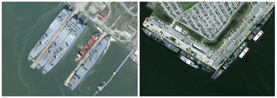
Figure 1.
Objects in aerial images display diverse morphological and distributional features, including arbitrary orientation, multi-scale, and high aspect ratio.
In order to tackle comparable difficulties, follow-up studies have concentrated on correcting horizontal anchors to oriented anchors and carrying out region alignment. As an illustration, R3Det [] utilizes a method similar to RROI Pooling to re-encode the location information of the adjusted horizontal anchor into matching feature points. This process involves pixel-level feature interpolation, resulting in feature reconstruction and alignment. However, the RoI transformer [] determines positive and negative samples by computing the Intersection over Union (IoU) between a horizontal anchor and the smallest rectangle that envelopes the ground truth (GT) box. This process helps train high-quality horizontal CRBs. Next, they acquire oriented CRBs through regression and use RRoI Align to accurately correct the regions’ features for alignment. Although R3Det and RoI Transformer do not necessitate a substantial quantity of predefined anchors, they nonetheless demand the heuristic establishment of horizontal anchors and the execution of intricate RRoI computations. All the methods mentioned above utilize traditional CNNs to extract TEFs. They create an approximation of rotation invariance by using RROI Pooling or RRoI Align to simulate changes in rotation [].
Although the features and objects have been successfully aligned, the design concept of the backbone bears resemblance to RRPN, R3Det, and RoI Transformer. These methods rely on a backbone made of stacked fixed and small receptive field kernels. However, they do not effectively utilize the contextual information surrounding the target. As a result, the constraints that arise include a restricted ability to adjust to different scales and a vulnerability to background noise interference. For oriented object detection to work well on multi-scale objects, more complex, deeper networks and training data are usually required to obtain more robust scale representations. Nonetheless, this leads to more intricate network structures and increased computational complexity, which presents obstacles to deploy.
The analysis shows that to accurately and rapidly detect remote sensing objects of various scales, it is necessary to utilize the object’s distinctive features and contextual background information while ensuring consistency in the task. Currently, we can categorize the problems in remote sensing object detection into three types, spatial misalignment, feature misalignment, and task misalignment, as shown in Figure 2. They are described as follows.
- Spatial Misalignment Issue. Existing networks use a convolution kernel structure with a fixed and small kernel size, which can be misaligned in terms of spatial alignment, thus making it difficult to align the spatial coverage of objects and accurately perceive changes in scale and orientation. In order to expand the receptive field, current remote sensing detectors need to stack more small convolution kernels, which leads to a more complex network and a heavier computational load. In addition, a fixed and narrow receptive field reduces the detection accuracy because it cannot recognize objects precisely. The reason for this limitation is that accurate target detection usually relies on a large and changing amount of contextual information about the target environment, which can provide essential insights into the target’s shape, location, and other characteristics.
- Feature Misalignment Issue. The normal convolution operation moves in a horizontal direction, and the TEFs are extracted. However, the RIFs required to recognize rotating targets effectively make it difficult to identify objects with specific orientations, causing feature misalignment and lower detection accuracy. Furthermore, when the convolution’s sliding direction does not align with the target orientation, it introduces background noise of varying intensities, disrupting the extraction of the TEF. This makes it challenging to obtain a satisfactory target representation, making the detection accuracy even worse.
- Task Misalignment Issue. The classification task requires RIFs, while the regression task requires orientation-sensitive features (OSFs). However, the classification/regression branch in the detection head directly uses the fusion features of the anchor network and FPN for the object classification and localization tasks, which may lead to inconsistencies in the final classification confidence score and regression localization accuracy. More precisely, the anchor point has to face the awkward situation of low localization accuracy while having a high classification score. On the contrary, the nonmaximal suppression (NMS) stage may abandon objects with higher localization accuracy due to lower classification scores, leading to missed detections. Therefore, the inter-task misalignment problem can seriously affect the detection accuracy.
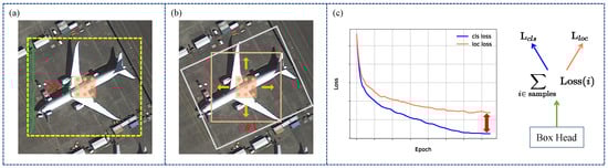
Figure 2.
(a) Spatial misalignment between the fixed receptive field with a kernel size of 3 × 3 and the range (yellow rectangle) of contextual information required to detect the object accurately. (b) Feature misalignment exists between the oriented anchor (grey rectangle) and the convolution features (red-beige rectangle). (c) Shared backbone features result in task misalignment between classification and regression.
In order to tackle the above problems, this study has proposed a Staged Adaptive Alignment Detector (SAADet), which first utilizes the proposed SSANet backbone network to dynamically evaluate the scale-sensitive contextual features extracted by different receptive field size convolution kernels based on the input with the aid of a spatial selection mechanism; second, after correcting the horizontal anchor to the oriented anchor, the spatial features are extracted by guiding the alignment convolution (AC) [] to align with the object orientation; and finally, the alignment features decouple into RIFs and OSFs through the Active Rotation Filter (ARN) [].
Our method performs robustly on two remote sensing datasets—HRSC2016 and UCAS-AOD. They are publicly available. Specifically, this study has resulted in the following contributions:
- We propose a lightweight backbone network to achieve adaptive spatial selection and thereby acquire extensive and dynamic contextual information to enable spatial alignment.
- RIFs are obtained by correcting the horizontal anchor regression to an oriented anchor to guide the AC to complete the feature alignment by moving from a coarse to a delicate detection pattern.
- We propose an efficient feature decoupling method to perform task alignment and mitigate the inconsistency in classification and regression.
2. Related Work
2.1. Oriented Object Detection
In remote sensing, real-world scenarios present various challenges for object identification, including the presence of rotated objects with multiple orientations. Conventional detection networks that rely on CNNs are inefficient in detecting objects with specific orientations because they do not possess rotation invariance (RI). Research efforts have primarily focused on developing detection algorithms that can accurately capture the orientation features of objects.
In order to recognize rotating multi-oriented objects, researchers have made substantial efforts to improve the feature representation of conventional networks. For example, Cheng et al. [] inserted a rotation-invariant layer into AlexNet []. Ensuring that the feature representations of the samples are similar before and after the rotation during the training process made it easier for the detector to find objects positioned differently. They achieved this by applying regularization constraints in the objective function. Shi et al. [] devised a geometric transformation module that produces images from different perspectives using random rotations and flips. This allows the detector to acquire knowledge about oriented features effectively. In their study, Huang et al. [] utilized a Deformable Convolution module to obtain RIFs, thus resolving the problem of recognizing rotated objects.
However, the studies above rely on horizontal anchors established by axis alignment. While these anchors improve the convolution network’s ability to represent oriented features, they cannot effectively capture the object’s orientation information. Horizontal anchors cannot precisely indicate an object’s orientation, namely, the rotation angle. Furthermore, objects tightly packed together pose challenges for horizontal anchors. The significant overlap between anchors can easily cause anchor suppression during postprocessing, leading to missed detections. As a result, researchers have pursued new avenues of investigation in anchor detection. We can broadly classify these investigations into three types: redundant oriented anchor, angle regression, and representation of oriented anchor.
Presetting Redundant Oriented Anchor. This method entails predefining numerous oriented anchors at every place in the feature map to align with objects of specific orientations without modifying the current network structure. One can achieve this by altering the angle information of the anchor hyperparameters. Ma et al. [] first proposed a Rotating Region Network for creating anchors with orientation. This led to the widespread adoption of the idea of using preset-oriented anchors. Liu et al. [] utilized a 12-angle oriented anchor and suggested substituting the angular loss regression with the diagonal length of the bounding box, which led to positive outcomes. In order to mitigate the problem arising from little variations in the angle of the object, Bao et al. [] developed the ArIoU metric to improve the reliability of its evaluation, particularly for tiny angles. Meanwhile, Xiao et al. [] presented a method for anchor selection, which adaptively allocates anchors and constructs anchors with six angles at each point to accurately locate targets with specific orientations.
Design Angle Regression. This method uses a regression function to predict the object’s orientation, where the angle information is not combined with the position information of the four boundary corner points of the anchor but is regressed separately. For instance, Yang et al. [] developed a multi-task rotating region CNN that directly predicts the ship’s sailing orientation through successive modules such as oriented anchor regression, bow orientation prediction, and rotated nonmaximum suppression. Conversely, Hua et al. [] utilized a point-wise convolution to predict the orientation and designed a new angular loss function for constraints. Additionally, some researchers [,,] also implemented horizontal and oriented prediction heads at the late stage of the detection, generating horizontal anchors and oriented anchors simultaneously. To address the issue of boundary mutations in oriented boxes, Chen et al. [] proposed the Oriented Bounding Box Multi-Definition and Selection Strategy, resulting in smoother regression of the oriented anchor and the more accurate detection of oriented objects.
Enhancing the Representation of Oriented Anchor. In real-world scenarios, RRoI Warping [,] (such as RRoI Pooling and RRoI Align) is widely employed to extract RIFs from the two-dimensional plane. This method correctly warps regional features based on the anchor’s RRoI. However, using regular CNNs for RRoI Warping cannot get a real sense of the RIFs and accurately model orientation changes, a network with a higher capacity and a larger number of training samples is required to achieve an RI approximation. ReDet integrates RE operations [] into the backbone feature extractor to produce REFs. It then utilizes RiRoI Align to selectively extract RIFs from the REFs. Pu et al. [] introduced the Adaptive Rotated Convolution (ARC) kernel, which is designed to extract object features with varying orientations in images. They also implemented an efficient conditional computation method to adjust to changes in the object orientation inside the image.
2.2. Deformable Convolution
In order to accurately predict targets in aerial images, their rotated multi-orientation, multi-scale, and effective representation of the high aspect ratio need to be considered. General research efforts usually model the deformation of these targets from transform-invariant feature operators and CNNs. These methods have inherent drawbacks because they usually give geometric deformations that are fixed and known a priori, which makes them unable to cope with the new task of unknown geometric deformations. Second, manually designed invariant features and fixed-size convolution kernel templates require the addition of extra aids in order to be able to cope with a wide variety of complex deformations.
In order to reinforce the modeling capability of objects with multi-scale and high aspect ratios, Dai et al. [] introduced Deformable Convolution Networks (DCNs). DCN incorporates learnable offsets, allowing the convolution kernel to adjust its shape and position better to accommodate the geometric variations in the input data. DCN improves the detector’s ability to perceive changes in the shape of targets, thereby increasing object recognition and localization accuracy. Furthermore, Zhu et al. [] proposed an upgraded version of Deformable Convolution Networks (DCNv2) that incorporates extra trainable parameters to alter the shape of the convolution filter. This modification enhances the network’s capacity for modeling and training, resulting in improved attention to essential regions in images. The DCNv2 model has superior accuracy and resilience in handling distorted objects.
Furthermore, Wu et al. [] proposed Dynamic Filter Networks (DFNs), which enable the convolution kernel to apply different filter weights at various locations by introducing dynamic filters. This method enables the convolution process to adjust to variations in the local structure of the input data in real time, enhancing feature detection. There is also a method called Dynamic Convolution (DynamicConv), proposed by Zhao et al. [], which introduces a dynamic deformation field to enable the convolution kernel to adapt to the geometric changes of the input image dynamically. DynamicConv can extract more distinctive features and utilize varying filter weights across different input image regions, leading to a scaled-up performance in classification and detection tasks.
Nevertheless, Deformable Convolution has certain drawbacks. Incorporating learnable offsets amplifies the intricacy and computing burden of the model, potentially leading to extended durations for both training and prediction processes. Furthermore, tuning the parameters of Deformable Convolution demands a higher level of expertise and proficiency. In addition, Deformable Convolution may lack accuracy when dealing with tiny objects or intricate features.
3. Methodology
Figure 3 showcases the introduction of a Staged Adaptive Alignment Detector (SAADet) explicitly designed for object detection in aerial images. The three main components of SAADet are the backbone, neck, and head. The backbone component utilizes our proposed spatial alignment adaptive network (SSANet) for feature extraction and acquires feature maps of diverse semantic levels by sequential downsampling. Shallow features encompass coarse-grained spatial information, while deep features contain fine-grained semantic information related to the object categories. The neck utilizes the FPN structure. It upsamples the resolution of feature maps coming in from different backbone layers, then combines them with feature maps from the same layer to restore spatial resolution and gather more contextual information. This allows for capturing the features of objects at multi-scale. The head consists of five detection heads accountable for the classification and anchor regression of different-scale objects using the feature maps yielded from the neck. Each detection head consists of two modules, AGCM and RDM. AGCM is responsible for correcting the horizontal anchor to an oriented anchor, which guides the AC to align the axis-aligned features to an arbitrarily oriented object after correction. RDM employs ARFs to decouple the aligned features into RIFs and OSFs, thereby mitigating the inconsistency between object classification and positional regression.
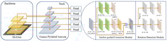
Figure 3.
Structure of the proposed SAADet. The SAADet system consists of an SSANet backbone, a Feature Pyramid Network (FPN) [], an Anchor-guided Correction Module (AGCM) and a Rotation Detection Module (RDM). Detection heads, consisting of AGCM and RDM, operate at every scale level of the feature pyramid. AGCM uses the Anchor Refinement Network (ARN) to correct the preset horizontal anchor to generate a high-quality rotated anchor. We then feed the rotated anchors and features into the AC Layer (ACL) to obtain the aligned features. The RDM uses Active Rotating Filters (ARFs) [] to decouple the aligned features into rotation-sensitive features (RSFs) and RIFs. Then, the cls. branch and reg. branch yield the final detections.
3.1. SSANet Backbone Architecture
A bird’s-eye view of targets on the ground from a high altitude reveals significant scale differences in their appearance. Suppose valid contextual information about the surrounding background and environment closely linked to these targets can be obtained. In that case, a better understanding of their shape, orientation and scale can be achieved, enabling more effective and accurate predictions. Conventional CNNs, constructed by stacking small and fixed convolution kernels, struggle to comprehend the entire scene and accurately identify objects based on limited or local features. However, the computing burden is significantly increased if we stack multiple small convolution kernels to achieve a larger receptive field. In order to tackle this issue, we introduce the SSANet backbone network as seen in Figure 4a to extract comprehensive and adaptable contextual information while ensuring a streamlined network architecture.
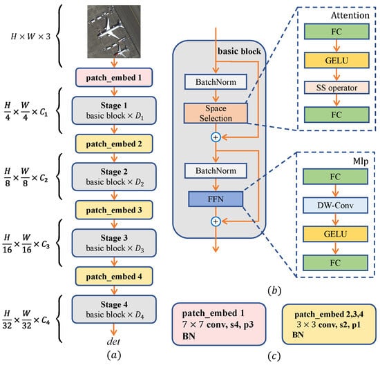
Figure 4.
(a) The overall architecture of SSANet. (b) Detailed illustration of the basic block. SS operator as its core operator. Each basic block comprises batch normalization, attention-based Space Selection, and a feed-forward network (FFN). (c) The patch-embedding layers follow conventional CNN designs. As seen in patch-embed 1, ‘s4’ and ‘p3’ represent stride 4 and padding 3, respectively.
The SSANet architecture is primarily based on a stacking basic block structure. As shown in Figure 4b, each basic block has two residual sub-blocks: the Space Selection sub-block is in the front, followed by the FFN sub-block. The SS operator, seen in Figure 5, is the core component of SSANet and implements the spatial attention mechanism through Space Selection. Based on the inputs in a learnable manner, this operator dynamically evaluates the importance of the feature maps of multiple different depth kernels. The corresponding attention scores are obtained to perform a weighted summation of these feature maps. The operator can adaptively select kernels with different receptive fields according to different targets. The FFN sub-block’s design utilizes large kernels with different receptive fields adaptively. The FFN sub-block introduces more complex nonlinear relationships that map features from the input dimension to higher-dimensional latent spaces, augmenting the expressive power of the model and aiding the model in better learning higher-order representations of the input features, as well as understanding and capturing the subtleties and correlations in the input features.
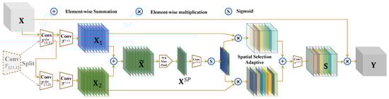
Figure 5.
Detailed conceptual illustration of the SS operator, visualizing the operation of the spatial selection mechanism. Specifically, the SS operator enables the network to dynamically select appropriate large receptive field features based on different objects. The underlying principle of this design is that choosing receptive fields with different dimensions makes it possible to collect contextual information at various scales. This, in turn, aids in recognizing objects of varying sizes and shapes. The SS operator can efficiently adjust to complicated situations and objects by selectively choosing receptive fields. This strategy of splitting a singe oversized kernel convolutions also tackles the issue of a substantial rise in parameter quantity.
Further clarification is needed; the last layer of FC in the Space Selection sub-block is not a traditional fully connected one but a point-wise convolution. Point-wise convolution is a typical convolution operator used in CNNs. It is often used to reduce or expand the number of channels of a feature map or for feature fusion; it can replace the role of a fully connected layer. This is because it has few parameters and can reduce the number of parameters by controlling the number of output channels, reducing the model’s complexity and computational cost. In contrast, the fully connected layer requires many parameters, which can easily lead to overfitting and computational burden.
The patch_embed downsampling layer is used to acquire hierarchical feature maps as depicted in Figure 4c. The patch_embed layer is placed before the stage layer to downsample the image’s input resolution by a factor of four. Similarly, the patch_embed layer applies downsampling to input feature maps by reducing their size by half using 2, 3, and 4 layers.
The stacking of basic blocks in SSANet is impacted by ConvNeXt [], PVT-v2 [], VAN [], ConvFormer [], metaFormer [], and LSKNet [] models. The organization method is specified in Table 1, where the hyperparameter denotes the number of feature channels in the ith stage layer, and indicates the number of basic blocks in the ith stage. The SSANet model we propose consists of only two versions, requiring eight hyperparameters to describe its structure.

Table 1.
Versions of SSANet in this study. The variable denotes the number of feature channels, and denotes the number of basic blocks in the ith stage.
3.2. Mechanisms for Adaptive Spatial Selection
A wide receptive field is essential for tasks involving target recognition. Nevertheless, merely extending the size of the receptive field results in an escalation of the parameter quantity and computing complexity. This method may not adequately cater to the dynamic and broad range of contexts required for precise object recognition.
Recent studies have shown that well-designed convolutional networks with large receptive fields can achieve performance similar to that of Transformer []-based models. ConvNeXt [] embeds deep convolutions in its backbone, significantly improving downstream tasks’ performance. RepLKNet [] also achieved surprising performance by reparameterizing using a convolution kernel. SLaK [] further expanded the kernel to by decomposing the convolution kernel and sparse grouping methods. The decomposition of the large kernel of VAN [] performs an efficient decomposition to form the convolutional attention.
In order to address the difficulties raised at the beginning of this sub-section, according to the above technical line, we suggest directly splitting a single oversized kernel into a sequential succession of deep convolution kernels. These kernels have progressively increasing size and dilatation rates, allowing for contextual information extraction at different scales. For example, the oversized kernel with a kernel size of 23 and dilation rate of 1 is split into two large kernels. The first large kernel of the splitting has a kernel size of 5 and a dilation rate of 1. The second large kernel has a kernel size of 7 and a dilation rate of 3. The theoretical receptive field is unchanged before and after the splitting. After splitting the two large kernels, which are connected serially, their respective feature maps are subjected to attention weight calculation, and the features of the more critical kernels are dynamically selected for weighted reinforcement according to different inputs X to realize the spatial attention mechanism and achieve the purpose of spatial feature adaptive selection. Equation (1) expresses the ith deep kernel receptive field calculation in the kernel series after splitting the single oversized kernel:
To avoid creating gaps between feature maps, we set a maximum limit on the dilation rate in convolution. For example, we can split a single oversized kernel into two or three smaller kernels as shown in Table 2; the two oversized kernels have a theoretical receptive field size of 23 or 29, respectively. This splitting strategy has two significant advantages. First, it directly evaluates the importance of different kernels based on input with distinct receptive fields, allowing for adaptability in spatial selection and the ability to collect features at various scales and splitting a single oversized kernel into consecutive large kernels with greater efficiency than using a single oversized kernel. As shown in Table 2, our splitting strategy effectively decreases the parameter count for an equivalent theoretical receptive field compared to a single oversized kernel.
Table 2.
The splitting of a single oversized kernel into deep kernel sequences (assuming 64 channels), assessing the number of parameters and floating-point operations for two common scenarios. Here, the variable ‘k’ represents the kernel size, whereas ‘d’ represents the dilation rate.
Given a split sequence consisting of N depth kernels , each kernel is then followed by a convolution kernel , that is
The function indicates that the kernel size of the deep convolution is k and the dilation rate is d.
This design performs channel fusion for each spatial feature vector. With the convolution layer, we could transform and adjust the channel dimensions to better suit different object tasks and scenarios.
We make a spatial selection adaptive mechanism to help the detector capture the most exciting area of spatial context, stop from looking at the global context, and only look at the context around each object’s position, which lowers the effect of areas that are not relevant. This mechanism selects extensive kernel features with varying scales. To be more precise, we first perform an element-wise summation of features captured from various kernels with different receptive field ranges:
where ⨁ denotes element-wise summation.
To effectively process the spatially pooled features from in the channel dimension, we utilize average and maximum pooling, represented as and . Afterwards, we link these combined features in the channel dimension. In order to enhance the interaction among various pooling features, we utilize a convolution layer to convert them into N distinct spatial attention maps. This allows for the merging and interaction of spatial data at different levels, resulting in a more varied and impactful spatial attention map :
To accomplish spatial selection adaptivity, we employ a sigmoid activation function to calculate the mask for . Afterwards, we evaluate and weigh the features of through the mask and carry out an element-wise summation of the N-weighted feature maps over the channel dimension. Next, channel fusion is performed using the 1 × 1 convolution kernel to provide a score , which represents spatial attention:
The symbol denotes the sigmoid function, whereas ⨂ denotes element-wise multiplication.
The output of the SS operator is created by performing element-wise multiplication between the input features and , which is similar to the method described in [,,]:
Figure 5 presents a comprehensive conceptual depiction of an SS operator, showcasing a clear explanation of how the spatial selection mechanism effectively captures the appropriate broad receptive field for various objects in an adaptive manner.
3.3. Anchor-Guided Correction Module (AGCM)
Anchor Refinement Net. Conventional object detectors that rely on anchors have difficulty accurately detecting objects with different scales and orientations. In order to tackle this issue, we propose a lightweight Anchor Refinement Network (ARN) that consists of two simultaneous branches: one for anchor classification and another for anchor regression. The first branch sorts an anchor into two categories: foreground and background, whereas the second branch refines horizontal anchors to high-quality oriented anchors as indicated by the blue arrows in Figure 3. We only require the regressed oriented anchor to guide AC in adjusting the sampling position during the training stage. Consequently, the inference phase eliminates the classification branch. Utilizing the one-to-one design of the anchorless detector, we introduce a singular square anchor for every place in the feature map. Furthermore, we do not exclude class predictions with low confidence, as the final forecast reveals certain negative class predictions to be positive.
Aligned Convolution. A common 2D convolution computational procedure is illustrated here. denote the input and output feature map, respectively, and the position of each point on takes the value of the domain . First, we use a standard grid for sampling, where . Next, the sampled values are combined using a weighted summation with the matrix . The grid which means that a kernel size is 3 and a dilation rate is 1. For every point in the domain on , we have
Compared with common convolution, AC introduces an offset scope, represented as , at each point :
The offset scope () is determined by comparing the sampling position of the anchor with the usual sampling position () for a given location (). Denote the coordinates of the appropriate anchor at point () as (). The anchor-based sampling position () is defined for each () as follows:
where k denotes the size of the kernel, S denotes the stride of the feature map, and is a matrix defined as represents a rotation. The offset scope at the position is defined as
This way, we can convert a given position according to an axis-alignment convolution feature’s corresponding oriented anchor p into an arbitrarily oriented feature.
We propose AC to extract features of the mesh distribution by adding an extra offset scope guided by an oriented anchor. Unlike Deformable Convolution, the offset scopes in AC do not need to be learned but can be inferred directly from the oriented anchor.
Aligned Convolution Layer. After introducing the AC, we developed an Aligned Convolution Layer (ACL) as shown in Figure 6. First, we decoded the anchor prediction grid with dimensions of into absolute anchor coordinates denoted by (). We then determined the offset scope by applying Equation (10). This offset scope was then combined with the input features in the AC to extract the alignment features. We must highlight that we employed a uniform sampling method for every anchor (with 5 dimensions) to collect points (with 3 rows and 3 columns). This allowed us to acquire an offset scope with 18 dimensions (consisting of 9 coordinates for both x and y offsets). Blue arrows represent these coordinates in the diagram. Additionally, it is essential to highlight that ACL functions as a lightweight convolutional layer with minimal computational delay in determining the offset scope.
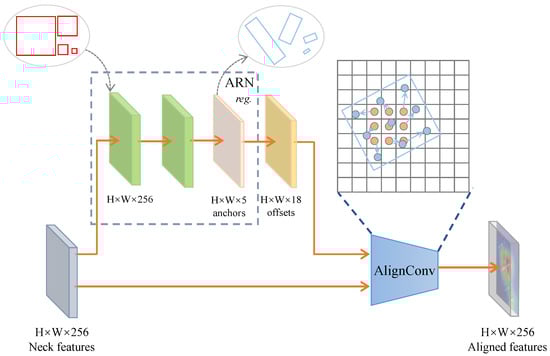
Figure 6.
Elaborate conceptual depiction of the AGCM module. The ARN corrects the initial horizontal anchor to an oriented anchor, which guides the AC to complete the feature alignment of the Neck features to the object.
3.4. Rotation Detection Module (RDM)
We used RetinaNet as our baseline model, integrating its architectural design.
Feature Decoupling. To fix the problem of the irrelevance between predictive classification and localization regression, we added a feature decoupling module (RDM), as seen in Figure 3, to make object detection more accurate. At first, we employed ARF to encode the angle information. The ARF is a kernel with dimensions. It is rotated times during convolution to produce Y with N angle channels. The default value for N is 8. As far as a X and the ARF are concerned, convolved with the ARF , the nth rotation result of Y can be represented as follows:
The notation represents the clockwise rotation of by an angle of . Similarly, and refer to the ith individual channel orientations of and , respectively. We successfully acquired RSFs containing clear and specific angular information encoding by implementing ARF on the convolution layer.
Regression tasks need OSFs, whereas object classification tasks demand RIFs. The objective of our study as stated in the literature [] is to extract RIFs by pooling OSFs. The method is direct: choose the orientation channel that shows the most significant reaction as the output feature,
We can improve the object classification accuracy and reliability by aligning object features with different orientations. RIFs necessitate fewer and more efficient parameters in comparison to rotation-sensitive features. After combining the dimensions of height (H), width (W), and 256, a feature map with 8 orientation channels will have the dimensions of . Afterwards, we pass on to the rotation-sensitive and rotation-independent features in two separate sub-networks to forecast the positions and the categories.
Regression Targets. Each oriented anchor is represented as a quintuple (), where x and y represent the center coordinates, w and h designate the width and height dimensions, and () denotes the angle concerning the horizontal. The regression process aims to forecast the offset between each positive anchor and the adjacent GT. In order to provide regression invariance of scale and position, the offset vector () is commonly parameterized as follows:
The symbols and represent the anchor and its GT, respectively. The integer k ensures that the rotation of the anchor and its GT, given by , falls within the range of .
In AGCM, we set to represent the level anchor. Subsequently, the regression object can be represented by Equation (15). In RDM, we initially decode the final output of the regression branch and then recalculate the regression object by Equation (15).
Strategy for matching. We employ the IoU as the metric to evaluate the effectiveness of our matching method. An anchor is considered positive if its IoU value exceeds the foreground threshold. On the other hand, we label an anchor as negative if its IoU value falls below the background threshold. Contrary to the IoU calculation for horizontal anchors, we compute the IoU for two oriented anchors. In AGCM and RDM, establishing the foreground and background thresholds to 0.5 and 0.4 is customary, respectively.
The multi-task loss function. The SAADet loss is a comprehensive loss function that combines the loss of AGCM and RDM, consisting of two components. For every horizontal anchor/oriented anchor, we assign a category label to each component and determine its position by regression. We explicitly define the loss function as follows:
Here, represents the loss balance hyperparameter, denotes the indicator function, and refer to the number of positive anchors in AGCM and RDM, respectively, and i represents the index of the samples in the mini-batch. and indicate the index of the ith sample prediction category and correction location in AGCM, whereas and represent the predicted object category and ith sample position in the RDM. The variables and denote the proper category and position of the object, respectively.
4. Experimentation
4.1. Datasets
We conducted tests using two publicly accessible remote sensing datasets, HRSC2016 and UCAS-AOD, both annotated with oriented GT boxes.
HRSC2016 [] is an extensive dataset specially designed for aerial ship detection. It is made up of 1061 photos with sizes that vary from to . We divided these photos into 436 for the training set, 181 for the validation and 444 for the test set. Dense distribution, diverse scales, complex image backgrounds, and high similarity between the ship and the near-shore texture characterize the area along the shore. In order to maintain consistency in our experimentations, we adjusted the size of the images to for both training and testing to focus on a single scale.
The UCAS-AOD [] dataset is an aerial image dataset designed for detecting two types of objects: cars and airplanes. All images are captured from various global regions using Google Earth. This dataset comprises approximately 2420 images with a total of 14,596 instances, and the image sizes range from to pixels. These images depict diverse types of cars and airplanes in various environmental conditions, including different lighting, weather, and seasonal variations. The dataset exhibits a diverse distribution of targets, encompassing various models, colors, and sizes of cars and airplanes, as well as their distributions in different environments such as airport runways, parking lots, and urban streets.
4.2. Evaluation Metrics
The standard evaluation metrics for object detection are Recall, Precision, Average Precision, Precision–Recall Curve, mean Average Precision, and frames per second. The above metrics are abbreviated below: R, P, AP, PRC, mAP, and FPS. The first five metrics evaluate detection accuracy, whilst the final metric evaluates the detection speed.
The IoU measures the proportion of overlap between the predicted box and the GT box regarding their total area. It serves as an indicator of the accuracy of object identification. We explicitly define the IoU as follows:
The classifications are determined based on the following outcomes: True Positive, False Negative, False Positive, and True Negative. The above outcomes are abbreviated below: TP, FN, TP, and FP. Recall and Precision are defined as the following:
The addition of True Positives and False Negatives represents the total number of GT boxes. In contrast, the sum of True and False Positives reveals the number of objects that have been predicted as positive. Therefore, the number of accurately predicted objects out of the total detected objects determines P, and the number of correctly predicted objects out of the total actual objects determines R. AP, or Average Precision, is a metric that considers both Precision and Recall. It is defined as follows:
AP represents the Recall’s average precision, which ranges from 0 to 1. We obtain the PRC, a graphical representation, by determining the maximum P value for each R. The area of the region under the graph is the AP. We calculate mAP, or mean Average Precision, by taking the average precision across all categories. We represent it using the following formula:
The mAP is a metric that measures the accuracy of object detection. The value of N denotes the number of different target categories being considered. Therefore, a higher mAP score suggests a more accurate and exact detector.
Aside from examining accuracy, the speed of detection is also a crucial component in thoroughly evaluating the detection performance. Commonly, we quantify the speed of detection in frames per second (FPS), indicating the number of samples we can recognize in a single second. The duration required to process the photos can also quantify the speed.
4.3. Implementation Details
Multi-scale object detection is achieved by utilizing the P3, P4, P5, P6, and P7 layers of the feature pyramid. We assign a single anchor to each point on the feature map to predict neighboring objects. This study utilizes random flips as a means of augmenting the data. To ensure high-quality detection, we set the positive example match threshold in AGCM at 0.5 and RDM at 0.5.
This study adapts the mAP as the metric for evaluation. We use the mAP metric from the PASCAL VOC 2007 Challenge for the HRSC2016 and UCAS-AOD to compare with other methods. We carry out a series of ablation experiments on the HRSC2016, known for its vast variations in aspect ratio and scale in remote-sensing images of ships. These variations provide a considerable barrier to object detection in aerial images.
We train and test the model at a single scale using only one RTX 2080Ti graphics card. The network is trained to adopt the Stochastic Gradient Descent (SGD). We set the batch size and initial learning rate of SGD to 8, 2.5 × 10⁻³, respectively. The momentum value is set to 0.9, while the weight decay value is set to 0.0001. We train 48 and 24 epochs on HRSC2016 and UCAS-AOD, respectively. The input samples for the HRSC2016 and UCAS-AOD have a resolution of 800 × 800. In this study, all experiments are performed using the framework of oriented object detection MMRotate.
4.4. Ablation Studies
The selected baseline consists of the ResNet backbone and the RetinaNet detector. The backbones of our proposed methods all adapt SSANet-S in ablation studies.
Assessing the validity of different versions of SSANet. The performance of the network is affected by its depth and width; the depth is reflected in the stacking of convolution kernels, i.e., the stacking of basic blocks, and the width is expressed in the number of channels in the convolution kernel. The depth of SSANet-T is slightly larger than that of SSANet-S. However, as shown in Table 3, the width is halved in each stage, which results in insufficient fusion of the features in the channel dimension, and so it lags in the final mAP metrics by 1.45%. So in this study, we use SSANet-S.
Table 3.
Comparison of detection mPA for two versions of SSANet backbone networks, SSANet-S and SSANet-T.
Evaluation of different splitting styles for a single oversized kernel. The number of kernels after splitting is an important factor for the SS operator. We implement the splitting strategy based on Equation (1). We thoroughly examine the impact on performance when breaking down a oversized kernel into multiple kernels of varying depths. We conduct this study assuming a fixed receptive field size of 29. As shown in Table 4, The results show that splitting an single oversized kernel into two smaller depth kernels can achieve equilibrium in speed and accuracy, resulting in the best FPS and mAP performance.
Table 4.
This study examines the impact of varying numbers of splits on inference FPS and mAP, assuming a theoretical receptive field of 29. The trials illustrate that the process of breaking a single oversized kernel into two smaller, more concentrated kernels effectively preserves both performance and precision.
A single oversized kernel suffers from too many parameters, high computational complexity, and slow inference, and its fixed receptive field may also intensify spatial misalignment with the object, affecting the detection accuracy. In contrast, splitting the oversized kernel into more kernels, although it will increase the number of parameters by a small amount, which will have some impact on the performance, the bigger problem is that more kernels will lead to a relatively more minor corresponding receptive field, which will not allow the object to efficiently and dynamically select the required contextual information, which in turn will have an impact on the detection accuracy.
Validity of receptive field size and selection type. The findings in Table 5 indicate that a receptive field size of 23 produces the most optimal outcomes. The size of the receptive field is critical in object appearance matching and identification. A limited receptive field can result in the inadequate extraction of the object’s features and important contextual information, impeding precise object recognition. On the contrary, if the receptive field is too big, it might cause more noise because of the increased distance and extra space. This can lead to the noise overshadowing smaller and medium-sized objects. Furthermore, an excessively expansive receptive field can cause the model to incorrectly see background noise as a component of the object, reducing accuracy and resulting in missed detections. As a result, there is a compromise in determining the receptive field size, ensuring sufficient background information is retained while effectively capturing object features.
Table 5.
The effectiveness of ablation study is assessed by examining the impact of different receptive field sizes and selection types while using a single oversized kernel that is separated into two depth kernels in a sequence. CS (Channel Selection) is analogous to SKNet []. On the other hand, SS (Spatial Selection) is a method that we have developed and put forward. We achieved the optimal performance of SSANet by using spatial selection to obtain a large receptive field adapted to the target.
Furthermore, the empirical results in Table 5 demonstrate that our suggested spatial selection method surpasses channel attention methods (such as SKNet) in aerial object detection tasks. The spatial selection method’s superiority stems from its ability to accurately represent the scale and shape of various targets in aerial images, which frequently exhibits significant differences in object scale and shape. Conversely, conventional channel attention mechanisms exclusively concentrate on the channel dimension’s feature response, disregarding the objects’ distribution in the image space. Our spatial selection method can more precisely capture position and shape information by accurately simulating distinct objects’ spatial scales and aspect ratios.
Comparing the Efficacy of Maximum Pooling and Average Pooling. When looking at how well max pooling and mean pooling work in CNNs, it is clear that both reduce the number of dimensions in the feature map, make the model run faster, and use less computing power. Max pooling is a highly successful method for recognizing key aspects of an image, such as edges and textures. This process significantly improves the model’s capability to detect and recognize crucial features. Conversely, average pooling effectively reduces noise and fine details in the image while retaining more background information, making it well suited for jobs that involve recognizing backgrounds and understanding scenes.
As is evident from Table 6, combining maximum pooling and average pooling improves detection accuracy by 1.06% and 1.97%, respectively, compared to using only one pooling method. By utilizing this integrated method, the model can extract contextual information at several scales more efficiently, resulting in enhanced accuracy in object detection.
Table 6.
A study examining the influence of maximum and average pooling on spatial selection in the SSANet backbone we developed. The results suggest that using both maximum and average pooling simultaneously yields the best outcomes.
We conducted a study to examine the impact of several combinations, including SSANet, AGCM, and RDM of SAADet, on performance. Our findings revealed that the SSANet backbone is effective in the spatial selection mechanism.
Assessing the validity of different components of SAADet. To determine the validity of the proposed components, we performed component configuration experiments on the HRSC2016. Table 7 displays the mAP results of the experiment. At first, because of the preset one anchor box and the challenge of capturing the critical features needed for object detection, the baseline model attained a mAP level of 74.16%. Adding SSANet made detection work 4.66% better, which suggests that the SSANet backbone network was able to obtain more accurate feature representations. Despite having only one preset anchor, AGCM efficiently utilized the critical features to correct the horizontal anchor accurately during the learning process, resulting in a 5.21% enhancement in detection performance. After that, SAADet obtained a 6.69% improvement in detection performance by using the aligned features decoupling method called ADM. This is a significant increase of 16.56% improvement compared with the baseline model. This very visual demonstrates the effectiveness of our suggested SAADet.
Table 7.
The outcomes of the ablation study on the detection performance for various combinations of SAADet components. SAADet delivers optimal performance by effectively combining SSANet, AGCM, and RDM to align at the spatial, feature, and task levels.
Impact of variable numbers of ARN stacking on performance. This section examines how different numbers of ARN stacking, i.e., the number of correction steps, affect performance. The model sans ARNs used a matching threshold of 0.4 for positive cases during the detection phase. The one-stage ARN component set the thresholds for the correction and detection stages at 0.5. We established the two-stage ARN component threshold at 0.4, 0.5, and 0.7. Table 8 illustrates a 4.44% enhancement in performance achieved by utilizing the one-stage ARN. This improvement can be credited to replacing horizontal anchors with orientated anchors, which results in the model being provided with superior samples more accurately aligned with the object’s critical features. Nevertheless, utilizing a two-stage ARN led to a decrease in performance of 1.26% compared to a one-stage ARN. Raising the threshold during the detection phase can substantially decrease the number of positive anchors that surpass the existing matching threshold. This can lead to a scarcity of positive anchors and a pronounced imbalance between positive and negative anchors. Therefore, the detection header employs a single-stage ARN.
Table 8.
The ablation study evaluates the effectiveness of different correction stages when employing ARN for anchor correction. The study shows that the best performance is attained with one-stage refinement.
4.5. Comparative Experiments
The backbones of our proposed methods all use SSANet-S in comparative experiments.
HRSC2016 Results. Our method achieves the highest ranking with an outstanding mAP of 90.72% on the HRSC2016 as shown in Table 9. Significantly, our method utilizes a single horizontal anchor at every position on the feature map, leading to quicker inference and surpassing frameworks that depend on many superfluous predetermined anchors. These data indicate that using several anchors is unnecessary for efficient oriented object recognition. By configuring the input image size to pixels, our model significantly improves 17 frames per second on the RTX 2080 Ti GPU, showcasing outstanding real-time performance. Figure 7 is provided below. Our method effectively demonstrates the detection outcomes on the HRSC2016, providing clear visual insights.
Table 9.
Comparison of mAP values achieved using different methods on the HRSC2016. The highlighted numbers in the table represent the highest mAP scores achieved compared to all other methods.
Figure 7.
Visual demonstration of the final detection results of different categories on HRSC2016 adapting our method. Due to the high resolution of the image, please zoom in to view the test results.
Results on UCAS-AOD. The results of our proposed method are analyzed in Table 10, where it achieves a mAP of 90.47%. This ranks it at the top and shows a clear advantage over other detectors. Figure 8 visualizes the detection results on the UCAS-AOD dataset. The detection results highlight the importance of aligning spatial, feature, and task levels to achieve precise rotated object detection. From Figure 8, it can be observed that both the dense distribution of cars and airplanes in the figures numbered 1 and 5 are accurately detected, demonstrating the effectiveness of our method in detecting densely distributed objects. Furthermore, in the figure numbered 2, the detected directions of the vehicles perfectly match the curvature of the circular road, validating the accuracy of our method in detecting objects with various orientations. The successful detection of large vehicles with high aspect ratios in the figures numbered 3 and 4, as well as the detection of multi-scale airplanes in the figure numbered 6, further demonstrates the advantages of our method. Additionally, even in cases where the airport is partially obscured by thin clouds as shown in the figure numbered 7, and where significant brightness contrast is present as shown in the figure numbered 8, our method remains robust in detecting airplanes without interference, showcasing the robustness of our approach.
Table 10.
Comparison of mAP values achieved using different methods on the UCAS-AOD. The highlighted numbers in the table represent the highest mAP scores achieved compared to all other methods.
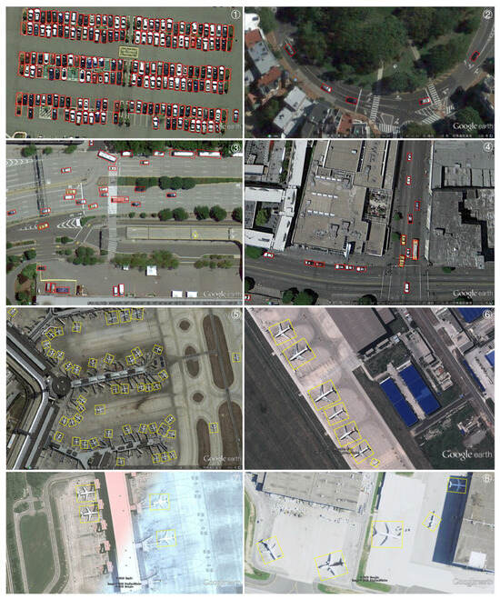
Figure 8.
Visual demonstration of the final detection results of different categories on UCAS-AOD adapting our method. To identify the location of the test results, we have marked the top right corner of each image with a circled number. Due to the high resolution of the image, please zoom in to view the test results.
As can be seen from Table 11, SSADet has the lowest floating-point arithmetic and parameter counts, while our mAP metrics rank first in Table 9 and Table 10. These fully demonstrate that our method achieves an optimal balance between computational cost and detection accuracy.
Table 11.
Comparative tests on computational metrics.
5. Conclusions and Future Work
This study presents the Staged Adaptive Alignment Detector (SAADet), which seeks to enhance the efficiency of the single-stage detector by focusing on three levels of optimization: spatial alignment, feature alignment, and task alignment. Initially, we use the SSANet backbone to extract features that match the object’s size. Afterwards, the alignment of spatial features is accomplished by employing rigorous supervision and a corrected orientated anchor to direct the alignment convergence. Ultimately, we employ the Active Rotation Kernel to separate the core features and resolve discrepancies between classification and regression. Ultimately, this strategy effectively establishes a favorable equilibrium between the detection speed and the results’ accuracy. Comprehensive testing on a pair of remote sensing datasets has confirmed the effectiveness of the proposed SAADet method. For future work, we intend to conduct further research in two aspects: first, further research on effective representations in terms of dense target distribution and large aspect ratio morphology to improve the detection accuracy, and second, considering the use of anchor-free detectors to provide more options and attempts for detecting oriented objects.
Author Contributions
Investigation, D.J.; Conceptualization, J.Z. and D.J.; Methodology, J.Z. and D.J.; Software, J.Z.; Validation, D.J.; data curation J.Z.; visualization, J.Z.; formal analysis J.Z. and D.J.; Writing—original draft, J.Z. and D.G.; Writing—review editing, J.Z. and D.G.; Supervision, D.J. and D.G. All authors have read and agreed to the published version of the manuscript.
Funding
This research is supported by the Key Laboratory of Flight Techniques and Flight Safety, CAAC, under Grant FZ2022ZZ01.
Data Availability Statement
The HRSC2016 is available at following https://sites.google.com/site/hrsc2016 (accessed on 18 May 2024). The UCAS-AOD is available at following https://github.com/Lbx2020/UCAS-AOD-dataset (accessed on 8 May 2024).
Conflicts of Interest
The authors declare no conflicts of interest.
References
- LeCun, Y.; Bengio, Y. Convolutional networks for images, speech, and time series. Handb. Brain Theory Neural Netw. 1995, 3361, 1995. [Google Scholar]
- Girshick, R.; Donahue, J.; Darrell, T.; Malik, J. Rich feature hierarchies for accurate object detection and semantic segmentation. In Proceedings of the IEEE Conference on Computer Vision and Pattern Recognition, Columbus, OH, USA, 23–28 June 2014; pp. 580–587. [Google Scholar]
- Girshick, R. Fast r-cnn. In Proceedings of the IEEE International Conference on Computer Vision, Santiago, Chile, 7–13 December 2015; pp. 1440–1448. [Google Scholar]
- Ren, S.; He, K.; Girshick, R.; Sun, J. Faster r-cnn: Towards real-time object detection with region proposal networks. Adv. Neural Inf. Process. Syst. 2015, 28, 1137–1149. [Google Scholar] [CrossRef] [PubMed]
- Dai, J.; Li, Y.; He, K.; Sun, J. R-fcn: Object detection via region-based fully convolutional networks. Adv. Neural Inf. Process. Syst. 2016, 29, 1–11. [Google Scholar]
- Lin, T.Y.; Dollár, P.; Girshick, R.; He, K.; Hariharan, B.; Belongie, S. Feature pyramid networks for object detection. In Proceedings of the IEEE Conference on Computer Vision and Pattern Recognition, Honolulu, HI, USA, 21–26 July 2017; pp. 2117–2125. [Google Scholar]
- Liu, W.; Anguelov, D.; Erhan, D.; Szegedy, C.; Reed, S.; Fu, C.Y.; Berg, A.C. Ssd: Single shot multibox detector. In Proceedings of the Computer Vision–ECCV 2016: 14th European Conference, Amsterdam, The Netherlands, 11–14 October 2016; Proceedings, Part I 14. Springer: Berlin/Heidelberg, Germany, 2016; pp. 21–37. [Google Scholar]
- Redmon, J.; Divvala, S.; Girshick, R.; Farhadi, A. You only look once: Unified, real-time object detection. In Proceedings of the IEEE Conference on Computer Vision and Pattern Recognition, Las Vegas, NV, USA, 27–30 June 2016; pp. 779–788. [Google Scholar]
- Lin, T.Y.; Goyal, P.; Girshick, R.; He, K.; Dollár, P. Focal loss for dense object detection. In Proceedings of the IEEE International Conference on Computer Vision, Venice, Italy, 22–29 October 2017; pp. 2980–2988. [Google Scholar]
- Ma, J.; Shao, W.; Ye, H.; Wang, L.; Wang, H.; Zheng, Y.; Xue, X. Arbitrary-oriented scene text detection via rotation proposals. IEEE Trans. Multimed. 2018, 20, 3111–3122. [Google Scholar] [CrossRef]
- Yang, X.; Yan, J.; Feng, Z.; He, T. R3det: Refined single-stage detector with feature refinement for rotating object. In Proceedings of the AAAI Conference on Artificial Intelligence, Virtual, 2–9 February 2021; Volume 35, pp. 3163–3171. [Google Scholar]
- Ding, J.; Xue, N.; Long, Y.; Xia, G.S.; Lu, Q. Learning RoI transformer for oriented object detection in aerial images. In Proceedings of the IEEE/CVF Conference on Computer Vision and Pattern Recognition, Long Beach, CA, USA, 15–20 June 2019; pp. 2849–2858. [Google Scholar]
- Han, J.; Ding, J.; Xue, N.; Xia, G.S. Redet: A rotation-equivariant detector for aerial object detection. In Proceedings of the IEEE/CVF Conference on Computer Vision and Pattern Recognition, Nashville, TN, USA, 20–25 June 2021; pp. 2786–2795. [Google Scholar]
- Han, J.; Ding, J.; Li, J.; Xia, G.S. Align deep features for oriented object detection. IEEE Trans. Geosci. Remote Sens. 2021, 60, 5602511. [Google Scholar] [CrossRef]
- Zhou, Y.; Ye, Q.; Qiu, Q.; Jiao, J. Oriented response networks. In Proceedings of the IEEE Conference on Computer Vision and Pattern Recognition, Honolulu, HI, USA, 21–26 July 2017; pp. 519–528. [Google Scholar]
- Cheng, G.; Zhou, P.; Han, J. Learning rotation-invariant convolutional neural networks for object detection in VHR optical remote sensing images. IEEE Trans. Geosci. Remote Sens. 2016, 54, 7405–7415. [Google Scholar] [CrossRef]
- Krizhevsky, A.; Sutskever, I.; Hinton, G.E. Imagenet classification with deep convolutional neural networks. Adv. Neural Inf. Process. Syst. 2012, 25, 1–7. [Google Scholar] [CrossRef]
- Shi, G.; Zhang, J.; Liu, J.; Zhang, C.; Zhou, C.; Yang, S. Global context-augmented objection detection in VHR optical remote sensing images. IEEE Trans. Geosci. Remote Sens. 2020, 59, 10604–10617. [Google Scholar] [CrossRef]
- Huang, H.; Huo, C.; Wei, F.; Pan, C. Rotation and scale-invariant object detector for high resolution optical remote sensing images. In Proceedings of the IGARSS 2019—2019 IEEE International Geoscience and Remote Sensing Symposium, Yokohama, Japan, 28 July–2 August 2019; pp. 1386–1389. [Google Scholar]
- Liu, Q.; Xiang, X.; Yang, Z.; Hu, Y.; Hong, Y. Arbitrary direction ship detection in remote-sensing images based on multitask learning and multiregion feature fusion. IEEE Trans. Geosci. Remote Sens. 2020, 59, 1553–1564. [Google Scholar] [CrossRef]
- Bao, S.; Zhong, X.; Zhu, R.; Zhang, X.; Li, Z.; Li, M. Single shot anchor refinement network for oriented object detection in optical remote sensing imagery. IEEE Access 2019, 7, 87150–87161. [Google Scholar] [CrossRef]
- Xiao, Z.; Wang, K.; Wan, Q.; Tan, X.; Xu, C.; Xia, F. A 2S-Det: Efficiency Anchor Matching in Aerial Image Oriented Object Detection. Remote Sens. 2020, 13, 73. [Google Scholar] [CrossRef]
- Yang, X.; Sun, H.; Sun, X.; Yan, M.; Guo, Z.; Fu, K. Position detection and direction prediction for arbitrary-oriented ships via multitask rotation region convolutional neural network. IEEE Access 2018, 6, 50839–50849. [Google Scholar] [CrossRef]
- Hua, X.; Wang, X.; Rui, T.; Zhang, H.; Wang, D. A fast self-attention cascaded network for object detection in large scene remote sensing images. Appl. Soft Comput. 2020, 94, 106495. [Google Scholar] [CrossRef]
- Zhang, G.; Lu, S.; Zhang, W. CAD-Net: A context-aware detection network for objects in remote sensing imagery. IEEE Trans. Geosci. Remote Sens. 2019, 57, 10015–10024. [Google Scholar] [CrossRef]
- Ye, X.; Xiong, F.; Lu, J.; Zhou, J.; Qian, Y. F3-Net: Feature Fusion and Filtration Network for Object Detection in Optical Remote Sensing Images. Remote Sens. 2020, 12, 4027. [Google Scholar] [CrossRef]
- Xu, C.; Li, C.; Cui, Z.; Zhang, T.; Yang, J. Hierarchical semantic propagation for object detection in remote sensing imagery. IEEE Trans. Geosci. Remote Sens. 2020, 58, 4353–4364. [Google Scholar] [CrossRef]
- Chen, L.; Liu, C.; Chang, F.; Li, S.; Nie, Z. Adaptive multi-level feature fusion and attention-based network for arbitrary-oriented object detection in remote sensing imagery. Neurocomputing 2021, 451, 67–80. [Google Scholar] [CrossRef]
- Liu, Z.; Hu, J.; Weng, L.; Yang, Y. Rotated region based CNN for ship detection. In Proceedings of the 2017 IEEE International Conference on Image Processing (ICIP), Beijing, China, 17–20 September 2017; pp. 900–904. [Google Scholar]
- Weiler, M.; Cesa, G. General e (2)-equivariant steerable cnns. Adv. Neural Inf. Process. Syst. 2019, 32, 1–13. [Google Scholar]
- Pu, Y.; Wang, Y.; Xia, Z.; Han, Y.; Wang, Y.; Gan, W.; Wang, Z.; Song, S.; Huang, G. Adaptive rotated convolution for rotated object detection. In Proceedings of the IEEE/CVF International Conference on Computer Vision, Paris, France, 2–3 October 2023; pp. 6589–6600. [Google Scholar]
- Dai, J.; Qi, H.; Xiong, Y.; Li, Y.; Zhang, G.; Hu, H.; Wei, Y. Deformable convolutional networks. In Proceedings of the IEEE International Conference on Computer Vision, Venice, Italy, 22–29 October 2017; pp. 764–773. [Google Scholar]
- Zhu, X.; Hu, H.; Lin, S.; Dai, J. Deformable convnets v2: More deformable, better results. In Proceedings of the IEEE/CVF conference on Computer Vision and Pattern Recognition, Long Beach, CA, USA, 15–20 June 2019; pp. 9308–9316. [Google Scholar]
- Jia, X.; De Brabandere, B.; Tuytelaars, T.; Gool, L.V. Dynamic filter networks. Adv. Neural Inf. Process. Syst. 2016, 29, 1–14. [Google Scholar]
- Chen, Y.; Dai, X.; Liu, M.; Chen, D.; Yuan, L.; Liu, Z. Dynamic convolution: Attention over convolution kernels. In Proceedings of the IEEE/CVF Conference on Computer Vision and Pattern Recognition, Seattle, WA, USA, 13–19 June 2020; pp. 11030–11039. [Google Scholar]
- Liu, Z.; Mao, H.; Wu, C.Y.; Feichtenhofer, C.; Darrell, T.; Xie, S. A convnet for the 2020s. In Proceedings of the IEEE/CVF Conference on Computer Vision and Pattern Recognition, New Orleans, LA, USA, 18–24 June 2022; pp. 11976–11986. [Google Scholar]
- Wang, W.; Xie, E.; Li, X.; Fan, D.P.; Song, K.; Liang, D.; Lu, T.; Luo, P.; Shao, L. Pvt v2: Improved baselines with pyramid vision transformer. Comput. Vis. Media 2022, 8, 415–424. [Google Scholar] [CrossRef]
- Guo, M.H.; Lu, C.Z.; Liu, Z.N.; Cheng, M.M.; Hu, S.M. Visual attention network. Comput. Vis. Media 2023, 9, 733–752. [Google Scholar] [CrossRef]
- Hou, Q.; Lu, C.Z.; Cheng, M.M.; Feng, J. Conv2former: A simple transformer-style convnet for visual recognition. In IEEE Transactions on Pattern Analysis and Machine Intelligence; IEEE: Piscataway, NJ, USA, 2024. [Google Scholar]
- Yu, W.; Luo, M.; Zhou, P.; Si, C.; Zhou, Y.; Wang, X.; Feng, J.; Yan, S. Metaformer is actually what you need for vision. In Proceedings of the IEEE/CVF Conference on Computer Vision and Pattern Recognition, New Orleans, LA, USA, 18–24 June 2022; pp. 10819–10829. [Google Scholar]
- Li, Y.; Hou, Q.; Zheng, Z.; Cheng, M.M.; Yang, J.; Li, X. Large selective kernel network for remote sensing object detection. In Proceedings of the IEEE/CVF International Conference on Computer Vision, Paris, France, 2–3 October 2023; pp. 16794–16805. [Google Scholar]
- Vaswani, A.; Shazeer, N.; Parmar, N.; Uszkoreit, J.; Jones, L.; Gomez, A.N.; Kaiser, Ł.; Polosukhin, I. Attention is all you need. Adv. Neural Inf. Process. Syst. 2017, 30, 1–15. [Google Scholar]
- Ding, X.; Zhang, X.; Han, J.; Ding, G. Scaling up your kernels to 31x31: Revisiting large kernel design in cnns. In Proceedings of the IEEE/CVF Conference on Computer Vision and Pattern Recognition, New Orleans, LA, USA, 18–24 June 2022; pp. 11963–11975. [Google Scholar]
- Liu, S.; Chen, T.; Chen, X.; Chen, X.; Xiao, Q.; Wu, B.; Kärkkäinen, T.; Pechenizkiy, M.; Mocanu, D.; Wang, Z. More convnets in the 2020s: Scaling up kernels beyond 51 × 51 using sparsity. arXiv 2022, arXiv:2207.03620. [Google Scholar]
- Guo, M.H.; Lu, C.Z.; Hou, Q.; Liu, Z.; Cheng, M.M.; Hu, S.M. Segnext: Rethinking convolutional attention design for semantic segmentation. Adv. Neural Inf. Process. Syst. 2022, 35, 1140–1156. [Google Scholar]
- Liu, Z.; Yuan, L.; Weng, L.; Yang, Y. A high resolution optical satellite image dataset for ship recognition and some new baselines. In Proceedings of the International conference on Pattern Recognition Applications and Methods, Porto, Portugal, 24–26 February 2017; Volume 2, pp. 324–331. [Google Scholar]
- Zhu, H.; Chen, X.; Dai, W.; Fu, K.; Ye, Q.; Jiao, J. Orientation robust object detection in aerial images using deep convolutional neural network. In Proceedings of the 2015 IEEE International Conference on Image Processing (ICIP), Quebec City, QC, Canada, 27–30 September 2015; pp. 3735–3739. [Google Scholar]
- Li, X.; Wang, W.; Hu, X.; Yang, J. Selective kernel networks. In Proceedings of the IEEE/CVF Conference on Computer Vision and Pattern Recognition, Long Beach, CA, USA, 15–20 June 2019; pp. 510–519. [Google Scholar]
- Jiang, Y.; Zhu, X.; Wang, X.; Yang, S.; Li, W.; Wang, H.; Fu, P.; Luo, Z. R2CNN: Rotational region CNN for orientation robust scene text detection. arXiv 2017, arXiv:1706.09579. [Google Scholar]
- Xiao, Z.; Qian, L.; Shao, W.; Tan, X.; Wang, K. Axis learning for orientated objects detection in aerial images. Remote Sens. 2020, 12, 908. [Google Scholar] [CrossRef]
- Feng, P.; Lin, Y.; Guan, J.; He, G.; Shi, H.; Chambers, J. TOSO: Student’sT distribution aided one-stage orientation target detection in remote sensing images. In Proceedings of the ICASSP 2020—2020 IEEE International Conference on Acoustics, Speech and Signal Processing (ICASSP), Virtual, 4–9 May 2020; pp. 4057–4061. [Google Scholar]
- Liao, M.; Zhu, Z.; Shi, B.; Xia, G.s.; Bai, X. Rotation-sensitive regression for oriented scene text detection. In Proceedings of the IEEE Conference on Computer Vision and Pattern Recognition, Salt Lake City, UT, USA, 18–23 June 2018; pp. 5909–5918. [Google Scholar]
- Qian, W.; Yang, X.; Peng, S.; Yan, J.; Guo, Y. Learning modulated loss for rotated object detection. In Proceedings of the AAAI Conference on Artificial Intelligence, Vancouver, BC, Canada, 20–27 February 2021; Volume 35, pp. 2458–2466. [Google Scholar]
- Xu, Y.; Fu, M.; Wang, Q.; Wang, Y.; Chen, K.; Xia, G.S.; Bai, X. Gliding vertex on the horizontal bounding box for multi-oriented object detection. IEEE Trans. Pattern Anal. Mach. Intell. 2020, 43, 1452–1459. [Google Scholar] [CrossRef]
- Song, Q.; Yang, F.; Yang, L.; Liu, C.; Hu, M.; Xia, L. Learning point-guided localization for detection in remote sensing images. IEEE J. Sel. Top. Appl. Earth Obs. Remote Sens. 2020, 14, 1084–1094. [Google Scholar] [CrossRef]
- Yi, J.; Wu, P.; Liu, B.; Huang, Q.; Qu, H.; Metaxas, D. Oriented object detection in aerial images with box boundary-aware vectors. In Proceedings of the IEEE/CVF Winter Conference on Applications of Computer Vision, Virtual, 5–9 January 2021; pp. 2150–2159. [Google Scholar]
- Pan, X.; Ren, Y.; Sheng, K.; Dong, W.; Yuan, H.; Guo, X.; Ma, C.; Xu, C. Dynamic refinement network for oriented and densely packed object detection. In Proceedings of the IEEE/CVF Conference on Computer Vision and Pattern Recognition, Seattle, WA, USA, 13–19 June 2020; pp. 11207–11216. [Google Scholar]
- Ming, Q.; Zhou, Z.; Miao, L.; Zhang, H.; Li, L. Dynamic anchor learning for arbitrary-oriented object detection. In Proceedings of the AAAI Conference on Artificial Intelligence, Virtual, 2–9 February 2021; Volume 35, pp. 2355–2363. [Google Scholar]
- Ming, Q.; Miao, L.; Zhou, Z.; Yang, X.; Dong, Y. Optimization for arbitrary-oriented object detection via representation invariance loss. IEEE Geosci. Remote Sens. Lett. 2021, 19, 8021505. [Google Scholar] [CrossRef]
- Yang, X.; Hou, L.; Zhou, Y.; Wang, W.; Yan, J. Dense label encoding for boundary discontinuity free rotation detection. In Proceedings of the IEEE/CVF Conference on Computer Vision and Pattern Recognition, Nashville, TN, USA, 20–25 June 2021; pp. 15819–15829. [Google Scholar]
- Ming, Q.; Miao, L.; Zhou, Z.; Song, J.; Yang, X. Sparse label assignment for oriented object detection in aerial images. Remote Sens. 2021, 13, 2664. [Google Scholar] [CrossRef]
- Yang, X.; Yan, J. On the arbitrary-oriented object detection: Classification based approaches revisited. Int. J. Comput. Vis. 2022, 130, 1340–1365. [Google Scholar] [CrossRef]
- Ming, Q.; Miao, L.; Zhou, Z.; Dong, Y. CFC-Net: A critical feature capturing network for arbitrary-oriented object detection in remote-sensing images. IEEE Trans. Geosci. Remote Sens. 2021, 60, 5605814. [Google Scholar] [CrossRef]
- Yang, X.; Yan, J.; Ming, Q.; Wang, W.; Zhang, X.; Tian, Q. Rethinking rotated object detection with gaussian wasserstein distance loss. In Proceedings of the International Conference on Machine Learning, PMLR, Virtual, 18–24 July 2021; pp. 11830–11841. [Google Scholar]
- Ming, Q.; Miao, L.; Zhou, Z.; Song, J.; Dong, Y.; Yang, X. Task interleaving and orientation estimation for high-precision oriented object detection in aerial images. Isprs J. Photogramm. Remote Sens. 2023, 196, 241–255. [Google Scholar] [CrossRef]
- Redmon, J.; Farhadi, A. Yolov3: An incremental improvement. arXiv 2018, arXiv:1804.02767. [Google Scholar]
- Xia, G.S.; Bai, X.; Ding, J.; Zhu, Z.; Belongie, S.; Luo, J.; Datcu, M.; Pelillo, M.; Zhang, L. DOTA: A large-scale dataset for object detection in aerial images. In Proceedings of the IEEE Conference on Computer Vision and Pattern Recognition, Salt Lake City, UT, USA, 18–23 June 2018; pp. 3974–3983. [Google Scholar]
Disclaimer/Publisher’s Note: The statements, opinions and data contained in all publications are solely those of the individual author(s) and contributor(s) and not of MDPI and/or the editor(s). MDPI and/or the editor(s) disclaim responsibility for any injury to people or property resulting from any ideas, methods, instructions or products referred to in the content. |
© 2024 by the authors. Licensee MDPI, Basel, Switzerland. This article is an open access article distributed under the terms and conditions of the Creative Commons Attribution (CC BY) license (https://creativecommons.org/licenses/by/4.0/).