Estimation of Hub Center Loads for Individual Pitch Control for Wind Turbines Based on Tower Loads and Machine Learning

Abstract

In wind turbines, to investigate the cause of failures and evaluate the remaining lifetime, it may be necessary to measure their loads. However, it is often difficult to do so with only strain gauges in terms of cost and time, so a method to evaluate loads by utilizing only simple measurements is quite useful. In this study, we investigated a method with machine learning to estimate hub center loads, which is important in terms of preventing damage to equipment inside the nacelle. Traditionally, measuring hub center loads requires performing complex strain measurements on rotating parts, such as the blades or the main shaft. On the other hand, the tower is a stationary body, so the strain measurement difficulty is relatively low. We tackled the problem as follows: First, machine learning models that predict the time history of hub center loads from the tower top loads and operating condition data were developed by using aeroelastic analysis. Next, the accuracy of the model was verified by using measurement data from an actual wind turbine. Finally, individual pitch control, which is one of the applications of the time history of hub center loads, was performed using aeroelastic analysis, and the load reduction effect with the model prediction values was equivalent to that of the conventional method.

1. Introduction

To preserve the ecosystem on Earth, global warming must be urgently suppressed. One of the important solutions to this problem is to make the power sector, which produces a significant amount of CO₂, carbon-free. Wind power generation is one of the most successful renewable energy processes and has matured technologically, but further expansion and cost reduction are expected. Accordingly, progress is being made in making wind turbines even larger, developing floating wind turbines that can be installed in deeper waters, applying wind power generation technology to complex terrain, etc. This requires the development of new technologies and application to new environments, but real-world implementation is often hindered by complications [1,2].

In investigating the cause of wind turbine failure, it is important to understand the loads acting on the target parts at the site. The loads applied to a wind turbine are evaluated with a simulator during the turbine design process [3] and are verified by measuring strain on a demonstration wind turbine installed on essentially flat terrain on land [4]. However, wind turbines are installed in the natural environment, and the conditions vary considerably depending on the installation location. Therefore, to confirm the loads on a malfunctioning wind turbine, it is necessary to carry out measurements on the malfunctioning turbine itself. In addition, determining the loads at the installation site can aid in the optimization of operation, the evaluation of the remaining lifetime, lifetime extension decisions, maintenance planning, etc.

Load and stress evaluation at the installation site of a wind turbine is generally performed by measuring strain near the target area, which is highly accurate. However, when it is necessary to do so on multiple wind turbines for remaining lifetime evaluation or the investigation of the cause of a malfunction, it is not realistic in terms of costs and labor to perform strain measurement on all the target wind turbines. To overcome these financial and manpower drawbacks, technologies have been developed to evaluate the target loads and stress by using other data acquired from the wind turbine. Machine learning models were trained to predict the main fatigue loads of wind turbines based on SCADA data, which are collected for all wind turbines and include operating conditions and nacelle acceleration [5]. In addition, SCADA 10 min data generally have many variables due to parameters and statistical methods, but using all these data as inputs for a machine learning model would cause overfitting issues and poor insights/analysis; therefore, effective feature selection and dimensionality reduction methods were examined [6,7,8]. In addition, a method was proposed to use the strain data for a limited period as training data for model learning, and the necessary period was investigated [9].

Fatigue is often a deciding factor in the design of support structures for offshore wind turbines, and load monitoring is required. Noppe et al. [10] developed a method to evaluate the loads of offshore wind turbine support structures by evaluating quasi-static loads from 1 Hz SCADA data and dynamic loads from tower acceleration data. Santos et al. [11] showed that adding tower acceleration and wave data in addition to SCADA data allows for a more accurate assessment of lateral fatigue, where damage is greater in XL monopiles. Santos et al. [12] also attempted to estimate the wind turbine foundation fatigue load of an entire wind farm from a limited number of wind turbine strain data and found that it was possible to predict it with an MAE of 1% for the training turbine and an MAE of less than 3% for other turbines. Santos et al. [13] also developed a model that incorporates physical laws into a neural network to improve accuracy in life expectancy prediction and enable safety evaluation.

Regarding blade fatigue prediction techniques, evaluation methods using only 10 min SCADA values have been studied; methods [14] that reproduce fast fluctuations through simulation and create a database and methods [15] that incorporate Variational Auto-Encoder (VAE), a deep learning technique, have been proposed. In the prediction of component fatigue, a physics-informed neural network method [16] has been proposed for main bearings; it uses physical laws for cyclic fatigue, for which the theory is generally established, and a neural network with wind speed and temperature as inputs for grease lubrication, to which mathematical formulas are difficult to apply. Regarding the internal loads of drivetrain bearings, which are difficult to measure, a method [17] called virtual sensor has been proposed in which a machine learning model is developed from the analysis results by using measurable inputs such as acceleration.

Attempts have also been made to use data other than the commonly used strain and acceleration data. Methods have been developed to track blade movement from inertial measurement and navigation algorithms [18] and to estimate static loads on towers by using satellite data [19]. A model has been developed to predict the fatigue loads of a wind turbine that is subjected to the wake of an adjacent wind turbine based on the load measurements of the latter [20].

Most load prediction methods focus on fatigue loads, but a model has been proposed in which the proximity of the random forest model is used to predict extreme loads in each tower section based on tower acceleration and other parameters [21].

As described above, methods have been developed to predict the loads and stress on a target by combining other data with machine learning models without directly measuring strain. However, there are few techniques to predict hub center loads, which is important for preventing equipment failures inside the nacelle, except for an example [22] in which the thrust force was predicted based on strain at the tower bottom. Furthermore, although many techniques have been developed to predict statistical values, such as damage equivalent load (hereinafter referred to as “DEL”), there are few examples of evaluating the time history of loads [23]. Therefore, in this study, with the aim of evaluating the time history of hub center loads, the target wind turbine was selected (Section 2), the parameters that could be evaluated were identified, and an effective machine learning model was examined (Section 3). Next, a machine learning model was developed by using aeroelastic analysis (Section 4) and was then validated by using measured data from the actual wind turbine (Section 5). Application in individual pitch control [24], which is one of the benefits of determining the time history of hub center loads, was also examined (Section 6), and finally, conclusions were drawn (Section 7).

2. Wind Turbine and Target Loads

The target wind turbine is presented in Section 2.1, the loads to be evaluated are shown in Section 2.2, and the strain measurements made on the prototype are described in Section 2.3.

2.1. Wind Turbine

The target was a downwind 2 MW wind turbine manufactured by Hitachi, Ltd. (Tokyo, Japan).

Table 1. Wind turbine general specifications.

Manufacturer	Hitachi, Ltd.
Model	HTW2.0-86
Rotor diameter	86 m
Rotor position	Downwind
Rated power	2 MW
Number of blades	3
Tilt angle	−8 deg
Corning angle	5 deg
Hub height	78 m
Power control	Pitch, variable speed

shows its general specifications.

2.2. Target Loads

The targets of the evaluation were the loads in the hub coordinate system [25] (hereinafter referred to as “hub center loads”), which are important for the design of equipment in the nacelle. Figure 1 shows the main components of a wind turbine and the coordinate system at each wind turbine location. The hub coordinate system does not rotate with the rotor and has the hub center as its origin. Here, the x-axis direction is the rotor axis direction, the z-axis direction is perpendicular to the x-axis and points upward, and the y-axis direction is horizontal. In this study, we focused on the most important hub center loads: rotational torque (hereinafter referred to as “MXN”), nodding moment (hereinafter referred to as “MYN”), yawing moment (hereinafter referred to as “MZN”), and thrust force (hereinafter referred to as “FXN”). The loads were normalized by using the respective design extreme loads (the maximum of the absolute values of the maximum and minimum).

2.3. Load Measurement

The measurement data used to validate the predictive model in Section 5 were acquired in March 2015 from a prototype wind turbine located along the coast of Tainai City, Niigata Prefecture, Japan. Figure 1 shows the measurement points at the blade root and at the tower top. The blades were measured at four points in each axis direction on a cross-section 1.35 m from the root of the three blades, but the edge direction was measured at points shifted 22.5 deg from the axial direction to avoid the over lamination area. At the tower top, measurements were taken at four points at 90 deg intervals on a cross-section 1.0 m below the tower top. At two of those points, in addition to the vertical direction for bending moment measurement, the ±45 deg directions were measured for torque measurement with biaxial gages.

The measurement system is shown in Figure 2, and the instruments and sensors are shown in

Table 2. Instruments and sensors.

Instrument/Sensor	Model (Manufacturer)	Specifications
Instrument 1	ENV-1030-CAN (Moog Insensys)	Range: ±3000 με (min.) Resolution: 2 με (typ.) Accuracy: 5 με (short-term)
Optical strain gage	Composite retrofit blade sensor array set (Moog Insensys)	-
Instrument 2	NTB-500A, NTB-50A (Kyowa electronic instruments)	Range: ±30,000 με Resolution: 0.1 με Accuracy: 0.1%RD
Electrical strain gage	KFG-5-350-C1-11 L15C2R KFG-5-350-D16-11 L15C2S (Kyowa electronic instruments)	-
Instrument 3	NTB-500A, NTB-51A (Kyowa electronic instruments)	Range: 10V Resolution: 100 μV Accuracy: 0.1%RD

. While general electrical strain gages were used to measure the tower, fiber optic strain gages were used to measure the blades, which are highly resistant to environmental conditions such as lightning strikes. Basically, wired CAN communication was used for data transmission, but existing optical fiber communication was used for transmission from the nacelle to the tower bottom. Strain at the blade root, strain at the tower top, and wind turbine operating conditions output from the wind turbine controller were integrated into a PC installed at the tower bottom, where they were synchronously measured, and data were stored.

3. Explanatory Variables and Machine Learning Models

In this section, variables that can be used in the evaluation of the target loads are discussed in Section 3.1, and effective machine learning models are discussed in Section 3.2.

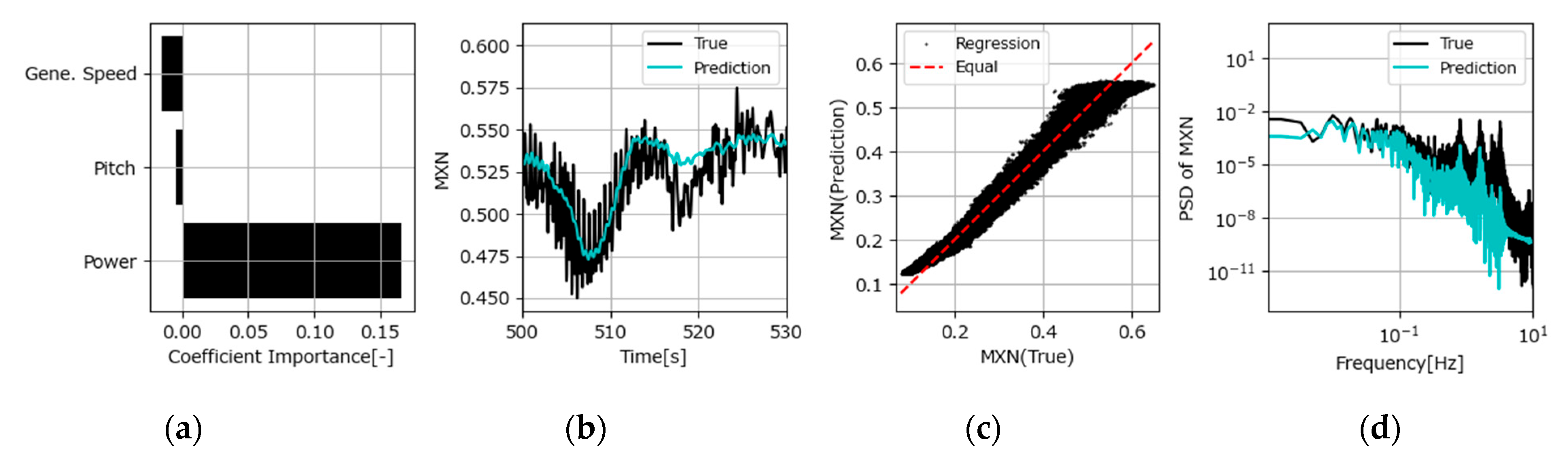
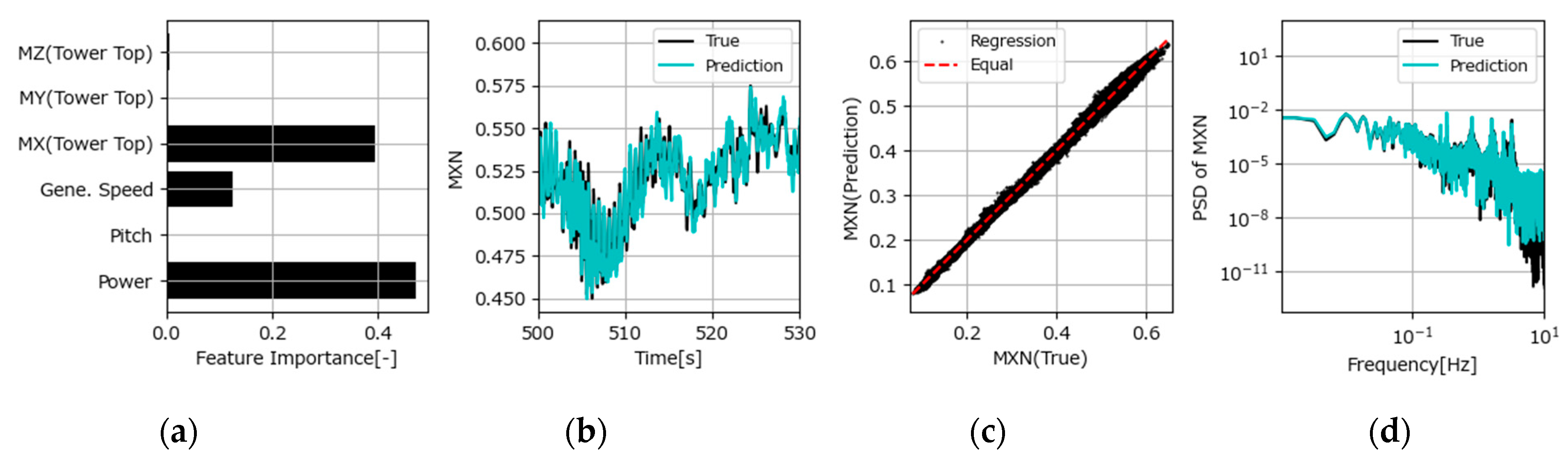
3.1. Explanatory Variables

To determine parameters with which to predict hub center loads, the correlations among hub center loads, main loads, and wind turbine behavior were investigated. The Pearson correlation coefficient was used as an index of correlation, with a value closer to 1 indicating a positive correlation, a value closer to −1, a negative correlation, and a value of 0 no correlation. For the evaluation, 10 min data from an aeroelastic analysis at an average wind speed of 14 m/s were used. The DataFrame.corr function of the Pandas library in the Python programming language was used for the analysis.

The Pearson correlation coefficients for the hub center loads (MXN, MYN, MZN, and FXN), the wind and operating conditions commonly obtained with SCADA (wind speed, power, yaw misalignment, pitch angle, and azimuth angle), and the main loads (moments at blade root, tower top, and tower bottom) are shown in Figure 3. The correlation coefficients with absolute values greater than 0.9 were none for MXN, tower top MY for MYN, tower top MZ and tower bottom MZ for MZN, and pitch angle and tower bottom MY for FXN. Blade root MY did not have a high correlation on its own, but when combined with azimuth and pitch angles, the hub center loads could be predicted.

Next, the correlations between hub center loads and nacelle behaviors are shown in Figure 4. The correlation coefficients with absolute values greater than 0.9 were none for MXN and MYN, yaw displacement for MZN, and fore–aft displacement and nod angle for FXN. While strain measurement is necessary to determine the loads shown in Figure 3, nacelle behavior may be more easily determined by using accelerometers, gyroscopes, inclinometers, GPS, etc.

3.2. Machine Learning Model

There are various models for machine learning. As reported in this section, we examined analysis accuracy and training time. Here, neural networks were excluded. Pycaret, a Python wrapper, was used for this study.

Table 3. Performance of machine learning models.

Model	MAE	MSE	RMSE	R2	RMSLE	MAPE	TT (s)
Extra Trees Regressor	0.0077	0.0001	0.011	0.98	0.0095	0.32	0.98
CatBoost Regressor	0.0081	0.0001	0.011	0.98	0.0098	0.32	1.76
Random Forest Regressor	0.0117	0.0003	0.017	0.95	0.0140	0.50	2.56
K Neighbors Regressor	0.0126	0.0003	0.017	0.95	0.0146	0.44	0.47
Extreme Gradient Boosting	0.0130	0.0003	0.017	0.95	0.0151	0.41	0.83
Light Gradient Boosting Machine	0.0139	0.0004	0.019	0.94	0.0160	0.53	0.59
Decision Tree Regressor	0.0196	0.0009	0.030	0.84	0.0247	0.68	0.52
Gradient Boosting Regressor	0.0302	0.0015	0.039	0.73	0.0306	1.61	1.17
AdaBoost Regressor	0.0509	0.0039	0.063	0.31	0.0514	1.99	0.62
Ridge Regression	0.0579	0.0053	0.073	0.06	0.0580	3.05	0.46
Linear Regression	0.0590	0.0055	0.074	0.03	0.0589	3.11	0.98
Lasso Least Angle Regression	0.0590	0.0055	0.074	0.03	0.0589	3.12	0.46
Lasso Regression	0.0590	0.0055	0.074	0.03	0.0589	3.12	0.47
Elastic Net	0.0590	0.0055	0.074	0.03	0.0589	3.12	0.47
Huber Regressor	0.0592	0.0055	0.075	0.02	0.0591	3.14	0.47
Orthogonal Matching Pursuit	0.0593	0.0056	0.075	0.02	0.0591	3.15	0.46
Dummy Regressor	0.0602	0.0057	0.075	0.00	0.0598	3.22	0.64
Passive Aggressive Regressor	0.0604	0.0058	0.076	−0.01	0.0607	3.04	0.46
Least Angle Regression	0.0614	0.0060	0.077	−0.06	0.0622	3.08	0.48
Bayesian Ridge	0.2656	0.2139	0.328	−35.11	0.1945	8.05	0.45

shows the evaluation results of each machine learning model when the objective variable is MYN, the explanatory variables are three operating conditions (power, pitch angle, and generator speed) and six-blade root section bending moments, and 10 min data from the aeroelastic analysis at an average wind speed of 14 m/s are used. Here, the evaluation indices are mean absolute error (MAE), mean squared error (MSE), root mean squared error (RMSE), coefficient of determination (R²), log mean squared error (RMSLE), mean absolute percentage error (MAPE), and training time (TT).

Models that use ensemble learning of decision trees rank highly. This is thought to be because of the nonlinear behavior that output and rotational speed are limited to a rated value, and the pitch angle is only adjusted when energy above a certain level is input, which decision trees are excellent at reproducing. In this study, we used a nonlinear model called Extra Tree Regressor (hereinafter referred to as “ET”), which combines decision trees and ensemble learning using bagging to provide a good balance between analysis accuracy and analysis time, and a linear model called Linear Regression (hereinafter referred to as “LR”), which is simple and makes results easy to interpret.

4. Predictive Model Development

In this section, we attempt to establish a method to predict the hub center loads using machine learning models with relatively simple measurement parameters by aeroelastic analysis. The analysis flow is shown in Section 4.1, and the evaluation results of the model’s predictive accuracy are shown in Section 4.2.

4.1. Analysis Flow

The data used were the results of an analysis conducted by using Bladed aeroelastic analysis software [26]. The input wind conditions for the aeroelastic analysis are shown in

Table 4. Wind parameter values for aeroelastic simulation.

Parameter	Values
Mean wind speed [m/s]	8, 14
Turbulence intensity (Iref) [−]	0.12, 0.14, 0.16, 0.18
Wind shear exponent (α) [−]	0.14, 0.2, 0.33, 0.5
Turbulent seed [−]	1~6

. The average wind speed was set to 8 m/s for optimal efficiency operation and 14 m/s for rated output operation. A total of 192 cases were analyzed for 10 min each and an output period of 0.04 s, with two average wind speeds, four turbulence intensities, four wind shear values, and six turbulent seeds.

The flow of developing a machine learning model is shown in Figure 5. Here, the aeroelastic analysis results were divided into a training dataset and a test dataset, but rather than dividing all the data randomly, the cases with turbulent seeds 1 to 4 were used as the training dataset (128 cases), and the cases with turbulent seeds 5 and 6 were used as the test dataset (64 cases). This is because when the data for the same analysis case are divided into training and test datasets, the data for adjacent times are very similar and not completely independent, and there is a risk of overestimating prediction accuracy due to data leakage.

4.2. Model Evaluation

Two machine learning models were used: Linear Regression (LR) and Extra Trees Regressor (ET), which are discussed in Section 3.2. The set of explanatory variables was set in four ways, as shown in

Table 5. Explanatory variable sets.

	Parameter	Number
Pr1	Power, pitch angle, and generator speed	3
Pr2	Power, pitch angle, generator speed, nacelle acceleration X, Y, and Z	6
Pr3	Power, pitch angle, generator speed, tower bottom MX, MY, and MZ	6
Pr4	Power, pitch angle, generator speed, tower top MX, MY, and MZ	6

, based on the study presented in Section 3.1. Here, Pr1 consists of variables normally used in wind turbine control and does not require additional sensors. Pr2 is P1 plus the three directional nacelle accelerations that are standardly measured. Pr3 is Pr1 plus three moments at the tower bottom, and Pr4 is Pr1 plus three moments at the tower top. Pr3 and Pr4 require strain measurements at the tower, but it is easier to measure the strain at the tower because it is not a rotating part, compared with strain measurements at the blades or hub, which is generally performed when evaluating hub center loads.

For the analytical accuracy of the prediction model, the coefficients of determination (R²) are shown in Figure 6, and the ratios of the predicted value of damage equivalent load (DEL) to the true value when the slope (m) of the SN curve is 10 (hereinafter referred to as “m = 10”) are shown in Figure 7. DEL is the fatigue load expressed as a scalar quantity and calculated by Equation (1).

$$DEL={\left({\displaystyle \frac{\sum n_i{S_i}^m}{n_{ref}}}\right)}^{1/m}$$

(1)

where $S_i$ is the load of i-th range bin of the fatigue load spectrum, $n_i$ is the number of cycles in the i-th range bin of the fatigue load spectrum, and $n_{ref}$ is the reference number of load cycles. MXN LR results show that the DEL ratio can be small even when R² is close to 1, so caution is required. The results of Pr1, Pr2, and Pr3 for MXN and FXN show that changing the machine learning model from LR to ET improves the analysis accuracy of DEL. On the other hand, MYN Pr4 has high analytical accuracy with LR but slightly lower with ET, so ET is not necessarily superior. FXN is below 0.95 for all models and indices, so if higher prediction accuracy is required, it is necessary to consider changing the explanatory variables, etc. While MYN requires the inclusion of loads at the tower top to improve the analysis accuracy, MZN has high prediction accuracy even with loads at the tower bottom, so the variables to be obtained depend on the target load.

The variable importance, time history, correlation, and frequency distribution for each prediction model are shown in Figure 8, Figure 9, Figure 10, Figure 11, Figure 12, Figure 13, Figure 14, Figure 15, Figure 16, Figure 17, Figure 18, Figure 19, Figure 20, Figure 21, Figure 22 and Figure 23. Here, only Pr1 and Pr4 are displayed as explanatory variable sets. Pr1 is the case using only common operation conditions, and Pr4 is the case that was shown to work well. Variable importance is defined differently depending on the machine learning model: coefficient importance for LR is the proportionality constant multiplied by the standard deviation, and feature importance for ET is the reduced contribution of Gini impurity; however, both are indicators of the importance of each explanatory variable to the prediction.

For the prediction of MXN (Figure 8, Figure 9, Figure 10 and Figure 11), the linear model LR using operating conditions Pr1 (Figure 8) can predict slow fluctuations due to the contribution of the output but not fast fluctuations. When the nonlinear model ET is used (Figure 9), fast fluctuations are also predicted, but the oscillation phases are not aligned. By adding the tower top loads to the explanatory variables (Figure 10 and Figure 11), we can also predict fast fluctuations due to the contribution of tower top MX.

For FXN prediction (Figure 12, Figure 13, Figure 14 and Figure 15), even the linear model LR using operating conditions Pr1 (Figure 12) can predict slow fluctuations due to the contributions of pitch angle, power, and generator speed but cannot predict fast fluctuations. When the nonlinear model ET is used (Figure 13), the prediction accuracy of fast fluctuations improves, but the phases are not aligned. Adding the tower top loads to the explanatory variables (Figure 14 and Figure 15) slightly improves the prediction accuracy due to the contribution of tower top MX, but not significantly.

For MYN prediction (Figure 16, Figure 17, Figure 18 and Figure 19), the linear model LR using operating conditions Pr1 (Figure 16) outputs almost constant values and cannot be predicted. When the nonlinear model ET is used (Figure 17), the fast fluctuation component is included, but the oscillation phase is not correct. Adding the tower top loads to the explanatory variables (Figure 18 and Figure 19) improves the prediction accuracy due to the contribution of tower top MY, and both slow and fast fluctuations are generally predicted. However, in the case of the nonlinear model ET (Figure 19), the prediction is not accurate when the true value is large, and this may be because the training dataset does not contain such large values.

MZN prediction (Figure 20, Figure 21, Figure 22 and Figure 23) was almost the same as MYN prediction.

From the above, it was found that MXN, FXN, MYN, and MZN are generally predictable for both linear and nonlinear machine learning models when a set of explanatory variables are operating conditions and tower top loads. It should be noted, however, that FXN has slightly lower prediction accuracy.

5. Predictive Model Validation

As presented in this section, the predictive models of hub center loads developed in Section 4 were validated by using measured data from the actual wind turbine. The validation method is shown in Section 5.1, and the results in Section 5.2.

5.1. Validation Flow

The verification flow is shown in Figure 24. By using the strain measured at the blade root, the blade loads were calculated, and by combining them with the pitch angle and azimuth angle data, the measured hub center loads were calculated and used as the true values. On the other hand, the tower top loads were calculated by using the strain measured at the tower top and the nacelle direction angle, and the three operating conditions were added to them as explanatory variables; finally, the hub center loads were calculated by using the linear (LR) or nonlinear (ET) machine learning model developed as shown in Section 4 and used as the predicted values.

Only MYN and MZN were evaluated as hub center loads. This is because it is difficult to derive MXN and FXN from blade loads; further, determining MYN and MZN is particularly important for preventing damage to equipment in the nacelle, and prediction techniques for them are not well established.

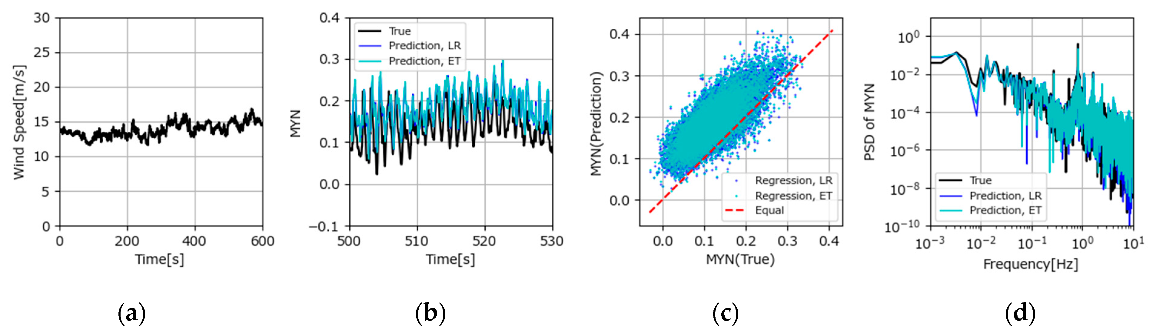
5.2. Validation Results

The data used were 10 min data with average wind speeds of approximately 7, 14, and 22 m/s. The first two values (7 and 14 m/s) were selected because they were close to the wind speeds (8 and 14 m/s) used for the development of the machine learning model, and a wind speed (22 m/s) that deviated from them was further selected.

Comparisons of true and predicted MYN values are shown in Figure 25, Figure 26 and Figure 27, and MZN comparisons are shown in Figure 28, Figure 29 and Figure 30. The predicted average values are slightly larger than the true values at the wind speeds of 7 and 14 m/s, but the fluctuation components are generally consistent in both amplitude and phase. Predictions are generally equivalent to whether the machine learning model is linear (LR) or nonlinear (ET).

The coefficient of determination R² and the DEL (m = 10) ratios for the true and predicted values are shown in

Table 6. Validation results.

		R2			DEL (m = 10) Ratio
		7 m/s	14 m/s	22 m/s	7 m/s	14 m/s	22 m/s
MYN	LR	−1.752	−0.841	0.626	0.905	1.024	0.983
	ET	−2.081	−0.992	0.627	0.937	1.032	0.952
MZN	LR	0.217	0.039	0.553	0.807	0.999	0.778
	ET	0.173	0.106	0.541	0.839	1.011	0.787

. R² was lower for both MYN and MZN, especially at 7 and 14 m/s, suggesting that the effect of the shifted mean was significant. The error for DEL (m = 10) was within 10% for MYN, while for some data for MZN, it was over 20%. As for the cause of the lower prediction accuracy for MZN compared with MYN, the measurement accuracy of tower top MZ, which contributes the most to the prediction of MZN, was suspected to be responsible since the analysis in Section 4 did not show such a trend. In the measurement of tower top MZ, strain gauges are installed at +45 degrees and −45 degrees from the vertical, and their values are subtracted to eliminate the bending effect, but there are some difficulties, such as the introduction of bending effects if the installation angle is off.

6. Individual Pitch Control

The advantage of obtaining the time history of the hub center loads is that it can be used for individual pitch control (hereinafter referred to as “IPC”) in addition to load evaluation. Normally, blade strain is often measured in the implementation of IPC, but the blade where the sensor is installed and the hub where the measurement device is installed are rotating bodies, so there is a risk of damage, and communications using a slip ring or wireless connection have the risk of communication failure. On the other hand, the method established in Section 4 is more reliable because it can be measured on a stationary tower. As reported in this section, the performance of IPC with the tower top loads was verified with simulation. The evaluation method is shown in Section 6.1, and the evaluation results are in Section 6.2.

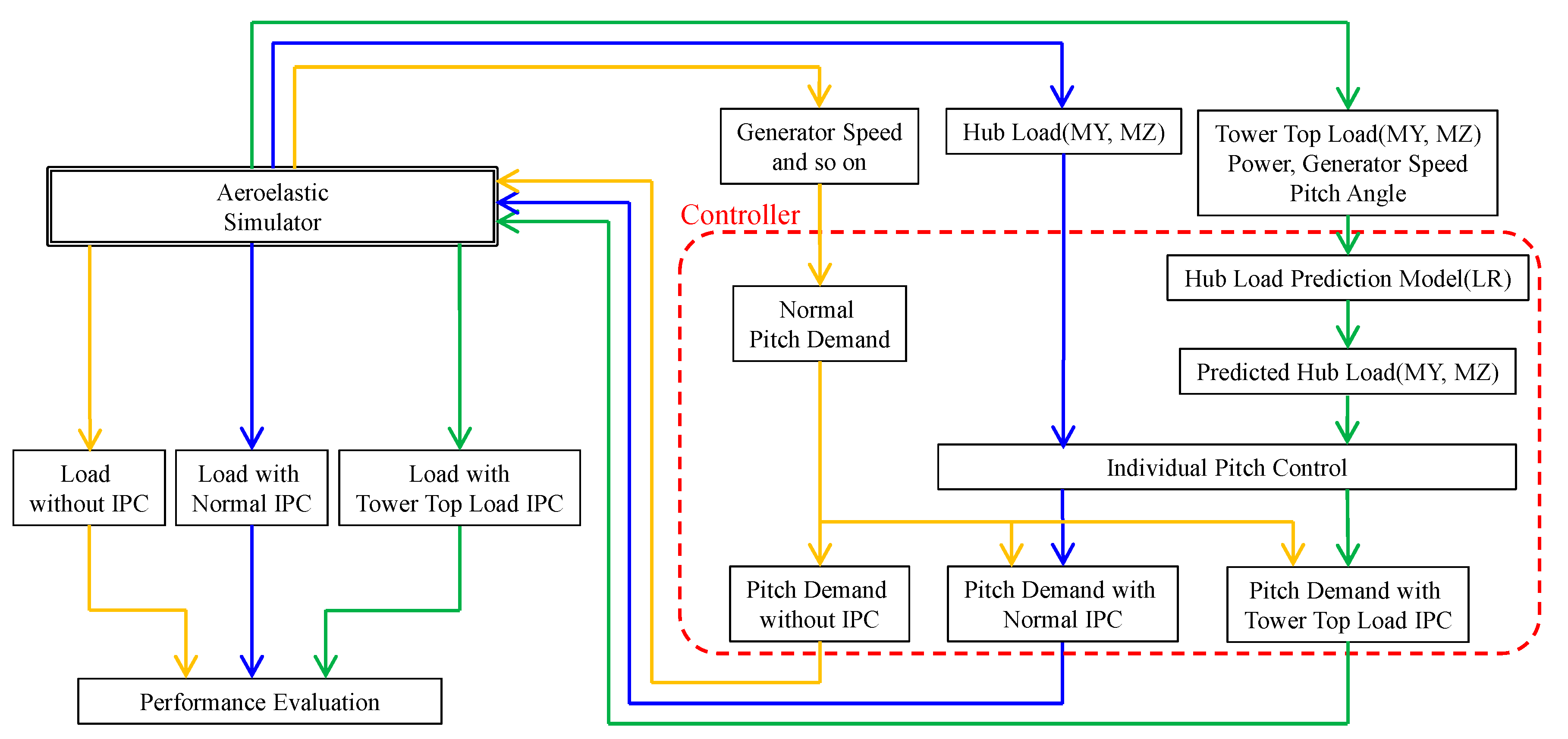
6.1. Evaluation Flow

The performance evaluation flow of IPC is shown in Figure 31. Three controllers were prepared for the simulation. The first one was a controller without IPC, the second one a controller that implements general IPC based on MYN and MZN, and the third one a controller that predicts the hub center loads by using a machine learning model with tower top loads and operating conditions as inputs (see Section 4) and implements IPC based on the predicted loads. Here, due to software constraints, only MY and MZ were input as tower top loads, and MX was not used. However, since the contribution of tower top load MX to the prediction of MYN and MZN is small (see Figure 18 and Figure 22), the impact is minor. For the machine learning model, we used the easy-to-implement Linear Regression (LR) model because there was no significant difference in prediction accuracy between linear and nonlinear models when the tower top loads were used (see Section 4 and Section 5). The performance of IPC with the tower top loads was evaluated by performing an aeroelastic analysis on the three controllers and comparing the results. IPC was carried out according to Equation (2).

$$\left(\begin{array}{c}{\beta }_1\\ {\beta }_2\\ {\beta }_3\end{array}\right)=\left(\begin{array}{c}\cos \left(\theta +{\theta }_{cor}\right)\\ \cos \left(\theta +{\theta }_{cor}+2\pi /3\right)\\ \cos \left(\theta +{\theta }_{cor}+4\pi /3\right)\end{array}\right. \left.\begin{array}{c}\sin \left(\theta +{\theta }_{cor}\right)\\ \sin \left(\theta +{\theta }_{cor}+2\pi /3\right)\\ \sin \left(\theta +{\theta }_{cor}+4\pi /3\right)\end{array}\right)\left(\begin{array}{c}{PI}_{MYN}\\ {PI}_{MZN}\end{array}\right)$$

(2)

where ${\beta }_1$, ${\beta }_2$, and ${\beta }_3$ are the pitch demands for pitches 1, 2, and 3 by IPC, $\theta$ is the rotor azimuth angle, ${\theta }_{cor}$ is the rotor azimuth correction angle, and ${PI}_{MYN}$ and ${PI}_{MZN}$ are the results of PI control for MYN and MZN.

6.2. Evaluation Results

For the aeroelastic analysis, three input winds with different turbulent seeds were prepared for average wind speeds of 8, 12, 16, 20, and 24 m/s, and the analysis was performed for 10 min for each. The results of the evaluation for blade root MY, MYN, and MZN with the DEL (m = 10) are shown in Figure 32. No significant effect of IPC was seen in MYN or MZN, but a significant effect was seen in blade root MY at high wind speeds above 16 m/s. This is an effect for a wind turbine with a rated power of 2 MW and a rotor diameter of 86 m, which is relatively small for today’s wind turbines, and a larger effect can be expected for larger wind turbines due to the large variation in wind speed on the rotor plane. IPC with the tower top loads was shown to be as effective as general IPC with hub center loads, indicating the potential of IPC with tower top loads.

7. Conclusions

In this study, we developed a method for predicting the time history of hub center loads, which is important for investigating equipment failures in the nacelle, by combining simple measurement and machine learning. We also performed IPC using the predicted values. The main results obtained from this study are described as follows:

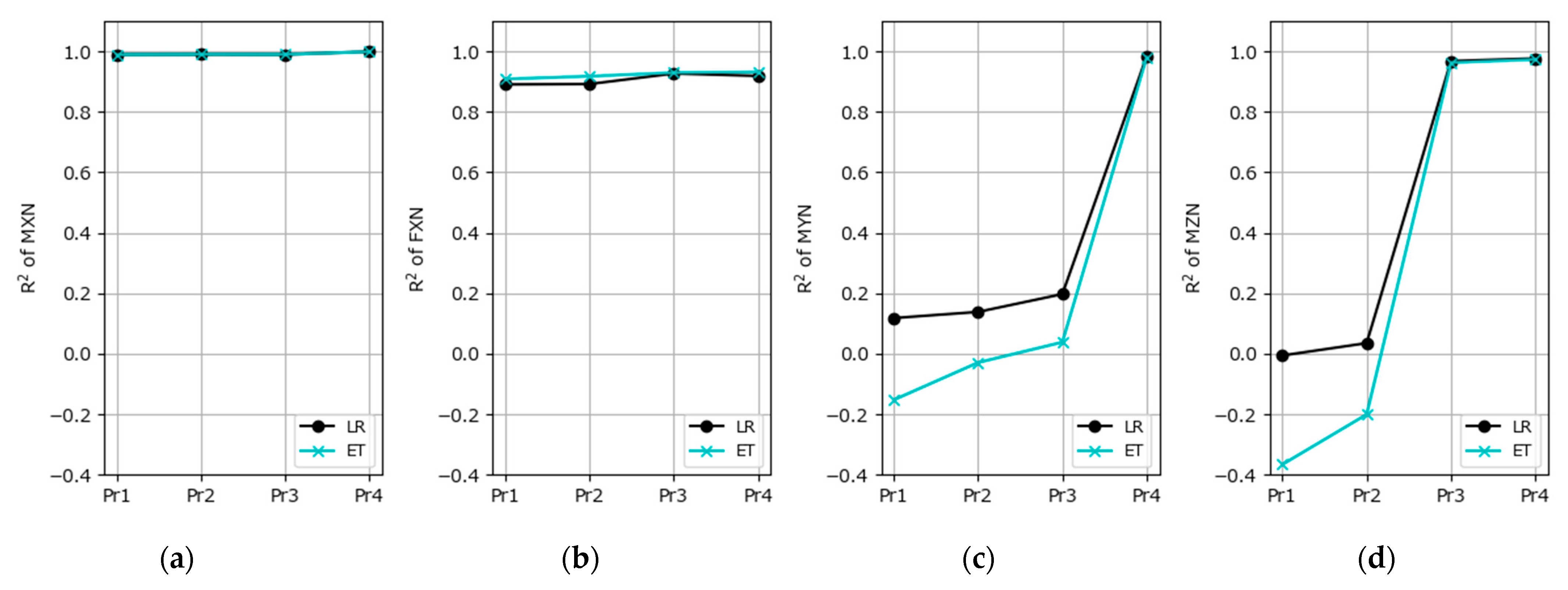
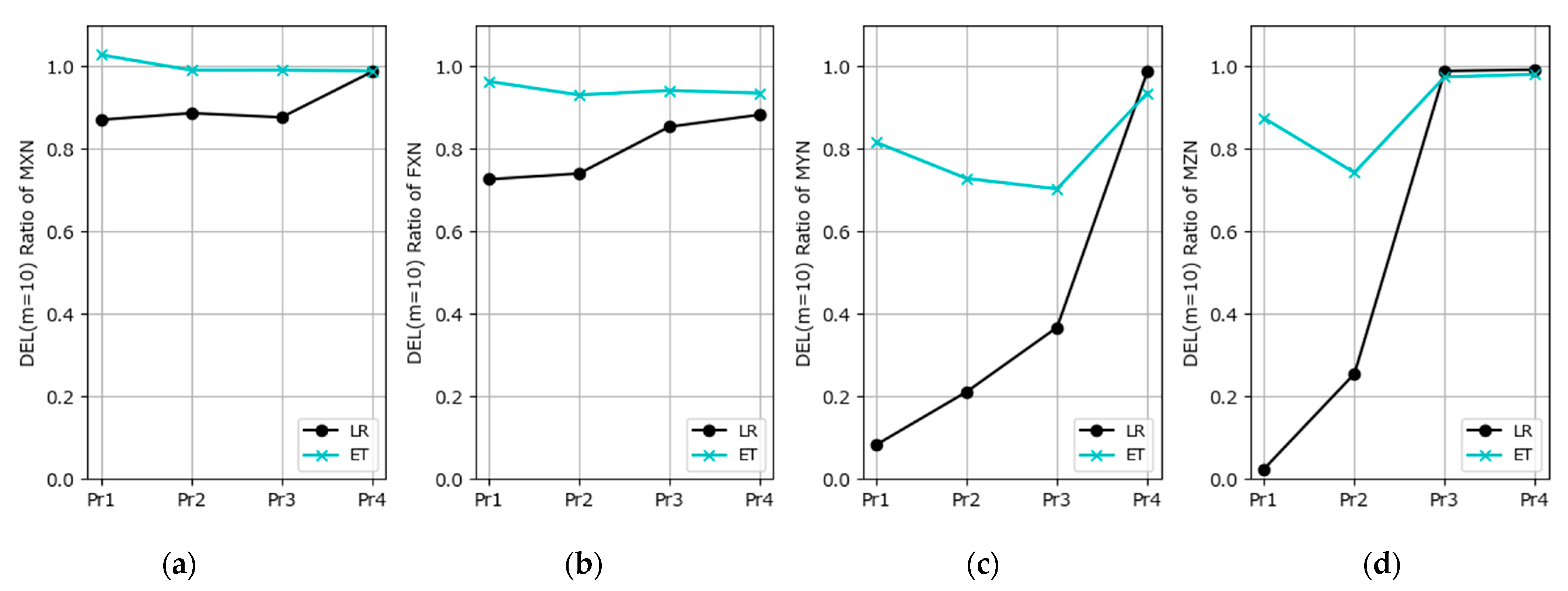
• When a linear machine learning model is insufficient for predicting MXN and FXN, a nonlinear machine learning model can improve the prediction accuracy.
• In predicting MXN, MYN, and MZN, the linear machine learning model provides sufficient prediction accuracy when tower top loads are added to the set of explanatory variables.
• In the prediction of FXN, when operating conditions, nacelle accelerations, tower top loads, and tower bottom loads are used as explanatory variables, there is a DEL error of more than 5%, even with a nonlinear machine learning model.
• While MYN prediction requires tower top loads, MYN can be predicted with tower bottom loads, so the explanatory variables required depend on the target load.
• The prediction models for MYN and MZN developed from the aeroelastic analysis based on tower top loads and operating conditions as explanatory variables were validated by using measured data, and the DEL (m = 10) errors were within 10% for MYN and within 23% for MZN.
• The time history of the hub center loads was predicted by a machine learning model with tower top loads and operating conditions as explanatory variables, and IPC was implemented by using these loads. The results show that the load reduction effect was equivalent to that of general IPC based on hub loads.

As future developments of this research study, the following are planned:

• Investigate whether analysis accuracy can be improved when a neural network is used as a machine learning model.
• Examine whether hub loads can be predicted from the behaviors of the nacelle.

References

1. Uchida, T.; Takakuwa, S. A Large-Eddy Simulation-Based Assessment of the Risk of Wind Turbine Failures Due to Terrain-Induced Turbulence over a Wind Farm in Complex Terrain. Energies 2019, 12, 1925. [Google Scholar] [CrossRef]
2. Chou, J.-S.; Chiu, C.-K.; Huang, I.-K.; Chi, K.-N. Failure analysis of wind turbine blade under critical wind loads. Eng. Fail. Anal. 2013, 27, 99–118. [Google Scholar] [CrossRef]
3. IEC 61400-1; Wind Turbines Part 1: Design Requirement. International Electrotechnical Commission: Geneva, Switzerland, 2005.
4. IEC 61400-13; Wind Turbines Part 13: Measurement of Mechanical Loads. International Electrotechnical Commission: Geneva, Switzerland, 2001.
5. Cosack, N.; Kühn, M. An Approach for Fatigue Load Monitoring without Load Measurement Devices. In Proceedings of the European Wind Energy Conference, Marseille, France, 16–19 March 2009. [Google Scholar]
6. Vera-Tudela, L.; Kühn, M. On the selection of input variables for a wind turbine load monitoring system. Procedia Technol. 2014, 15, 726–736. [Google Scholar] [CrossRef]
7. Movsessian, A.; Schedat, M.; Faber, T. Modelling tower fatigue loads of a wind turbine using data mining techniques on SCADA data. Wind Energy Sci. Discuss. 2020, 2020, 1–20. [Google Scholar]
8. Movsessian, A.; Schedat, M.; Faber, T. Feature selection techniques for modelling tower fatigue loads of a wind turbine with neural networks. Wind. Energy Sci. 2021, 6, 539–554. [Google Scholar] [CrossRef]
9. Seifert, J.; Vera-Tudela, L.; Kuhna, M. Training requirements of a neural network used for fatigue load estimation of offshore wind turbines. Energy Procedia 2017, 137, 315–322. [Google Scholar] [CrossRef]
10. Noppe, N.; Iliopoulos, A.; Weijtjens, W.; Devriendt, C. Full load estimation of an offshore wind turbine based on SCADA and accelerometer data. J. Phys. Conf. Ser. 2016, 753, 072025. [Google Scholar] [CrossRef]
11. Santos, F.D.N.; Noppe, N.; Weijtjens, W.; Devriendt, C. Data-driven farm-wide fatigue estimation on jacket-foundation OWTs for multiple SHM setups. Wind Energ. Sci. 2022, 7, 299–321. [Google Scholar] [CrossRef]
12. Santos, F.D.N.; Noppe, N.; Weijtjens, W.; Devriendt, C. Results of fatigue measurement campaign on XL monopiles and early predictive models. J. Phys. Conf. Ser. 2022, 2265, 032092. [Google Scholar] [CrossRef]
13. de N Santos, F.; D’Antuono, P.; Robbelein, K.; Noppe, N.; Weijtjens, W.; Devriendt, C. Long-term fatigue estimation on offshore wind turbines interface loads through loss function physics-guided learning of neural networks. Renew. Energy 2023, 205, 461–474. [Google Scholar] [CrossRef]
14. Chrétien, A.; Tahan, A.; Cambron, P.; Oliveira-Filho, A. Operational Wind Turbine Blade Damage Evaluation Based on 10-min SCADA and 1 Hz Data. Energies 2023, 16, 3156. [Google Scholar] [CrossRef]
15. Mylonas, C.; Abdallah, I.; Chatzi, E. Conditional variational autoencoders for probabilistic wind turbine blade fatigue estimation using Supervisory, Control, and Data Acquisition data. Wind Energy 2021, 24, 1122–1139. [Google Scholar] [CrossRef]
16. Yucesan, Y.A.; Viana, F.A.C. Wind Turbine Main Bearing Fatigue Life Estimation with Physics-informed Neural Networks. In Proceedings of the Annual Conference of the PHM Society, Scottsdale, AZ, USA, 21–26 September 2019; pp. 1–14. [Google Scholar]
17. Kamel, O.; Kretschmer, M.; Pfeifer, S.; Luhmann, B.; Hauptmann, S.; Bottasso, C.L. Data-driven virtual sensor for online loads estimation of drivetrain of wind turbines. Forsch. Ingenieurwesen/Eng. Res. 2023, 87, 31–38. [Google Scholar] [CrossRef]
18. Avenda, L.D.; Abdallah, I.; Chatzi, E. Virtual fatigue diagnostics of wake-affected wind turbine via Gaussian Process Regression. Renew. Energy 2021, 170, 539–561. [Google Scholar]
19. Wiens, M.; Martin, T.; Meyer, T.; Zuga, A. Reconstruction of operating loads in wind turbines with inertial measurement units. Forsch. Ingenieurwesen 2021, 85, 181–188. [Google Scholar] [CrossRef]
20. Wei, D.; Li, D.; Jiang, T.; Lyu, P.; Song, X. Load identification of a 2.5 MW wind turbine tower using Kalman filtering techniques and BDS data. Eng. Struct. 2023, 281, 115763. [Google Scholar] [CrossRef]
21. Nielsen, M.S.; Rohde, V. A surrogate model for estimating extreme tower loads on wind turbines based on random forest proximities. J. Appl. Stat. 2022, 49, 485–497. [Google Scholar] [CrossRef] [PubMed]
22. Noppe, N.; Weijtjens, W.; Devriendt, C. Modeling of quasi-static thrust load of wind turbines based on 1 s SCADA data. Wind Energ. Sci. 2018, 3, 139–147. [Google Scholar] [CrossRef]
23. Pandit, R.; Astolfi, D.; Hong, J.; Infield, D.; Santos, M. SCADA data for wind turbine data-driven condition/performance monitoring: A review on state-of-art, challenges and future trends. Wind Eng. 2023, 47, 422–441. [Google Scholar] [CrossRef]
24. Bossanyi, E.A. Individual blade pitch control for load reduction. Wind Energy 2003, 6, 119–128. [Google Scholar] [CrossRef]
25. Germanischer Lloyd. Guideline for the Certification of Wind Turbine; Germanischer Lloyd: Hamburg, Germany, 2010. [Google Scholar]
26. GL Garrad Hassan. Bladed Version 4.2.0.83; GL Garrad Hassan: Bristol, UK, 2012. [Google Scholar]
Figure 1. Coordinate systems and measurement points.
Electronics 13 03648 g001
Figure 2. Measurement system.
Electronics 13 03648 g002
Figure 3. Pearson correlation coefficients for hub loads, wind and operating conditions, and main loads.
Electronics 13 03648 g003
Figure 4. Pearson correlation coefficients for hub loads and nacelle behaviors.
Electronics 13 03648 g004
Figure 5. Analysis flow for machine learning model development.
Electronics 13 03648 g005
Figure 6. Model accuracy: R2 of (a) MXN; (b) FXN; (c) MYN; (d) MZN.
Electronics 13 03648 g006
Figure 7. Model accuracy: DEL (m = 10) ratios of (a) MXN, (b) FXN, (c) MYN, and (d) MZN.
Electronics 13 03648 g007
Figure 8. LR model prediction of MXN using input feature set Pr1: (a) Coefficient importance. (b) Time history. (c) Correlation. (d) Frequency distribution.
Electronics 13 03648 g008
Figure 9. ET model prediction of MXN using input feature set Pr1: (a) Feature importance. (b) Time history. (c) Correlation. (d) Frequency distribution.
Electronics 13 03648 g009
Figure 10. LR model prediction of MXN using input feature set Pr4: (a) Coefficient importance. (b) Time history. (c) Correlation. (d) Frequency distribution.
Electronics 13 03648 g010
Figure 11. ET model prediction of MXN using input feature set Pr4: (a) Feature importance. (b) Time history. (c) Correlation. (d) Frequency distribution.
Electronics 13 03648 g011
Figure 12. LR model prediction of FXN using input feature set Pr1: (a) Coefficient importance. (b) Time history. (c) Correlation. (d) Frequency distribution.
Electronics 13 03648 g012
Figure 13. ET model prediction of FXN using input feature set Pr1: (a) Feature importance. (b) Time history. (c) Correlation. (d) Frequency distribution.
Electronics 13 03648 g013
Figure 14. LR model prediction of FXN using input feature set Pr4: (a) Coefficient importance. (b) Time history. (c) Correlation. (d) Frequency distribution.
Electronics 13 03648 g014
Figure 15. ET model prediction of FXN using input feature set Pr4: (a) Feature importance. (b) Time history. (c) Correlation. (d) Frequency distribution.
Electronics 13 03648 g015
Figure 16. LR model prediction of MYN using input feature set Pr1: (a) Coefficient importance. (b) Time history. (c) Correlation. (d) Frequency distribution.
Electronics 13 03648 g016
Figure 17. ET model prediction of MYN using input feature set Pr1: (a) Feature importance. (b) Time history. (c) Correlation. (d) Frequency distribution.
Electronics 13 03648 g017
Figure 18. LR model prediction of MYN using input feature set Pr4: (a) Coefficient importance. (b) Time history. (c) Correlation. (d) Frequency distribution.
Electronics 13 03648 g018
Figure 19. ET model prediction of MYN using input feature set Pr4: (a) Feature importance. (b) Time history. (c) Correlation. (d) Frequency distribution.
Electronics 13 03648 g019
Figure 20. LR model prediction of MZN using input feature set Pr1: (a) Coefficient importance. (b) Time history. (c) Correlation. (d) Frequency distribution.
Electronics 13 03648 g020
Figure 21. ET model prediction of MZN using input feature set Pr1: (a) Feature importance. (b) Time history. (c) Correlation. (d) Frequency distribution.
Electronics 13 03648 g021
Figure 22. LR model prediction of MZN using input feature set Pr4: (a) Coefficient importance. (b) Time history. (c) Correlation. (d) Frequency distribution.
Electronics 13 03648 g022
Figure 23. ET model prediction pf MZN using input feature set Pr4: (a) Feature importance. (b) Time history. (c) Correlation. (d) Frequency distribution.
Electronics 13 03648 g023
Figure 24. Model validation flow.
Electronics 13 03648 g024
Figure 25. Validation of MYN prediction models at wind speeds of 7 m/s: (a) Wind speed time history. (b) Load time history. (c) Correlation. (d) Frequency distribution.
Electronics 13 03648 g025
Figure 26. Validation of MYN prediction models at wind speeds of 14 m/s: (a) Wind speed time history. (b) Load time history. (c) Correlation. (d) Frequency distribution.
Electronics 13 03648 g026
Figure 27. Validation of MYN prediction models at wind speeds of 22 m/s: (a) Wind speed time history. (b) Load time history. (c) Correlation. (d) Frequency distribution.
Electronics 13 03648 g027
Figure 28. Validation of MZN prediction models at wind speeds of 7 m/s: (a) Wind speed time history. (b) Load time history. (c) Correlation. (d) Frequency distribution.
Electronics 13 03648 g028
Figure 29. Validation of MZN prediction models at wind speeds of 14 m/s: (a) Wind speed time history. (b) Load time history. (c) Correlation. (d) Frequency distribution.
Electronics 13 03648 g029
Figure 30. Validation of MZN prediction models at wind speeds of 22 m/s: (a) Wind speed time history. (b) Load time history. (c) Correlation. (d) Frequency distribution.
Electronics 13 03648 g030
Figure 31. IPC performance evaluation flow.
Electronics 13 03648 g031
Figure 32. IPC performance evaluation results: (a) blade root MY; (b) MYN; (c) MZN.
Electronics 13 03648 g032