A Novel Short-Term PM_2.5 Forecasting Approach Using Secondary Decomposition and a Hybrid Deep Learning Model

Abstract

PM_2.5 pollution poses an important threat to the atmospheric environment and human health. To precisely forecast PM_2.5 concentration, this study presents an innovative combined model: EMD-SE-GWO-VMD-ZCR-CNN-LSTM. First, empirical mode decomposition (EMD) is used to decompose PM_2.5, and sample entropy (SE) is used to assess the subsequence complexity. Secondly, the hyperparameters of variational mode decomposition (VMD) are optimized by Gray Wolf Optimization (GWO) algorithm, and the complex subsequences are decomposed twice. Next, the sequences are divided into high-frequency and low-frequency parts by using the zero crossing rate (ZCR); the high-frequency sequences are predicted by a convolutional neural network (CNN), and the low-frequency sequences are predicted by a long short-term memory network (LSTM). Finally, the predicted values of the high-frequency and low-frequency sequences are reconstructed to obtain the final results. The experiment was conducted based on the data of 1009A, 1010A, and 1011A from three air quality monitoring stations in the Beijing area. The results indicate that the R² value of the designed model increased by 2.63%, 0.59%, and 1.88% on average in the three air quality monitoring stations, respectively, compared with the other single model and the mixed model, which verified the significant advantages of the proposed model.

1. Introduction

As the world’s population grows faster and more urbanized, more pollutants are released into the atmosphere than it can naturally absorb, leading to a growing problem with air pollution [1,2,3]. The primary measure of air pollution, PM_2.5, has a significant effect on air quality [4]. Particulate matter in the air with a diameter of less than or equal to 2.5 μm is referred to as PM_2.5, which is mainly generated from the combustion of fossil fuels, industrial production, transportation, and other processes of waste gas and smoke. It mainly comes from exhaust gases and soot produced during fossil fuel combustion, industrial production, transportation, and other processes [5].

PM_2.5 has a significant impact on both the ecological environment and human health. Firstly, PM_2.5 reduces atmospheric visibility, leading to the formation of haze weather, which severely affects urban landscapes and residents’ quality of life [6]. Secondly, PM_2.5 poses a serious threat to human health. These fine particles can penetrate deep into the lungs and even pass through lung alveolar walls into the bloodstream, causing serious damage to the respiratory and cardiovascular systems [7]. According to reports from the World Health Organization, millions of people worldwide die prematurely each year due to exposure to PM_2.5 pollution. Specific data indicate that for every increase of 10 µg/m³ in PM_2.5 concentration, there is an approximately 6% increase in cardiovascular disease mortality and an approximately 8% increase in lung cancer mortality [8]. Additionally, PM_2.5 is closely associated with increased incidence of respiratory diseases such as childhood asthma and chronic obstructive pulmonary disease [9]. Therefore, accurate prediction of PM_2.5 concentration is crucial for public health protection and environmental policy-making. Through effective forecasting, governments can issue timely air quality alerts, implement corresponding emission reduction measures, and mitigate the impact of pollution on public health. To facilitate understanding,

Table 1. Abbreviations and their full forms in this study.

Abbreviation	Full Form
ARIMA	Auto Regressive Moving Average
SARIMA	Seasonal Auto Regressive Moving Average
GRA	Grey Relational Analysis
SVR	Support Vector Regression
CNN	Convolutional Neural Network
1D-CNN	One-Dimensional Convolutional Neural Network
RNN	Recurrent Neural Network
LSTM	Long Short-Term Memory Network
NLSTM	Nested Long Short-Term Memory Network
BiLSTM	Bidirectional Long Short-Term Memory Network
LSSVM	Least-Squares Support Vector Machine
WT	Wavelet Transform
SAE	Stacked Autoencoder
EWT	Empirical Wavelet Transform
ESWT	Extended Stationary Wavelet Transform
EMD	Empirical Mode Decomposition
CEEMDAN	Complete Ensemble Empirical Mode Decomposition with Adaptive Noise
VMD	Variational Mode Decomposition
SA	Self-Attention
SE	Sample Entropy
AQI	Air Quality Index
ICA	Imperial Competition Algorithm
ESN	Echo State Network
GWO	Gray Wolf Optimizer
EAG	Exponential Adaptive Gradient
IMF	Intrinsic Mode Function
mRMR	Minimum Redundancy Maximum Relevance
GWNN	Geographically Weighted Neural Network
WOA	Whale Optimization Algorithm
ELM	Extreme Learning Machine

lists the commonly used abbreviations and their corresponding full forms in this manuscript.

A time series prediction issue relying on past series data to infer future numerical trends is PM_2.5 concentration prediction [10]. Current PM_2.5 concentration prediction models primarily encompass the following: physical models, statistical models, machine learning models, deep learning models, and hybrid models. Physical models are based on atmospheric physical, chemical, and kinetic equations, taking into account meteorological conditions, atmospheric dispersion, and chemical reactions to predict PM_2.5 concentrations. Commonly used physical models include CMAQ [11], WRF-Chem [12,13], and CAMS [14]. However, physical models are more complex to construct and require more knowledge of the environment and chemistry. On the other hand, statistical models are straightforward in theory and do not require sophisticated knowledge. Statistical models used for PM_2.5 concentration prediction mainly include auto regressive moving average model (ARIMA) [15], seasonal auto regressive moving average model (SARIMA) [16], and grey relational analysis (GRA) [17]. Due to the limitations of statistical models in capturing complex nonlinear relationships, the introduction of machine learning models can better address these challenges. Mainstream machine learning models mainly include Decision Tree [18], Random Forest [19], and support vector regression (SVR) [20]. As data size and complexity increase, machine learning models have limitations in dealing with more complex nonlinear relationships, thus driving the rise of deep learning models. Deep learning models for time series prediction mainly include convolutional neural networks (CNNs) [21], long short-term memory (LSTM) [22], and Transformer models [23]. Some researchers have started looking into hybrid models [24,25] to further lower the error of PM_2.5 prediction by combining the benefits of various models.

Several academics have suggested using signal decomposition techniques to reduce the non-stationary nature of PM_2.5 sequences and improve the models’ forecasting accuracy, as this has an effect on modeling accuracy. Qiao et al. [26] used the wavelet transform (WT) to decompose PM_2.5 sequences and used stacked auto encoder (SAE) and LSTM to make predictions. However, the wavelet basis function that is selected has a direct impact on the WT’s performance, and choosing a different wavelet basis function could have different consequences for signal feature extraction. Kim et al. [27] used the empirical wavelet transform (EWT) and CNN combined with a bidirectional long- and short-term memory neural network (BiLSTM) to forecast PM_2.5 levels. Although EWT is a data adaptive wavelet transform method that does not require pre-selection of wavelet basis functions and successfully overcomes the limitations of traditional wavelet transforms, empirical mode decomposition (EMD) performs better in capturing the local features and nonlinear oscillations of the signal. Yuan et al. [28] designed a self-attention mechanism (SA), and EMD and used LSTM to forecast the classroom’s PM_2.5 concentration. They used EMD to decompose the original PM_2.5 sequence and adopted an improved SA mechanism to reconstruct the subsequence. The reconstructed subsequence was input into LSTM for prediction. It greatly increased the accuracy of the prediction. Consequently, in this research, the original PM_2.5 sequences were decomposed using EMD, and the complexity of each subsequence was assessed using sample entropy (SE).

In pursuit of heightened prediction accuracy, certain scholars utilize secondary decomposition techniques to delve deeper into extracting data characteristics. Yang et al. [29] delved into secondary decomposition through the integration of complete ensemble empirical modal decomposition (CEEMDAN) and variational modal decomposition (VMD) with the least-squares support vector machine (LSSVM) to forecast PM_2.5 concentration. The findings illustrated the superior predictive accuracy of this model compared to both single and hybrid models. Liu et al. [30] used EWT-SE-VMD to decompose the original air quality index (AQI) sequence into multiple subsequences, used the imperial competition algorithm (ICA) to select the subsequences and input them into the echo state network (ESN) for prediction, and output the future AQI. While VMD offers superior advantages in mathematical stability and addressing local extreme point problems, the manual configuration of the number of decomposition layers and penalty factor can influence its effectiveness. To address this issue, the Gray Wolf Optimizer (GWO) algorithm, requiring fewer parameters and devoid of the necessity for gradient information, is employed in this study to fine-tune the parameters of VMD.

Researchers have used different models for PM_2.5 concentration prediction. Ragab et al. [31] used a one-dimensional deep convolutional neural network (1D-CNN) combined with exponential adaptive gradient (EAG) optimization to predict the air pollution index in Malaysia, but the 1D-CNN struggles with capturing long-term dependencies. Kristiani et al. [32] utilized the LSTM deep learning technique for short-term PM_2.5 concentration forecasting, resulting in significantly enhanced predictive performance. The efficacy of an individual model is constrained, and superior outcomes can be attained through the fusion of diverse network architectures. Ding et al. [33] devised a hybrid deep learning model that integrates both CNN and LSTM architectures to forecast PM_2.5 concentration, resulting in high accuracy. Nonetheless, in the majority of their research, the impact of both high and low data frequency on the prediction outcomes was overlooked. Therefore, in this study, ZCR is employed to separate the data’s high and low frequencies. The long-term features of the low-frequency sequences are extracted using LSTM, and the local features of the high-frequency sequences are extracted using CNN, to accomplish the prediction of the concentration of PM_2.5 by more thoroughly capturing the various aspects of the sequential data. This study’s main innovations and contributions are as follows:

(1)

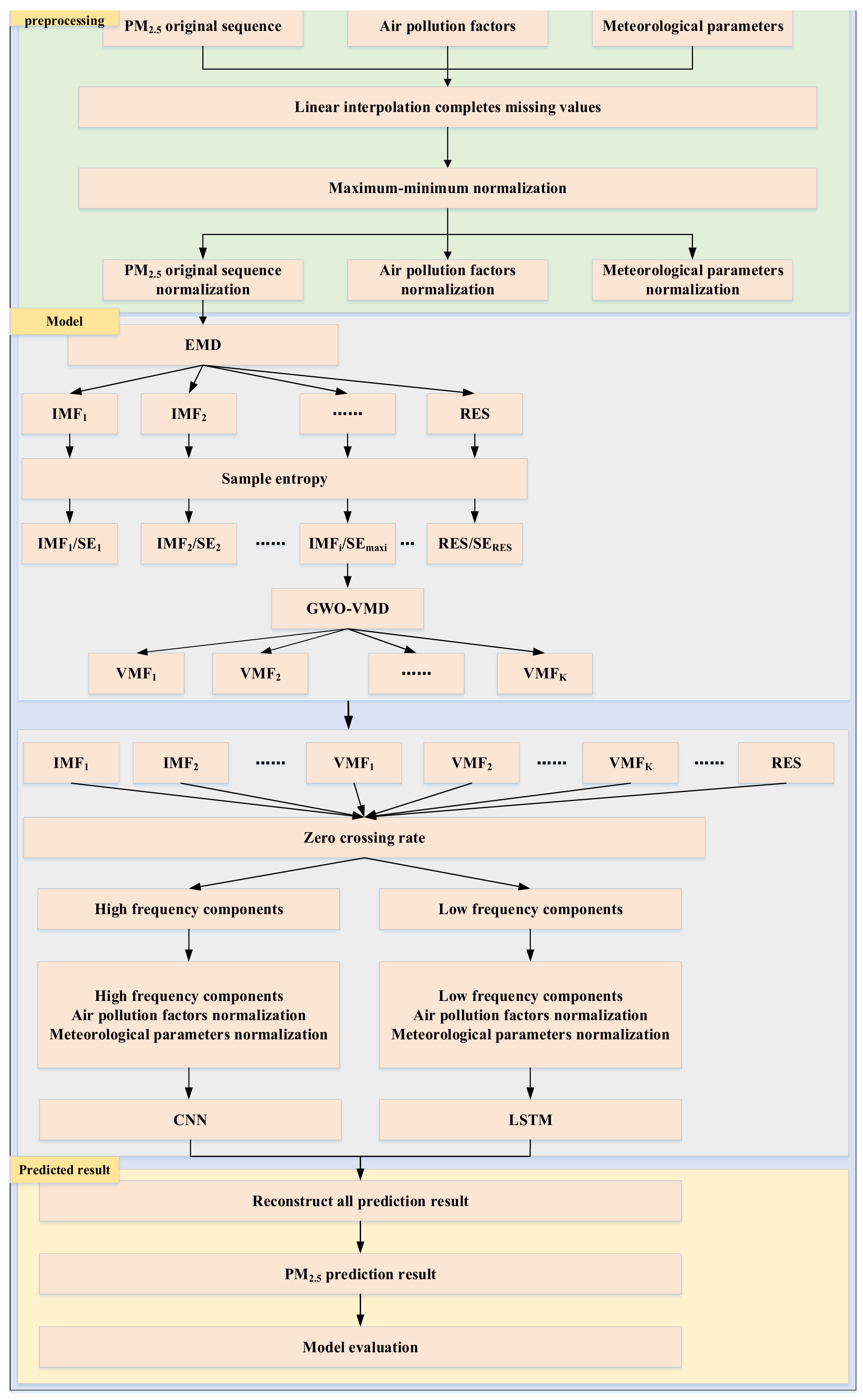
An innovative quadratic decomposition method, EMD-SE-GWO-VMD, is proposed. This method can more accurately extract the intrinsic non-stationary characteristics and periodic variation trend when decomposing PM_2.5 series and significantly improve the performance of the prediction model.

(2)

Taking into account the impact of high-frequency and low-frequency sequences on PM_2.5 concentration prediction, the ZCR-CNN-LSTM method is proposed. This method effectively distinguishes and processes the high-frequency and low-frequency components in the data, reducing information confusion. Simultaneously, it comprehensively captures and utilizes the temporal characteristics and periodicity of the data, significantly enhancing the precision of PM_2.5 concentration forecast.

(3)

An inventive hybrid model, hybrid EMD-SE-GWO-VMD-ZCR-CNN-LSTM, is further designed for the short-term prediction of PM_2.5 based on (1) and (2). The model makes full use of the non-stationarity and periodicity of PM_2.5 data, effectively solves the influence of high- and low-frequency series on PM_2.5 prediction, and significantly improves the reliability of PM_2.5 prediction.

(4)

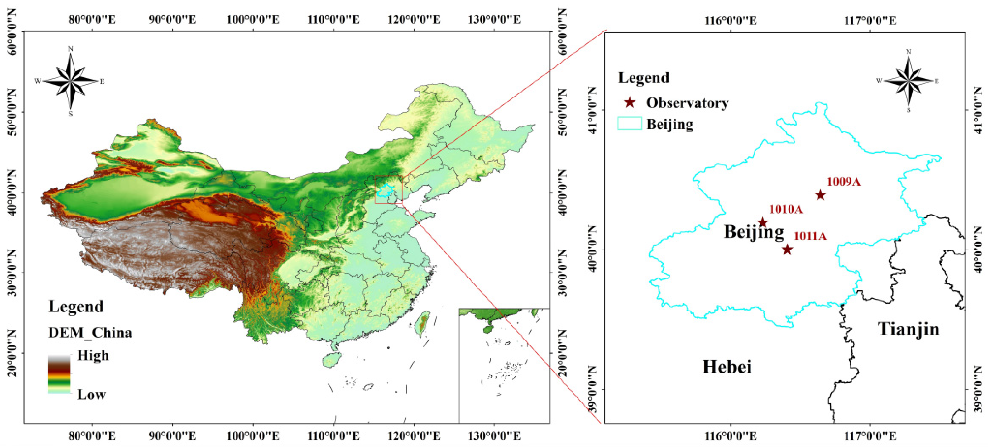
In order to evaluate the effectiveness and stability of the model, a series of novel experiments are designed. Data from three air quality monitoring stations 1009A, 1010A, and 1011A in the Beijing area are used. Comparing experimental outcomes with different prediction models, the R² of this model at the three air quality monitoring stations increases by an average of 2.63%, 0.59%, and 1.88%, respectively. This demonstrates that the model has a major benefit in terms of increasing the precision of PM_2.5 concentration forecast.

2. Data and Methods

2.1. Description of the Dataset

As the capital of China, Beijing is not only the political, cultural, and economic center but also faces complex air quality challenges. The city is densely populated and highly urbanized. Its location in the northern part of the North China Plain subjects it to the significant influence of monsoon climate, with distinct seasonal changes. The terrain ranges from plains to mountains and hills, all of which collectively impact Beijing’s air quality. Therefore, in-depth research on air quality issues in the Beijing area is particularly important for effectively formulating environmental protection policies and improving the quality of life for its residents.

The dataset selected for this study is derived from the UCI Machine Learning Knowledge Base and covers air quality data recorded at 12 air quality monitoring stations of the U.S. Embassy in the Beijing area. To illustrate the benefits and stability of the designed model, data from three air quality monitoring stations (1009A, 1010A, and 1011A) are selected for the experiments in this study. The monitoring station 1009A is located in the northeastern part of Beijing, which belongs to the remote suburbs and is affected by less industrial activities and motor vehicle emissions. The monitoring station 1010A is located in the northern suburbs of Beijing, with a diverse topography and sparse population. The monitoring station 1011A is located in the center of the city, surrounded by dense traffic, dense population, and frequent industrial activities. Through these data, changes in air quality in Beijing can be comprehensively analyzed. Figure 1 displays the precise locations of the study regions.

In order to develop a prediction model for PM_2.5, the dataset of the three air quality monitoring stations previously mentioned was selected, with a total of 35,064 data, between 1 March 2013 and 28 February 2017. The samples were divided into two categories in an 8:2 ratio, with 28,052 samples in the training set and 7012 samples in the test set.

2.2. Empirical Modal Decomposition

EMD, introduced by Huang et al. [34], is a technique in signal processing designed for analyzing non-stationary time series. It breaks down the original signal into a finite set of intrinsic mode functions (IMFs), with each IMF encapsulating local features of various time scales present in the original signal. Regarding the PM_2.5 series $x(t)$, the EMD process is shown in Supplementary Materials.

2.3. Sample Entropy

Richman and Moorman [35] proposed the use of SE as a time series complexity metric. For the time series $X(t)=\{x_i,x_{i+1},\dots ,x_{i+\tau -1}\}$, the calculation of SE is provided in Supplementary Materials.

2.4. Variational Modal Decomposition Optimized by the Gray Wolf Optimization Algorithm

2.4.1. Gray Wolf Optimization Algorithm

GWO is a novel groupwise optimization algorithm proposed by Mirjalili et al. (2014) [36]. The algorithm achieves optimization by simulating the behavior of collaborative predation in gray wolf packs, using wolf pack hierarchy and hunting mechanism. In GWO, the Gray Wolf Optimization algorithm contains four layers of wolves, respectively, $\alpha$, $\beta$, $\delta$, and $\omega$. The $\alpha$-layer wolves are the leader of the population and are responsible for the hunting behavior of the whole wolf pack, which represents the optimal solution in the optimization algorithm. $\beta$-layer wolves are responsible for assisting the $\alpha$-layer wolves, which are the suboptimal solution in the optimization algorithm. $\delta$-layer wolves are responsible for scouting, and the poorly adapted $\alpha$ and $\beta$ will turn into $\delta$. $\omega$-layer wolves update their position according to $\alpha$, $\beta$, or $\delta$. GWO iteratively searches for the optimal solution by utilizing the social hierarchy and hunting mechanism of gray wolves to update the positions and velocities of wolves, continuously approaching the optimal solution.

2.4.2. Variational Modal Decomposition

VMD, proposed by Dragomiretskiy and Zosso [37], is an adaptive and fully non-recursive method for mode decomposition and signal processing. The central issue in VMD lies in the solution of the variational problem. The algorithm’s solving process is detailed in Supplementary Materials.

2.4.3. GWO-VMD

The choice of the decomposition layer $K$ and penalty factor $\alpha$ in VMD significantly influences the decomposition performance, making it challenging to manually select the most effective parameters. Therefore, this study adopts the GWO algorithm and utilizes the fitness function of the Minimum Envelope Entropy to optimize the hyperparameters of VMD. The fitness function is given in Equation (1). The flowchart of the GWO-VMD is shown in Figure 2.

$$fitness(i)=-{\displaystyle \sum _{i=1}^N{p}_i{\log }_2{p}_i}$$

(1)

where $S(i)$ represents the envelope entropy of the $i$-th modal component, $P(i)$ is the probability of envelope amplitude distribution, and $N$ is the population number.

2.5. Zero Crossing Rate

ZCR refers to the number of times a signal crosses the zero point within a certain period. In this study, ZCR is utilized to partition all subsequences obtained from the secondary decomposition of PM_2.5 into components with high and low frequencies. The specific definition of ZCR is as follows:

$$Z_0={\displaystyle \frac{z_0}{N}}$$

(2)

Among them, $Z_0$ represents ZCR, $z_0$ represents the number of zero crossings, and $N$ represents the length of the signal sequence.

2.6. Convolutional Neural Network

CNN is a neural network that is fed forward, the essence of which is the mapping of inputs to outputs; the specific structure of CNN is shown in Figure S1 of the Supplementary Materials. The network can learn a huge number of mapping relations between inputs and outputs without determining the relational expressions between inputs and outputs. CNN reduces the complexity of the network model and reduces the number of weights by means of local connectivity and weight sharing, which can better optimize the network. For PM_2.5 sequence data, a one-dimensional convolutional neural network is mainly used to extract features for prediction. Convolutional kernels, as the core component of CNNs, conduct convolution operations on data to extract its intrinsic features, denoted as follows:

$$C_j=f(w_i\otimes A_i+b_i)$$

(3)

where $f$ is the activation function, ${\omega }_i$ is the weight matrix, $\otimes$ is the convolution operation, $A_i$ is the input data, and $b_i$ is the bias matrix.

2.7. Long Short-Term Memory Neural Network

LSTM is an advancement and refinement of recurrent neural networks (RNNs), addressing the issues of gradient vanishing and exploding encountered in the long-term sequence training of RNN. The architecture of LSTM is depicted in Figure S2 of the Supplementary Materials. The LSTM model introduces a mechanism called “gate”, which selectively incorporates new information and forgets previous ones, thereby reducing sequence length and lattice layers. This mechanism mainly consists of input gate, output gate, and forget gate. The computational formulas of LSTM are shown in Supplementary Materials.

2.8. Prediction Model

This study designed an innovative hybrid model, EMD-SE-GWO-VMD-ZCR-CNN-LSTM, for short-term PM_2.5 forecasting. To improve prediction accuracy, the model incorporates various air pollution factors (PM₁₀, SO₂, NO₂, CO, O₃) and meteorological parameters (temperature, pressure, dew point temperature, rainfall, wind direction, wind speed) as input features. PM_2.5 is the target variable for prediction, and the model is trained using these feature data. Specifically, the model combines the input air pollution factors and meteorological parameters with PM_2.5 data, using these features to train the model so that it can learn the impact of these factors on PM_2.5 concentration and thus improve prediction accuracy. PM₁₀ is strongly correlated with PM_2.5; SO₂ and NO₂ are precursors to PM_2.5 formation, and CO and O₃ influence the formation and variation of PM_2.5. Meteorological parameters significantly affect the behavior of pollutants in the atmosphere, such as how rainfall helps to remove pollutants from the air and how wind speed and direction determine the dispersion and distribution of pollutants. By considering these factors comprehensively, the model is able to analyze and predict PM_2.5 concentration changes more thoroughly. The model is mainly divided into three parts. The first part is data preprocessing, where missing data for air pollution factors and meteorological parameters are filled by linear interpolation, followed by min-max normalization, and the second part is the model design. Firstly, the PM_2.5 sequence is broken down into several IMFs and RESs, and the SE values of all IMFs and RESs are computed. Secondly, optimizing the VMD hyperparameters with GWO and utilizing the resulting improved VMD, a second decomposition of the subsequence with the biggest SE value results in a series of VMF. Then, all the subsequences decomposed by PM_2.5 are classified into high and low frequencies using ZCR, and the air pollution factors, meteorological parameters, and the high-frequency components are combined to form a high-frequency sequence. Air pollution factors, meteorological parameters, and low-frequency components are combined to form low-frequency sequences. The high-frequency sequence is predicted with CNN, and the low-frequency sequence is predicted with LSTM. The third part involves consolidating all predicted values to derive the ultimate forecast outcome and conducting model evaluation. Figure 3 illustrates the flowchart of the designed model.

2.9. Experimental Analysis and Experimental Setup

2.9.1. EMD Results and SE Calculations

Firstly, the PM_2.5 sequences from air quality monitoring stations 1009A, 1010A, and 1011A are decomposed by EMD, and Figure S3 of the Supplementary Materials displays the outcomes. The SE values for the decomposed subsequences are computed, with the outcomes presented in both Table S1 and Figure S4 of the Supplementary Materials. Observing Figure S3 of the Supplementary Materials reveals the decomposition of PM_2.5 sequences from air quality monitoring stations 1009A and 1011A into 16 components (IMF₁, IMF₂, …, IMF₁₅, RES), and the PM_2.5 sequence of air quality monitoring station 1010A is decomposed into 17 (IMF₁, IMF₂, …, IMF₁₇, RES). Based on the results in Table S1 and Figure S4 of the Supplementary Materials, it can be observed that the SE value of IMF₁ is the largest among the subsequences of all three air quality monitoring stations, which are 0.7251, 0.6701, and 0.6424, respectively. This indicates that the IMF₁ of the three air quality monitoring stations has the highest complexity. Therefore, a quadratic decomposition of the IMF₁ subsequence for the three air quality monitoring stations is performed.

2.9.2. The Greatest Complexity Subsequence of GWO-VMD

The GWO-VMD algorithm was applied to break down the IMF₁ obtained after the EMD of data from three air quality monitoring stations. GWO was utilized to optimize the decomposition levels $k$ and penalty factor $\alpha$ of VMD, with $k$ ranging from 2 to 10 and $\alpha$ ranging from 1 to 50,000. The iteration curves are depicted in Figure S5 of the Supplementary Materials, where the x-axis represents the iteration number, and the y-axis represents the fitness function value. Upon stabilization of the fitness function values, the optimal values for $k$ and $\alpha$ were determined. It can be observed from the graph that the fitness values stabilized after 5, 7, and 3 iterations, respectively. Table S2 of the Supplementary Materials lists the ideal decomposition levels and penalty factors. The ideal decomposition levels for the three air quality monitoring stations were found to be 6, 10, and 9, with corresponding optimal penalty factors of 6800, 7000, and 7000.

The GWO-optimized VMD performs a quadratic decomposition of IMF₁ for the three air quality monitoring stations, and the decomposition outcomes are illustrated in Figure S6 of the Supplementary Materials. At air quality monitoring station 1009A, IMF₁ is decomposed into 6 subsequences; at air quality monitoring station 1010A, it is decomposed into 10 subsequences; at air quality monitoring station 1011A, it is decomposed into 9 subsequences. After the secondary decomposition, the complexity of the components originally obtained from the primary EMD, which exhibited high complexity, is effectively reduced.

2.9.3. High- and Low-Frequency Division of Subsequences

Using ZCR to partition the decomposed subsequences into high and low frequencies, the values of ZCR for the three air quality monitoring stations are shown in Table S3 of the Supplementary Materials. Where the subsequence with the value of ZCR greater than 0.5 is taken as the high-frequency component, it can be seen that VMF₅ and VMF₆ belong to the high-frequency component at Observatory 1009A, VMF₆, VMF₇, VMF₈, VMF₉, and VMF₁₀ belong to the high-frequency component at Observatory 1010A, and VMF₇, VMF₈ and VMF₉ belong to the high-frequency component at Observatory 1011A.

2.9.4. Experimental Setup

In this study, linear interpolation was employed to fill in missing values, maximum-minimum normalization was used to perform normalization operations on the data, and the hybrid model is based on the Pytorch 2.0.0 architecture with the number of neurons all being 64. The hyperparameters of the model are continuously adjusted through the training in order to achieve the optimal results. Table S4 of the Supplementary Materials shows the hyperparameter settings for the hybrid model.

2.10. Evaluation Metric

Four assessment measures were employed in this study to evaluate the performance of the designed model. The assessment metrics include mean absolute error (MAE), root mean square error (RMSE), mean absolute percentage error (MAPE), and the coefficient of determination (R²). These indicators are widely used in PM_2.5 concentration estimation and other air quality prediction models [38,39,40]. The formulas for these metrics are as follows:

$$MAE(y,\widehat{y})={\displaystyle \frac{1}{n}}{\displaystyle \sum _{i=1}^n\left|y_i-{\widehat{y}}_i\right|}$$

(4)

$$RMSE(y,\widehat{y})=\sqrt{{\displaystyle \frac{1}{n}}{{\displaystyle \sum _{i=1}^n\left(\left|y_i-{\widehat{y}}_i\right|\right)}}^2}$$

(5)

$$MAPE(y,\widehat{y})={\displaystyle \frac{1}{n}}{\displaystyle \sum _{i=1}^n\left|\frac{y_i-{\widehat{y}}_i}{y_i}\right|}$$

(6)

$$R^2(y,\widehat{y})=1-{\displaystyle \frac{{\displaystyle \sum _{i=1}^n{\left(y_i-{\widehat{y}}_i\right)}^2}}{{\displaystyle \sum _{i=1}^n{\left(y_i-{\overline{y}}_i\right)}^2}}}$$

(7)

where $n$ is the number of sample points, $y$ is the true value, which refers to the values observed by air quality monitoring stations and used as a benchmark for comparing the predicted results, $\widehat{y}$ is the predicted value, and $\overline{y}$ is the average of the true values.

3. Results

3.1. The Predictive Outcomes of the Designed Model

The high-frequency components are integrated with air quality indicators and meteorological variables, followed by individual CNN predictions for each subsequence and the subsequent reconstruction of all predicted values. The low-frequency components are combined with air quality indicators and meteorological variables, and individual LSTM predictions are made for each subsequence, followed by a reconstruction of all predicted values. The final prediction values of the model are reconstructed from the two sets of predictions, yielding the PM_2.5 forecasting results for air quality monitoring stations 1009A, 1010A, and 1011A. The prediction results for the first 1000 time steps of the test set are depicted in Figure 4, demonstrating that the designed EMD-SE-GWO-VMD-ZCR-CNN-LSTM (M1) model exhibits strong fitting performance.

Figure S7 of the Supplementary Materials displays the evaluation criteria for the forecast outcomes of the M1 model across the three air quality monitoring stations, encompassing RMSE, MAE, MAPE, and R². Detailed numerical values are provided in

Table 2. Predictive performance of the designed model (M1) for hourly PM_2.5 at air quality monitoring stations 1009A, 1010A, and 1011A.

Air Quality Monitoring Station	RMSE	MAE	MAPE	R2
1009A	5.5125	3.1847	0.2124	0.9936
1010A	5.8898	3.5393	0.1484	0.9934
1011A	6.3177	4.1527	0.1414	0.9943

. From the results, the three air quality monitoring stations perform similarly in terms of RMSE and MAE, which have small values, indicating that the model’s prediction errors are relatively low. In terms of MAPE, the value of air quality monitoring station 1009A is slightly higher than the other two, probably due to the large fluctuation of data from this station. Overall, all three stations exhibit high R² values, indicating that the model fits the actual observations well.

3.2. Comparison between the Designed Model and a Single Deep Learning Model Prediction Result

In this study, some common single deep learning models (MLP (M2), CNN (M3), RNN (M4), LSTM (M5), and gated recurrent units (GRUs) (M6)) are compared with the designed model EMD-SE-GWO-VMD-ZCR-CNN-LSTM (M1) and validated at the three air quality monitoring stations for validation. To enhance prediction accuracy, all models incorporate air quality indicators and meteorological data as input variables. The prediction outcomes of models M1 to M6 are depicted in Figure 5, while the performance metrics corresponding to each model are presented in

Table 3. Performance comparison of the designed model (M1) with distinct single deep learning models (M2, M3, M4, M5, M6) at air quality monitoring stations 1009A, 1010A, and 1011A.

Air Quality Monitoring Station	Model	Model Number	RMSE	MAE	MAPE	R2
1009A	MLP	M2	17.1489	8.8310	0.3032	0.9379
	CNN	M3	17.0085	8.9903	0.3726	0.9389
	RNN	M4	17.3233	8.6291	0.3228	0.9366
	LSTM	M5	16.9490	8.3722	0.2806	0.9393
	GRU	M6	17.0007	8.4437	0.2892	0.9390
	EMD-SE-GWO-VMD-ZCR-CNN-LSTM	M1	5.5125	3.1847	0.2124	0.9936
1010A	MLP	M2	18.7094	10.6266	0.3254	0.9337
	CNN	M3	17.7077	10.2174	0.3107	0.9406
	RNN	M4	18.2045	10.5593	0.3025	0.9372
	LSTM	M5	17.6573	10.1501	0.3027	0.9409
	GRU	M6	17.7861	10.3277	0.2938	0.9400
	EMD-SE-GWO-VMD-ZCR-CNN-LSTM	M1	5.8898	3.5393	0.1484	0.9934
1011A	MLP	M2	19.2915	11.5904	0.3034	0.9468
	CNN	M3	17.7227	10.4208	0.3046	0.9551
	RNN	M4	18.8139	10.6044	0.3032	0.9494
	LSTM	M5	18.8494	10.7690	0.3082	0.9495
	GRU	M6	18.8307	10.7373	0.3161	0.9493
	EMD-SE-GWO-VMD-ZCR-CNN-LSTM	M1	6.3177	4.1527	0.1414	0.9943

and Figure S8 of the Supplementary Materials.

As illustrated in Figure 5, the single deep learning model’s prediction outputs do not accurately reflect the PM_2.5 concentration trend and fit the real data very poorly. The M1 model can accurately represent the PM_2.5 concentration trend and produces better prediction results when compared to the single deep learning model.

Based on Table 3 and Figure S8 of the Supplementary Materials, the M3 model at air quality monitoring station 1009A exhibits the highest MAE and MAPE values, with values of 8.9903 and 0.3726, respectively, indicating relatively large prediction errors for this model. Additionally, the M4 model has the highest RMSE value, indicating significant discrepancies between its predicted results and the actual values. In contrast, the M1 model outperforms the M2, M3, M4, and M5 models across all four metrics, indicating its superior predictive accuracy. This suggests that single deep learning models have relatively lower predictive accuracy. For air quality monitoring station 1010A, the four indicators of the M2 model at air quality monitoring station 1010A exhibit the poorest performance compared to the other five models, indicating its low fitting degree. Regarding air quality monitoring station 1011A, the M3 model’s R² value is the highest among the single deep learning models, indicating that this model can better capture the data characteristics of air quality monitoring station 1011A compared to air quality monitoring stations 1009A and 1010A.

By comparing the performance of different models, it can be observed that the M1 model exhibits lower RMSE, MAE, and MAPE values, as well as higher R² values across all three air quality monitoring stations. This suggests that the M1 model designed in this research demonstrates better predictive abilities than individual deep learning models.

3.3. Comparison of Model Prediction Results Combining Different Signal Decomposition Techniques

To illustrate the secondary decomposition method’s effectiveness, the designed model EMD-SE-GWO-VMD-ZCR-CNN-LSTM (M1) is compared with the primary decomposition hybrid models (EWT-ZCR-CNN-LSTM (M7), EMD-ZCR-CNN-LSTM (M8), GWO-VMD-ZCR-CNN-LSTM (M9)) and the quadratic decomposition hybrid model EWT-SE-GWO-VMD-ZCR-CNN-LSTM (M10).

Table 4. Comparison of the performance of the designed model (M1) with hybrid models (M7, M8, M9, M10) with different signal decomposition techniques at air quality monitoring stations 1009A, 1010A, and 1011A.

Air Quality Monitoring Station	Model	Model Number	RMSE	MAE	MAPE	R2
1009A	EWT-ZCR-CNN-LSTM	M7	16.5682	8.5400	0.2755	0.9468
	EMD-ZCR-CNN-LSTM	M8	10.2029	6.2355	0.2580	0.9802
	GWO-VMD-ZCR-CNN-LSTM	M9	8.5861	5.2579	0.1997	0.9844
	EWT-SE-GWO-VMD-ZCR-CNN-LSTM	M10	5.7798	8.1372	0.1812	0.9865
	EMD-SE-GWO-VMD-ZCR-CNN-LSTM	M1	5.5125	3.1847	0.2124	0.9936
1010A	EWT-ZCR-CNN-LSTM	M7	17.4899	10.7099	0.2987	0.9481
	EMD-ZCR-CNN-LSTM	M8	9.7201	6.2326	0.2115	0.9821
	GWO-VMD-ZCR-CNN-LSTM	M9	9.0048	5.6965	0.2006	0.9846
	EWT-SE-GWO-VMD-ZCR-CNN-LSTM	M10	7.8405	5.4195	0.1955	0.9889
	EMD-SE-GWO-VMD-ZCR-CNN-LSTM	M1	5.8898	3.5393	0.1484	0.9934
1011A	EWT-ZCR-CNN-LSTM	M7	17.1795	9.7908	0.2241	0.9643
	EMD-ZCR-CNN-LSTM	M8	10.7740	7.5436	0.2075	0.9834
	GWO-VMD-ZCR-CNN-LSTM	M9	10.4423	6.3800	0.2013	0.9844
	EWT-SE-GWO-VMD-ZCR-CNN-LSTM	M10	7.8944	6.1604	0.1606	0.9926
	EMD-SE-GWO-VMD-ZCR-CNN-LSTM	M1	6.3177	4.1527	0.1414	0.9943

displays the related models’ numbers and performance data, whereas Figure 6 displays the prediction error distribution.

Table 4 reveals that within the primary decomposition hybrid model, the M9 model demonstrates optimal performance across all four indicators for the three air quality monitoring stations. Specifically, for air quality monitoring station 1009A, the M9 model exhibits RMSE, MAE, MAPE, and R² values of 8.5861, 5.2579, 0.1997, and 0.9844, respectively. Corresponding values for air quality monitoring station 1010A are 9.0048, 5.6965, 0.2006, and 0.9846, while for air quality monitoring station 1011A, they are 10.4423, 6.3800, 0.2013, and 0.9844, respectively. Conversely, it is evident that the predictive efficacy of the M7 and M8 models is notably inferior across all three air quality monitoring stations, demonstrating that PM_2.5 performance forecast using GWO-VMD surpasses that of EWT and EMD. In the secondary decomposition hybrid model, the R² values of the M10 model relative to the M7 model exhibit improvements across all three stations, with percentage enhancements of 4.19%, 4.31%, and 2.93%, respectively. These findings underscore the capability of secondary decomposition to enhance predictive performance relative to primary decomposition. In addition, the M1 model that this study suggests performs better predictively than the M10 model, demonstrating higher predictive accuracy.

Further, as shown in Figure 6, large prediction error curves can be seen in the primary decomposition hybrid model for all of the three stations, with individual points having errors as high as 80. Although the M10 model exhibits a smaller prediction error compared to the primary decomposition hybrid model, its impact on error reduction remains unsatisfactory. The M1 model’s prediction error is centered at 0, with a small fluctuation, which demonstrates the small prediction error of the designed model of this study.

In addition, by comparing with the optimal values of different models at the three air quality monitoring stations, it was discovered the secondary decomposition hybrid model outperformed the primary decomposition hybrid model in terms of performance. The findings demonstrate the validity and applicability of the designed model by further reducing the intricate nature of the PM_2.5 sequence and increasing prediction accuracy through the use of quadratic decomposition.

3.4. Comparison of Prediction Results Combining Different Models with EMD-SE-GWO-VMD

To further illustrate the precision of the ZCR-CNN-LSTM hybrid model designed in this paper in conjunction with the EMD-SE-GWO-VMD technique, machine learning hybrid models (EMD-SE-GWO-VMD-DecisionTree (M11), EMD-SE-GWO-VMD-RandomForest (M12), EMD-SE-GWO-VMD-SVR (M13)) and deep learning hybrid models (EMD-SE-GWO-VMD-MLP (M14), EMD-SE-GWO-VMD-CNN (M15), EMD-SE-GWO-VMD-RNN (M16), EMD-SE-GWO-VMD-LSTM (M17), EMD-SE-GWO-VMD-GRU (M18)) are compared with the designed model EMD-SE-GWO-VMD-ZCR-CNN-LSTM (M1). The performance metrics and corresponding model numbers are shown in

Table 5. Comparison of the performance of the designed model (M1) with the hybrid model (M11-M18) combining EMD-SE-GWO-VMD at air quality monitoring stations 1009A, 1010A, and 1011A.

Air Quality Monitoring Station	Model	Model Number	RMSE	MAE	MAPE	R2
1009A	EMD-SE-GWO-VMD-Decision Tree	M11	28.1985	17.9341	0.5809	0.8321
	EMD-SE-GWO-VMD-Random Forest	M12	17.7902	11.7570	0.4238	0.9332
	EMD-SE-GWO-VMD-SVR	M13	15.7476	14.9050	0.5172	0.9476
	EMD-SE-GWO-VMD-MLP	M14	14.2142	8.7555	0.3981	0.9573
	EMD-SE-GWO-VMD-CNN	M15	10.4135	7.2636	0.3598	0.9771
	EMD-SE-GWO-VMD-RNN	M16	10.0810	7.8021	0.4379	0.9785
	EMD-SE-GWO-VMD-LSTM	M17	9.0059	6.7441	0.3591	0.9829
	EMD-SE-GWO-VMD-GRU	M18	9.3199	7.2351	0.3897	0.9817
	EMD-SE-GWO-VMD-ZCR-CNN-LSTM	M1	5.5125	3.1847	0.2124	0.9936
1010A	EMD-SE-GWO-VMD-Decision Tree	M11	25.6944	15.7063	0.5127	0.8749
	EMD-SE-GWO-VMD-Random Forest	M12	19.4256	12.6792	0.3994	0.9285
	EMD-SE-GWO-VMD-SVR	M13	13.8582	12.3357	0.6239	0.9636
	EMD-SE-GWO-VMD-MLP	M14	14.2273	8.1253	0.2304	0.9616
	EMD-SE-GWO-VMD-CNN	M15	9.7439	6.2053	0.2165	0.9820
	EMD-SE-GWO-VMD-RNN	M16	6.9800	4.5268	0.1534	0.9908
	EMD-SE-GWO-VMD-LSTM	M17	7.5932	4.7892	0.1552	0.9891
	EMD-SE-GWO-VMD-GRU	M18	6.6581	4.3458	0.1492	0.9916
	EMD-SE-GWO-VMD-ZCR-CNN-LSTM	M1	5.8898	3.5393	0.1484	0.9934
1011A	EMD-SE-GWO-VMD-Decision Tree	M11	27.6091	17.5169	0.4381	0.8910
	EMD-SE-GWO-VMD-Random Forest	M12	21.4988	15.2694	0.3198	0.9339
	EMD-SE-GWO-VMD-SVR	M13	17.6020	14.9459	0.6501	0.9557
	EMD-SE-GWO-VMD-MLP	M14	15.7315	9.7975	0.2409	0.9646
	EMD-SE-GWO-VMD-CNN	M15	11.3352	7.4703	0.2415	0.9816
	EMD-SE-GWO-VMD-RNN	M16	7.2692	5.1784	0.1706	0.9924
	EMD-SE-GWO-VMD-LSTM	M17	9.5960	7.1031	0.2076	0.9868
	EMD-SE-GWO-VMD-GRU	M18	7.7402	5.8082	0.1923	0.9914
	EMD-SE-GWO-VMD-ZCR-CNN-LSTM	M1	6.3177	4.1527	0.1414	0.9943

, and the box plots of absolute prediction errors are shown in Figure 7.

From Table 5, it can be observed that the four performance metrics of the machine learning hybrid models at the three air quality monitoring stations are inferior to those of the deep learning hybrid models. Among them, the prediction performance of the M11 model is the poorest and fails to effectively fit the trend of PM_2.5. Among the deep learning hybrid models, the M17 model at air quality monitoring station 1009A has the best RMSE, MAE, MAPE, and R², which are 9.0059, 6.7441, 0.3591, and 0.9829, respectively. The prediction accuracy of the M14 model at air quality monitoring station 1010A is the lowest and fails to effectively capture the variations in PM_2.5 concentration. In air quality monitoring station 1011A, both the M16 and M18 models have R² values above 0.99, indicating good predictive ability. Additionally, in all three air quality monitoring stations, the prediction error of the M1 model is the smallest, with each metric being optimal, demonstrating its superiority and accuracy in predicting PM_2.5 concentration.

Figure 7 shows the box plots of absolute prediction errors between the actual and anticipated values of the different hybrid models. In comparison to the other models, the M1 model has the smallest distribution of box plots, meaning it has the best prediction performance and the minimum absolute prediction error.

3.5. Comparison with Existing Model

To validate the accuracy of the model developed in this research, it was compared with existing PM_2.5 concentration prediction models; the comparative results are displayed in

Table 6. Comparative analysis between existing model and designed model (M1).

Model	Time	Air Quality Monitoring Station	RMSE	MAE	MAPE (%)	R2
The proposed model	1 h	1009A	5.5125	3.1847	21.2403	0.9936
		1010A	5.8898	3.5393	14.8488	0.9934
		1011A	6.3177	4.1527	14.1465	0.9943
VMD-BiLSTM [41]	1 h	1010A	9.398	5.359	16.408	0.992
ESWT-NLSTM [42]	1 h	Beijing	5.579	3.456	11.61	0.990
EMD-mRMR-GWNN [43]	1 h	1005A	8.9714	5.4614	-	0.9435

. The VMD-BiLSTM model proposed by Zhang et al. [41] and the ESWT-NLSTM model, which combines the extended stationary wavelet transform (ESWT) with the nested long short-term memory network (NLSTM), proposed by Zeng et al. [42], both used the same dataset as the model designed in this study. Compared to the VMD-BiLSTM model, the model designed in this study achieved a 0.16% increase in the R² value at the 1010A air quality monitoring station, and compared to the ESWT-NLSTM model, the model put forward in this research had smaller values for RMSE and MAE. The EMD-mRMR-GWNN model, which combines empirical mode decomposition with minimum redundancy maximum relevance (mRMR) and geographically weighted neural network (GWNN), proposed by Chen et al. [43], used data from the 1005A air quality monitoring station in Beijing. The model in this research significantly outperformed the EMD-mRMR-GWNN model across all evaluation metrics. Therefore, the model designed in this study can achieve more accurate short-term PM_2.5 concentration predictions than existing models.

4. Discussion

VMD is an adaptive approach devoid of recursive operations for signal processing yielding excellent decomposition results. However, its decomposition outcomes are affected by the manual setting of the penalty factor and the number of decomposed layers. GWO-VMD automatically determines the optimal parameters of VMD based on the adaptive timing signal that needs to be broken down, which realizes the efficient decomposition of the signal and improves the decomposition effect.

The complexity of the subsequence formed by the EMD of the original sequence is still high due to the non-stationarity and nonlinearity of the PM_2.5 sequence. Therefore, SE is used to evaluate the complexity of each subsequence, and GWO-VMD uses the secondary decomposing of the subsequence with the biggest complexity to reduce the additional complexity while increasing the model prediction correctness. EMD-SE-GWO-VMD is able to deconstruct the potential characteristics of the PM_2.5 concentration series more effectively than EWT, EMD, and GWO-VMD.

Most researchers disregarded how high and low data frequencies affected the outcomes of their predictions. Thus, following secondary decomposition, ZCR was utilized to separate the sequences’ high and low frequencies, and it was shown that using ZCR to separate the high and low frequencies had the optimal prediction effect in the M11-M18 models.

Three Beijing air quality monitoring stations are used to test eighteen comparison models in order to confirm the designed model accuracy. The designed model outperforms other prediction models by a wide margin, according to the results.

5. Conclusions

In the existing literature, many studies have used signal decomposition techniques to improve the prediction accuracy of PM_2.5 and other air pollutants. For example, Ref. [44] proposed a decomposition method combining CEEMDAN, SE, and VMD, used in conjunction with whale optimization algorithm (WOA)-optimized extreme learning machine (ELM). This approach significantly improved the prediction accuracy of NO₂ and SO₂ through secondary decomposition and complexity quantification. The authors of [45] employed a two-stage decomposition technique combining CEEMDAN and VMD, along with LSTM, to enhance PM_2.5 prediction capabilities. The authors in [46] utilized CEEMDAN and VMD techniques and applied MLP and GRU to predict secondary decomposition sequences and residual sequences, thereby improving prediction performance. These studies indicate that secondary decomposition strategies play a crucial role in enhancing prediction accuracy.

In contrast, this research introduces an innovative hybrid model for short-term PM_2.5 forecasting, named EMD-SE-GWO-VMD-ZCR-CNN-LSTM. This model integrates EMD, SE, GWO-VMD, and ZCR-CNN-LSTM techniques to further enhance prediction accuracy. The following are the primary conclusions:

(1)

A VMD improvement based on the GWO algorithm, termed GWO-VMD, was designed, which eliminates the need for the manual selection of decomposition layers and penalty factors.

(2)

The complexity of the EMD primary decomposition subsequence was measured by SE, and in order to lower the intricate nature of the PM_2.5 concentration sequence, the subsequence with the maximum complexity was decomposed secondarily.

(3)

ZCR was designed to divide the sequences after quadratic decomposition into high and low frequency; the high-frequency sequences are predicted by CNN, and the low-frequency sequences are predicted by LSTM, which takes into account the different characteristics of high- and low-frequency sequences.

(4)

A hybrid EMD-SE-GWO-VMD-ZCR-CNN-LSTM model was designed, and experiments were conducted at three air quality monitoring stations, 1009A, 1010A, and 1011A, in the Beijing area; the forecast performance of the model in this study was significantly superior than that of all the comparative models when compared with the other single deep learning models, the models with different signal decomposition techniques, and the hybrid model with different models combining EMD-SE-GWO-VMD.

Although this study effectively employs the innovative EMD-SE-GWO-VMD-ZCR-CNN-LSTM hybrid model for short-term PM_2.5 concentration forecasting, it has not fully considered the impact of seasonal factors on PM_2.5 concentrations. Research indicates that seasonal meteorological conditions significantly affect PM_2.5 levels. For example, spring features high wind speeds and temperature fluctuations, summer is characterized by high temperatures and aerosol generation, autumn has low humidity, and winter involves increased heating emissions [47]. These seasonal variations can lead to significant fluctuations in PM_2.5 concentrations, thereby affecting the accuracy of prediction models.

Future research will incorporate seasonal factors to enhance the accuracy of the model. By integrating multi-site data and satellite remote sensing technology, it will be possible to more comprehensively account for the impact of seasons on PM_2.5 concentrations, leading to more precise and effective air quality management strategies. These improvements are expected to further enhance the model’s predictive capability and provide stronger support for air quality management.

References

1. Gao, K.; Yuan, Y. Is the sky of smart city bluer? Evidence from satellite monitoring data. J. Environ. Manag. 2022, 317, 115483. [Google Scholar] [CrossRef] [PubMed]
2. Yan, D.; Ren, X.; Kong, Y.; Ye, B.; Liao, Z. The heterogeneous effects of socioeconomic determinants on PM2.5 concentrations using a two-step panel quantile regression. Appl. Energy 2020, 272, 115246. [Google Scholar] [CrossRef]
3. Yang, Y.; Xu, X.; Wei, J.; You, Q.; Wang, J.; Bo, X. A method of gas-related pollution source layout based on multi-source data: A case study of Shaanxi province, China. J. Environ. Manag. 2023, 347, 119198. [Google Scholar] [CrossRef] [PubMed]
4. Huang, X.; Tang, G.; Zhang, J.; Liu, B.; Liu, C.; Zhang, J.; Cong, L.; Cheng, M.; Yan, G.; Gao, W.; et al. Characteristics of PM2.5 pollution in Beijing after the improvement of air quality. J. Environ. Sci. 2021, 100, 1–10. [Google Scholar] [CrossRef]
5. Maciejczyk, P.; Chen, L.C.; Thurston, G. The role of fossil fuel combustion metals in PM2.5 air pollution health associations. Atmosphere 2021, 12, 1086. [Google Scholar] [CrossRef]
6. Li, X.; Xue, W.; Wang, K.; Che, Y.; Wei, J. Environmental regulation and synergistic effects of PM2.5 control in China. J. Clean. Prod. 2022, 337, 130438. [Google Scholar] [CrossRef]
7. Abdelrahman, E.A.; Algethami, F.K.; AlSalem, H.S.; Al-Goul, S.T.; Saad, F.A.; El-Sayyad, G.S.; Alghanmi, R.M.; Rehman, K.u. Remarkable removal of pb (ii) ions from aqueous media using facilely synthesized sodium manganese silicate hydroxide hydrate/manganese silicate as a novel nanocomposite. J. Inorg. Organomet. Polym. Mater. 2024, 34, 1208–1220. [Google Scholar] [CrossRef]
8. Hayes, R.B.; Lim, C.; Zhang, Y.; Cromar, K.; Shao, Y.; Reynolds, H.R.; Silverman, D.T.; Jones, R.R.; Park, Y.; Jerrett, M.; et al. PM2.5 air pollution and cause-specific cardiovascular disease mortality. Int. J. Epidemiol. 2020, 49, 25–35. [Google Scholar] [CrossRef]
9. Shin, S.; Bai, L.; Burnett, R.T.; Kwong, J.C.; Hystad, P.; van Donkelaar, A.; Lavigne, E.; Weichenthal, S.; Copes, R.; Martin, R.V.; et al. Air pollution as a risk factor for incident chronic obstructive pulmonary disease and asthma. A 15-year population-based cohort study. Am. J. Resp. Crit. Care 2021, 203, 1138–1148. [Google Scholar] [CrossRef]
10. Jiang, F.; Zhang, C.; Sun, S.; Sun, J. Forecasting hourly PM2.5 based on deep temporal convolutional neural network and decomposition method. Appl. Soft Comput. 2021, 113, 107988. [Google Scholar] [CrossRef]
11. Thongthammachart, T.; Araki, S.; Shimadera, H.; Eto, S.; Matsuo, T.; Kondo, A. An integrated model combining random forests and WRF/CMAQ model for high accuracy spatiotemporal PM2.5 predictions in the Kansai region of Japan. Atmos. Environ. 2021, 262, 118620. [Google Scholar] [CrossRef]
12. Hong, J.; Mao, F.; Min, Q.; Pan, Z.; Wang, W.; Zhang, T.; Gong, W. Improved PM2.5 predictions of WRF-chem via the integration of himawari-8 satellite data and ground observations. Environ. Pollut. 2020, 263, 114451. [Google Scholar] [CrossRef]
13. Jat, R.; Jena, C.; Yadav, P.P.; Govardhan, G.; Kalita, G.; Debnath, S.; Gunwani, P.; Acharja, P.; Pawar, P.; Sharma, P.; et al. Evaluating the sensitivity of fine particulate matter (PM2.5) simulations to chemical mechanism in WRF-chem over Delhi. Atmos. Environ. 2024, 323, 120410. [Google Scholar] [CrossRef]
14. Wu, C.; Li, K.; Bai, K. Validation and calibration of cams PM2.5 forecasts using in situ PM2.5 measurements in China and united states. Remote Sens. 2020, 12, 3813. [Google Scholar] [CrossRef]
15. Zhao, L.; Li, Z.; Qu, L. Forecasting of Beijing PM2.5 with a hybrid ARIMA model based on integrated AIC and improved GS fixed-order methods and seasonal decomposition. Heliyon 2022, 8, e12239. [Google Scholar] [CrossRef] [PubMed]
16. Bhatti, U.A.; Yan, Y.; Zhou, M.; Ali, S.; Hussain, A.; Huo, Q.; Yu, Z.; Yuan, L. Time series analysis and forecasting of air pollution particulate matter (PM 2.5): An SARIMA and factor analysis approach. IEEE Access 2021, 9, 41019–41031. [Google Scholar] [CrossRef]
17. Lu, N.; Liu, S.; Du, J.; Fang, Z.; Dong, W.; Tao, L.; Yang, Y. Grey relational analysis model with cross-sequences and its application in evaluating air quality index. Expert Syst. Appl. 2023, 233, 120910. [Google Scholar] [CrossRef]
18. Kim, B.Y.; Lim, Y.K.; Cha, J.W. Short-term prediction of particulate matter (PM10 and PM2.5) in Seoul, South Korea using tree-based machine learning algorithms. Atmos. Pollut. Res. 2022, 13, 101547. [Google Scholar] [CrossRef]
19. Lee, D.; Lee, S. Hourly prediction of particulate matter (PM2.5) concentration using time series data and random forest. KIPS Trans. Softw. Data Eng. 2020, 9, 129–136. [Google Scholar]
20. Liu, W.; Chen, F.; Chen, Y. PM2.5 concentration prediction based on pollutant pattern recognition using PCA-clustering method and CS algorithm optimized SVR. Nat. Environ. Pollut. Technol. 2022, 21, 393–403. [Google Scholar] [CrossRef]
21. Chae, S.; Shin, J.; Kwon, S.; Lee, S.; Kang, S.; Lee, D. PM10 and PM2.5 real-time prediction models using an interpolated convolutional neural network. Sci. Rep. 2021, 11, 11952. [Google Scholar] [CrossRef] [PubMed]
22. Gao, X.; Li, W. A graph-based LSTM model for PM2.5 forecasting. Atmos. Pollut. Res. 2021, 12, 101150. [Google Scholar] [CrossRef]
23. Yu, M.; Masrur, A.; Blaszczak-Boxe, C. Predicting hourly PM2.5 concentrations in wildfire-prone areas using a spatiotemporal transformer model. Sci. Total Environ. 2023, 860, 160446. [Google Scholar] [CrossRef] [PubMed]
24. Verma, S.; Vaibhav, V.; Kumar, A. PM2.5 Concentration Forecast Using Hybrid Models over Urban Cities in India. In Proceedings of the Copernicus Meetings, New Delhi, India, 20–22 March 2024; Singh, R., Patel, M., Eds.; Copernicus Publications: Göttingen, Germany, 2024. Abstract No. 134. pp. 56–65. [Google Scholar]
25. Nikpour, P.; Shafiei, M.; Khatibi, V. Gelato: A new hybrid deep learning-based informer model for multivariate air pollution prediction. Environ. Sci. Pollut. Res. 2024, 31, 29870–29885. [Google Scholar] [CrossRef] [PubMed]
26. Qiao, W.; Tian, W.; Tian, Y.; Yang, Q.; Wang, Y.; Zhang, J. The forecasting of PM2.5 using a hybrid model based on wavelet transform and an improved deep learning algorithm. IEEE Access 2019, 7, 142814–142825. [Google Scholar] [CrossRef]
27. Kim, J.; Wang, X.; Kang, C.; Yu, J.; Li, P. Forecasting air pollutant concentration using a novel spatiotemporal deep learning model based on clustering, feature selection and empirical wavelet transform. Sci. Total Environ. 2021, 801, 149654. [Google Scholar] [CrossRef]
28. Yuan, E.; Yang, G. SA–EMD–LSTM: A novel hybrid method for long-term prediction of classroom PM2.5 concentration. Expert Syst. Appl. 2023, 230, 120670. [Google Scholar] [CrossRef]
29. Yang, H.; Liu, Z.; Li, G. A new hybrid optimization prediction model for PM2.5 concentration considering other air pollutants and meteorological conditions. Chemosphere 2022, 307, 135798. [Google Scholar] [CrossRef]
30. Liu, H.; Zhang, X. AQI time series prediction based on a hybrid data decomposition and echo state networks. Environ. Sci. Pollut. Res. 2021, 28, 51160–51182. [Google Scholar] [CrossRef]
31. Ragab, M.G.; Abdulkadir, S.J.; Aziz, N.; Al-Tashi, Q.; Alyousifi, Y.; Alhussian, H.; Alqushaibi, A. A novel one-dimensional CNN with exponential adaptive gradients for air pollution index prediction. Sustainability 2020, 12, 10090. [Google Scholar] [CrossRef]
32. Kristiani, E.; Lin, H.; Lin, J.R.; Chuang, Y.H.; Huang, C.Y.; Yang, C.T. Short-term prediction of PM2.5 using LSTM deep learning methods. Sustainability 2022, 14, 2068. [Google Scholar] [CrossRef]
33. Ding, C.; Wang, G.; Zhang, X.; Liu, Q.; Liu, X. A hybrid CNN-LSTM model for predicting PM2.5 in Beijing based on spatiotemporal correlation. Environ. Ecol. Stat. 2021, 28, 503–522. [Google Scholar]
34. Huang, N.E.; Shen, Z.; Long, S.R.; Wu, M.C.; Shih, H.H.; Zheng, Q.; Yen, N.C.; Tung, C.C.; Liu, H.H. The empirical mode decomposition and the Hilbert spectrum for nonlinear and non-stationary time series analysis. Proc. R. Soc. Lond. Ser. A Math. Phys. Eng. Sci. 1998, 454, 903–995. [Google Scholar] [CrossRef]
35. Richman, J.S.; Moorman, J.R. Physiological time-series analysis using approximate entropy and sample entropy. Am. J. Physiol.-Heart Circ. Physiol. 2000, 278, H2039–H2049. [Google Scholar] [CrossRef]
36. Mirjalili, S.; Mirjalili, S.M.; Lewis, A. Grey wolf optimizer. Adv. Eng. Softw. 2014, 69, 46–61. [Google Scholar] [CrossRef]
37. Dragomiretskiy, K.; Zosso, D. Variational mode decomposition. IEEE Trans. Signal Process. 2013, 62, 531–544. [Google Scholar] [CrossRef]
38. Teng, M.; Li, S.; Yang, J.; Wang, S.; Fan, C.; Ding, Y.; Dong, J.; Lin, H.; Wang, S. Long-term PM2.5 concentration prediction based on improved empirical mode decomposition and deep neural network combined with noise reduction auto-encoder-a case study in Beijing. J. Clean. Prod. 2023, 428, 139449. [Google Scholar] [CrossRef]
39. Tran, H.D.; Huang, H.Y.; Yu, J.Y.; Wang, S.H. Forecasting hourly PM2.5 concentration with an optimized LSTM model. Atmos. Environ. 2023, 315, 120161. [Google Scholar] [CrossRef]
40. Huang, H.; Qian, C. Modeling PM2.5 forecast using a self-weighted ensemble GRU network: Method optimization and evaluation. Ecol. Indic. 2023, 156, 111138. [Google Scholar]
41. Zhang, Z.; Zeng, Y.; Yan, K. A hybrid deep learning technology for PM2.5 air quality forecasting. Environ. Sci. Pollut. Res. 2021, 28, 39409–39422. [Google Scholar]
42. Zeng, Y.; Chen, J.; Jin, N.; Jin, X.; Du, Y. Air quality forecasting with hybrid LSTM and extended stationary wavelet transform. Build. Environ. 2022, 213, 108822. [Google Scholar] [CrossRef]
43. Chen, Y.; Hu, C. Hourly PM2.5 concentration prediction based on empirical mode decomposition and geographically weighted neural network. ISPRS Int. J. Geo-Inf. 2024, 13, 79. [Google Scholar] [CrossRef]
44. Sun, W.; Huang, C. A hybrid air pollutant concentration prediction model combining secondary decomposition and sequence reconstruction. Environ. Pollut. 2020, 266, 115216. [Google Scholar] [CrossRef] [PubMed]
45. Dong, L.; Hua, P.; Gui, D.; Zhang, J. Extraction of multi-scale features enhances the deep learning-based daily PM2.5 forecasting in cities. Chemosphere 2022, 308, 136252. [Google Scholar] [CrossRef]
46. Wang, W.; Ma, T.; Wang, L. Air pollutant concentration prediction based on a new hybrid model, feature selection, and secondary decomposition. Air Qual. Atmos. Health 2023, 16, 2019–2033. [Google Scholar] [CrossRef]
47. Ma, J.; Qu, Y.; Yu, Z.; Wan, S. Climate modulation of external forcing factors on air quality change in eastern China: Implications for PM2. 5 seasonal prediction. Sci. Total Environ. 2023, 905, 166989. [Google Scholar] [CrossRef]
Figure 1. Location distribution in the study area.
Electronics 13 03658 g001
Figure 2. GWO-VMD flow chart.
Electronics 13 03658 g002
Figure 3. Flow diagram for the designed model.
Electronics 13 03658 g003
Figure 4. Folded plot of PM2.5 prediction by the designed model (M1) at stations: (a) 1009A; (b) 1010A; (c) 1011A.
Electronics 13 03658 g004
Figure 5. Comparison of predictive fold plots of the designed model (M1) with different single deep learning models at stations: (a) 1009A; (b) 1010A; (c) 1011A.
Electronics 13 03658 g005
Figure 6. Comparison of prediction errors of the designed model (M1) with the hybrid model of different signal decomposition techniques at stations: (a) 1009A; (b) 1010A; (c) 1011A.
Electronics 13 03658 g006
Figure 7. Comparison of box plots of absolute prediction errors of predicted and true values for the designed model (M1) and the hybrid model combining EMD-SE-GWO-VMD at stations: (a) 1009A; (b) 1010A; (c) 1011A.
Electronics 13 03658 g007