Abstract
This study introduces envelope- and machine learning (ML)-based electrical fault type detection algorithms for electrical distribution grids, advancing beyond traditional logic-based methods. The proposed detection model involves three stages: anomaly area detection, ML-based fault presence detection, and ML-based fault type detection. Initially, an envelope-based detector identifying the anomaly region was improved to handle noisier power grid signals from meters. The second stage acts as a switch, detecting the presence of a fault among four classes: normal, motor, switching, and fault. Finally, if a fault is detected, the third stage identifies specific fault types. This study explored various feature extraction methods and evaluated different ML algorithms to maximize prediction accuracy. The performance of the proposed algorithms is tested in an emulated software–hardware electrical grid testbed using different sample rate meters/relays, such as SEL735, SEL421, SEL734, SEL700GT, and SEL351S near and far from an inverter-based photovoltaic array farm. The performance outcomes demonstrate the proposed model’s robustness and accuracy under realistic conditions.
1. Introduction
In modern electrical grids with distributed energy resources, such as wind turbine generator farms or inverter-based photovoltaic (IB-PV) array farms, protective relays play a critical role as digital devices capable of identifying circuit breaker statuses [1,2], classifying fault types [3,4], identifying fault locations [5,6,7], and conveying such information rapidly through light indicators or digital displays. Various types of relay protection logic are in place to execute essential functions [8], such as presenting applications to clear faults [9], localizing electrical faults within the grid or power lines [10], and identifying faulted electrical phases [11]. The initial step for engineers in assessing fault events involves examining the recorded events from relays. Consequently, they are required to assess the electrical fault state of the relay’s behavior using recorded events to accurately identify the nature of the disturbances, a notably time-intensive task [12,13,14].
As electrical faults typically increase the current magnitude, a simple measure of the surge across each phase is employed to identify faulted phases [15]. In scenarios involving microgrids, whether connected to hydroelectric power sources (characterized by high inertia) or not, overcurrent relays can identify the faulted phases [16]. However, this method falls short in microgrids powered by inverter-based renewable energy sources because it is ineffective in distinguishing the nature of the faulted phases [16]. The most frequent electrical fault in an electrical grid is the phase-to-ground fault. This fault can be recognized by monitoring the voltages, which drop at the phases that are faulted [17]. Considering that during a fault state, the current increases while the voltage decreases, the ratio of voltage to current along power lines could serve as a reliable indicator of fault types. Alternatively, a data-driven strategy leveraging phasor measurement unit data has been proposed, which does not need a previous power system knowledge and can identify the most common types of electrical faults [18]. The impedance technique, which assesses both current and voltage magnitudes, offers another alternative for fault type identification [4]. The phase-to-ground fault apparent impedance is based on the distance elements for mho relays [19,20], and it is represented on a resistance–reactance (R-X) diagram. This R-X plot indicates the impedance variation of the power line over time (apparent impedance) [21]. The protection is engaged when the apparent impedance measurements fall within the predetermined R-X circular plane [7]. The admittance algorithm was developed in [22]; it is a presetting method that requires the impedances of the power line sections to be known for computing the admittance measurements for each phase during the fault states, and the phase and ground boundaries are used to identify the electrical fault types.
Machine learning (ML)-aided fault detection algorithms are being developed to meet the increasing data triangulation and demands in power grid systems. These developments are noteworthy given the insufficiency of traditional logic-based protection systems, as faults directly impact system reliability, safety, and cost. These algorithms have the potential to greatly enhance traditional protection and fault detection. For this reason, an artificial neural network-based optimizer has been developed considering the impact of emergencies on smart grids, such as carbon dioxide emissions, curtailments, etc. [23]. The reliability of power systems has been addressed in the literature by introducing a path-based mixed-integer second-order cone scheme [24] and by combining the roulette wheel selection with the Monte Carlo algorithms [25]. Five ML algorithms were investigated in [26] to identify different types of faults and resistances in a DC microgrid. Additionally, using IEEE 123 bus feeder simulated data, an ML-embedded relay was proposed in [27] to classify three fault conditions. Furthermore, a graph convolutional network was used to improve fault diagnosis performance in [28]. For the islanded microgrid system, a convolutional neural network (CNN)-based protection model was designed to detect possible unsymmetrical and symmetrical faults in an inverter photovoltaic grid [29].
Various signal processing algorithms have also been used to increase the prediction accuracy of ML-based fault detection models. For instance, wavelet transform (WT) was used with decision tree (DT) [30] and support vector machine (SVM) [31] to detect faults in power grid signals. Moreover, statistical distribution and Kullback–Leibler divergence of power grid signals were used in [32] to detect anomalies in the signals. Furthermore, using real-world recorded power grid signals from the Grid Event Signature Library repository [33], a spectral correlation function-based feature extraction method was developed in [34] to extract the characteristic behavior of faults in power grid signals. However, it has not yet been combined and tested with any ML algorithm to improve detection accuracy in a real-world environment. Various conventional feature extraction methods [i.e., fast Fourier transform (FFT), amplitude and phase (AP), autocorrelation function (ACF), power spectral density (PSD), and WT] were investigated in combination with ML algorithms in [35,36]; however, the training dataset was simulated based on a 46 kV substation and tested with real data from the same substation. However, these developed ML-based fault detection models have yet to be tested under real-world conditions because they are generally trained and tested on datasets created based on the same power grid system models or parameters. Thus, the literature still demands more generalized ML-based fault detection algorithms for practical system models.
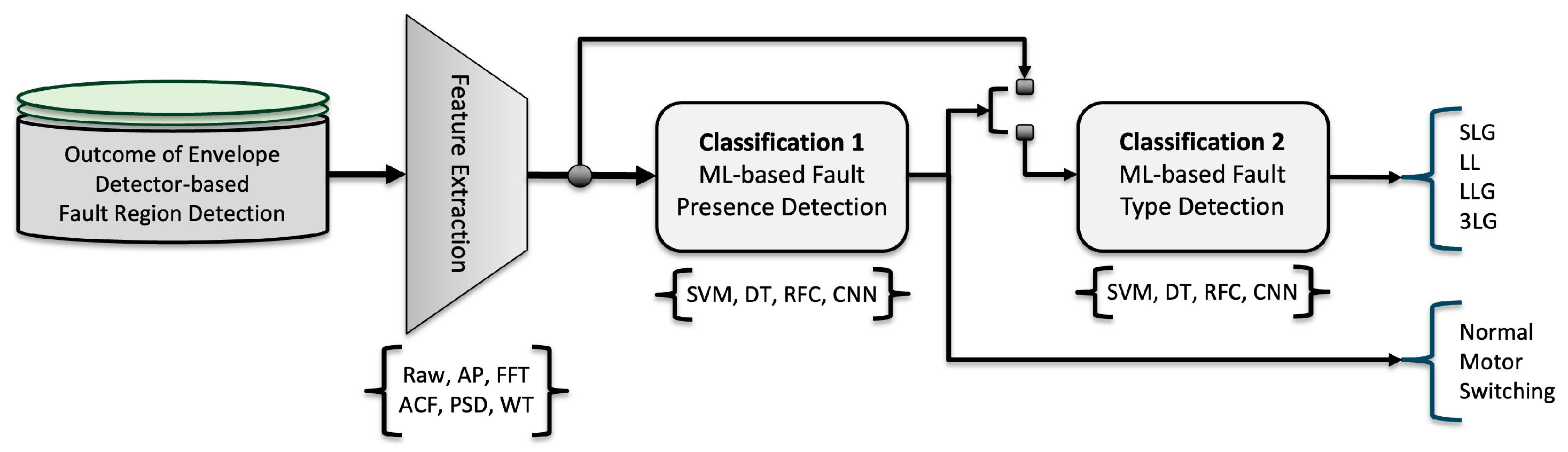
This article proposes a cascaded fault type detection model comprising three main components: anomaly area detection, ML-based fault presence detection, and ML-based fault type detection. The first part uses an envelope-based detector to identify the anomaly region as created in a previous study [37]. However, we enhance this concept by adapting a new filter design to account for the noisier nature of power grid signals collected from meters compared with simulated signals. The second part functions like a switch that determines whether ML-based fault type detection should proceed. It applies the model to detect the presence of a fault in the examined signal by considering four classes (i.e., normal, motor, switching, and fault). If a “fault” is detected in the signal, the second part of the proposed model activates the third part of the system to identify the fault type, including single-line-to-ground (SLG), line-to-line (LL), double line-to-ground (LLG), and three line-to-ground (3LG).
Moreover, in this study, various feature extraction methods (i.e., raw data, AP, ACF, FFT, PSD, and WT) are investigated to achieve maximum prediction accuracy in the ML models of the proposed cascaded system. Additionally, different ML algorithms [SVM, DT, random forest classifier (RFC), and CNN] are evaluated for these ML-based models. To test the proposed method, the electrical distribution grid testbed is emulated in a software environment using different sample rate intelligent electronic devices (IEDs) (i.e., relays and meters) located near and far from the IB-PV array farm. As mentioned earlier, the ML-based fault detection models in the literature are typically trained and tested on datasets created using the same substation configuration or power grid system model. However, these trained models are not well suited for practical cases. Therefore, the dataset for training the proposed system model is generated by a simulation model based on a 46 kV substation, which is not considered in the emulated testbed environment used as a validation set in this study. Consequently, under realistic conditions, the performance of the proposed algorithms is verified using test data prepared with a software–hardware-emulated electrical grid testbed. This testbed uses various sample rate meters, including Schweitzer Engineering Laboratories’ SEL735, SEL421, SEL734, SEL700GT, and SEL351S, positioned near and far from an IB-PV array farm.
2. Distribution System Testbed
2.1. Circuit and Hardware
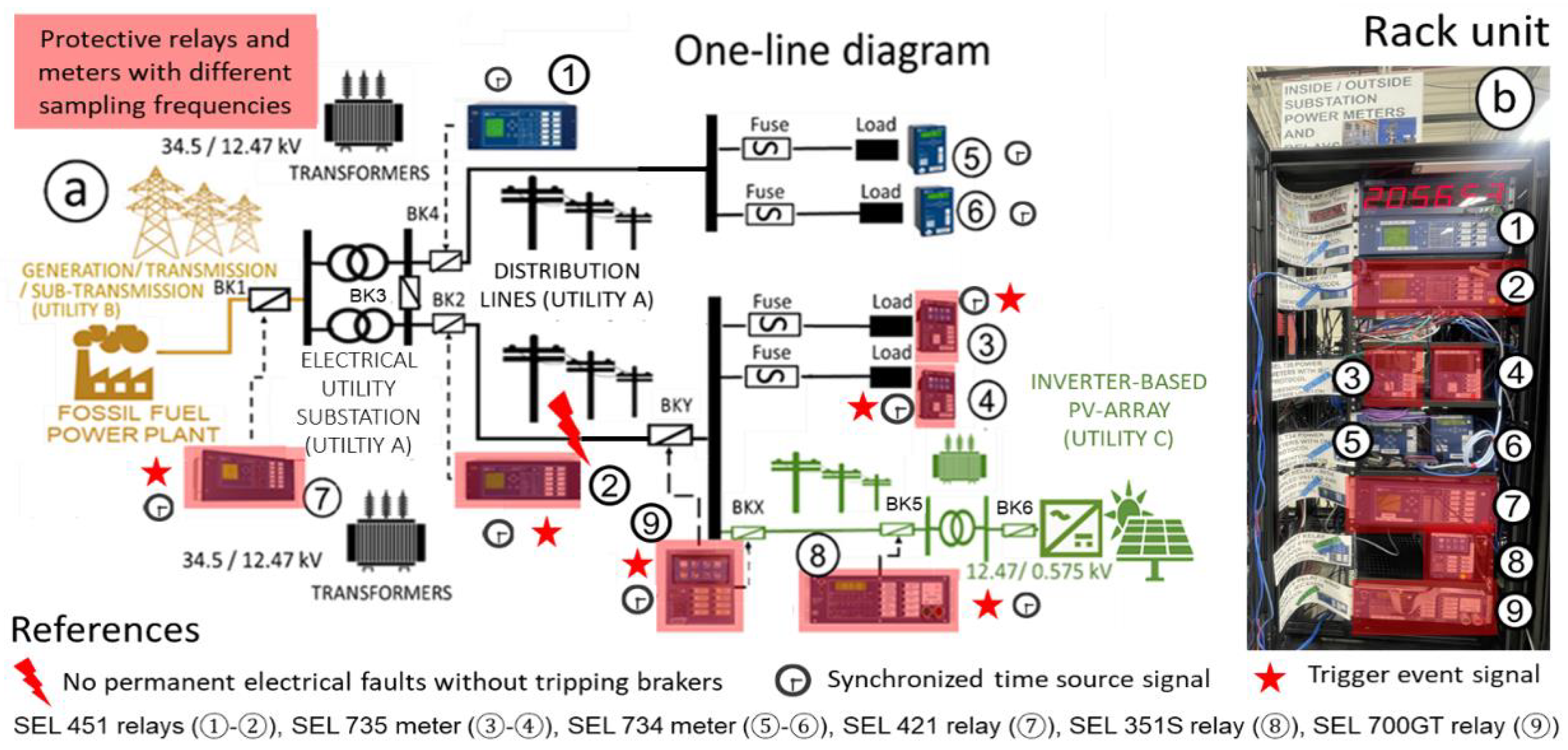
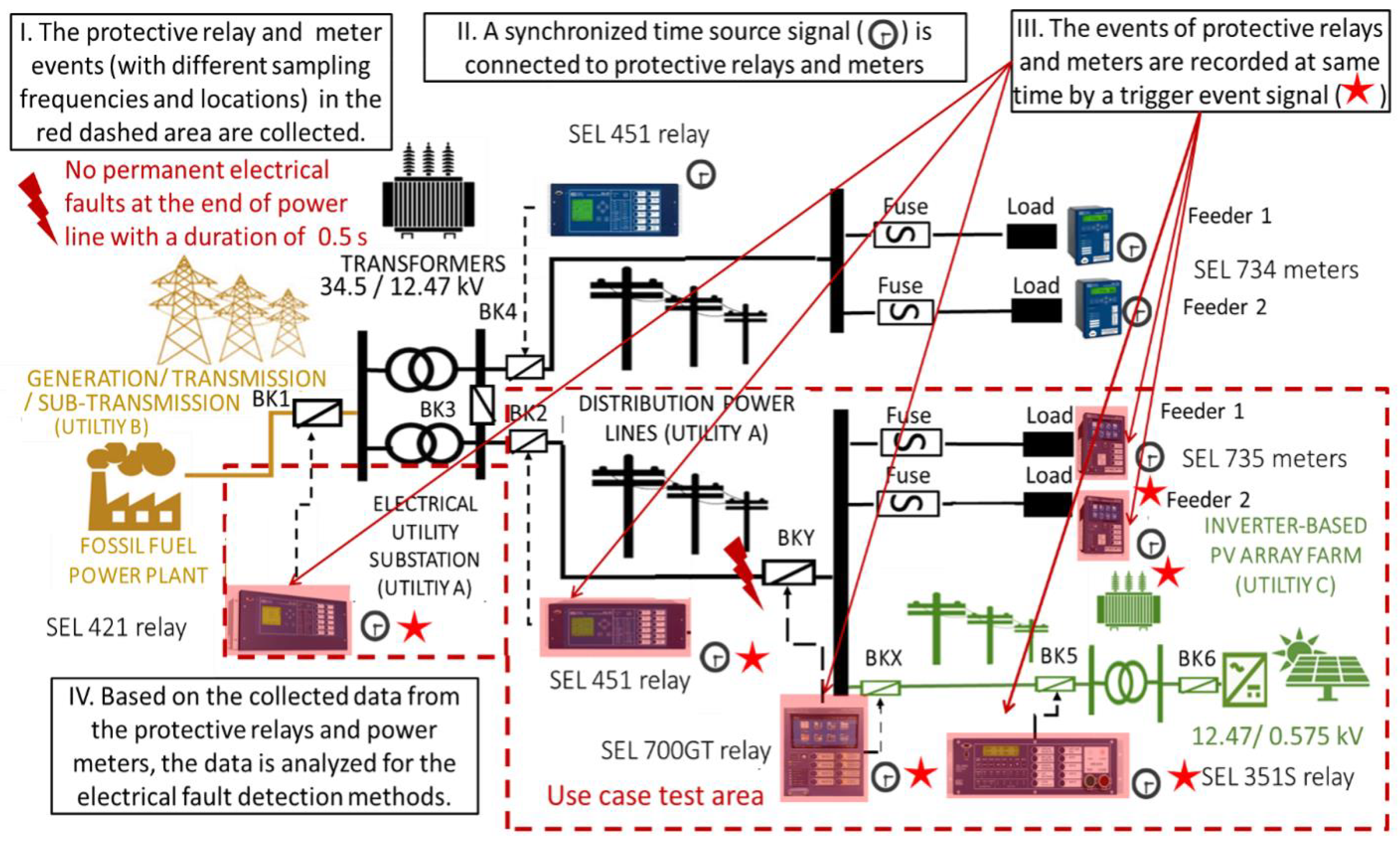
The circuit and hardware of the testbed are shown in Figure 1; the diagram represents an electrical grid/substation with metering devices. This testbed is focused on simulating different electrical fault test use case scenarios. The one-line diagram in Figure 1 represents an electrical substation that has a sectionalized bus system [38] with power transformers and feeders connected to an IB-PV array farm as shown in Figure 1a. The meters and relays in the testbed rack (Figure 1b) are indicated with numerical values, and their locations are shown in the circuit (Figure 1a). The red highlighted relays and meters in Figure 1 are used in this research. This circuit is based on a previous publication in [22]. In Figure 1, the relays and meters are selected based on their protection, measurement or control functions, and locations. The devices numbered 1 and 2 (SEL451) are overcurrent protection relays located at kV side of utility A substation feeders; devices 3 and 4 (SEL735) and 5 and 6 (SEL734) are power meters located on fuse feeders to measure customer loads in utility A; device 7 (SEL421) is a distance protection relay located at kV side of the utility A substation; device 8 (SEL351S) is an overcurrent protection relay located at the kV side of utility C substation; and device 9 (SEL700 GT) is a protective relay with a synchrony check control function located in the point of common coupling between the grid side and IB-PV array side.
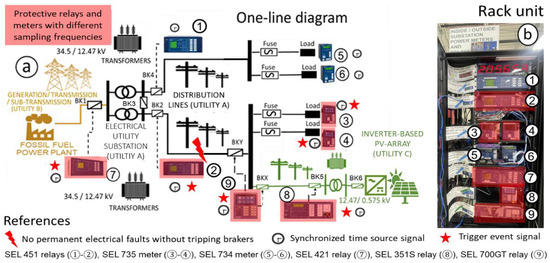
Figure 1.
(a) Diagram of the testbed and (b) real captured photo of equipment rack.
Utility A has a substation with a distribution grid. Utility A’s substation has two transformers with a primary and secondary voltage of and kV, respectively. In this study, the kV power grid with the load feeders is commonly set as a radial system, but it could also be connected to the IB-PV array farm (utility C). Utility C is an IB-PV array farm, and utility B is the fossil fuel source. In the feeder, loads are configured two SEL735 [39] meters and two SEL734 [40] meters. In one power transformer side, a SEL421 [41] relay is set. The SEL451 [11] relays are set at substation feeders. The SEL351S [42] relay is installed at the IB-PV array farm side, and the SEL700GT [43] relay is set at the grid common point of connection. In the real-time simulator (RTS), relays and meters are connected. The relays and meters are synchronized with a time clock system and connected to a trigger recorded event system.
2.2. Substation and Grid Testbed
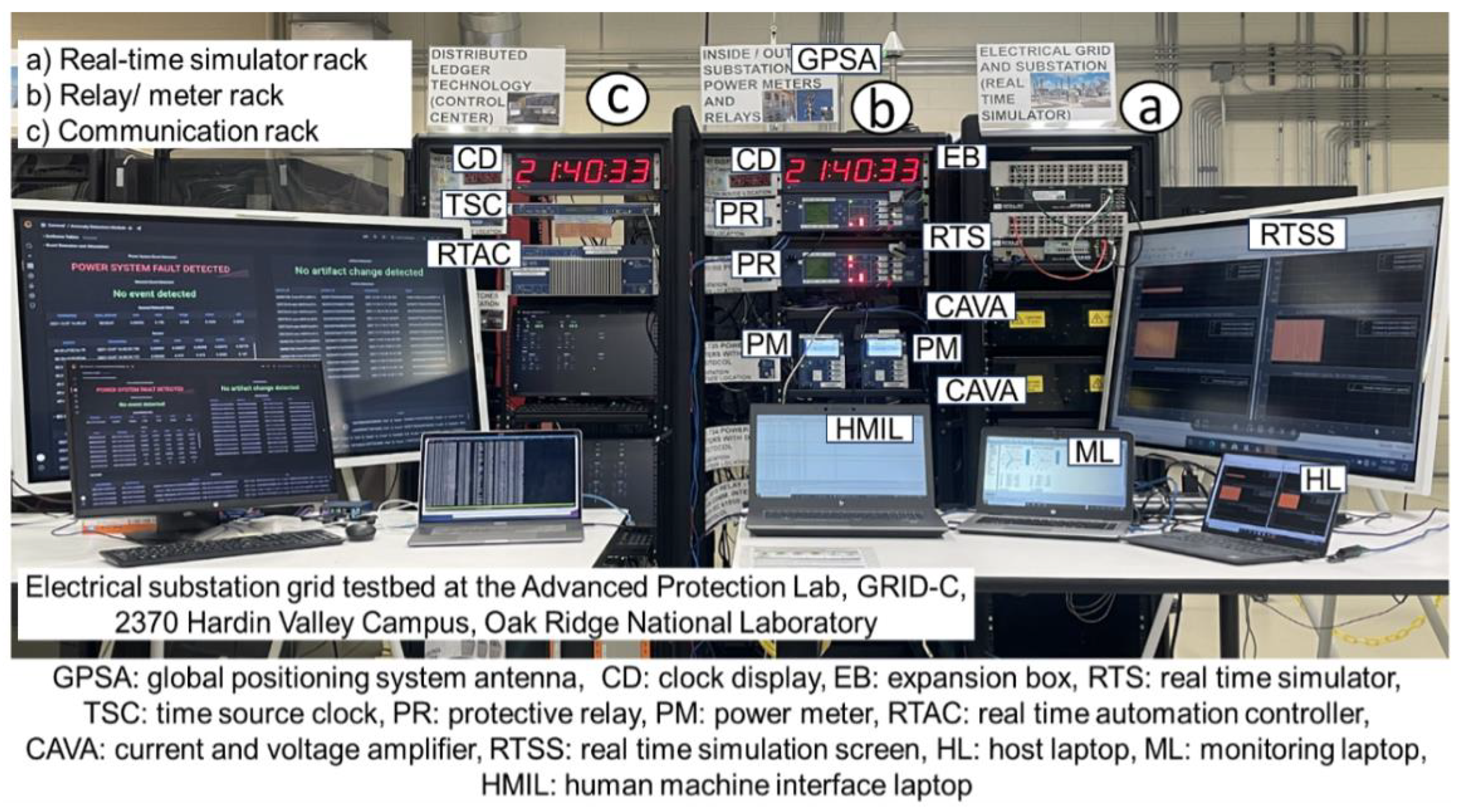
This study uses the testbed demonstrated in Figure 2. The testbed has three rack units. The RTS rack has an RTS expansion box (to increase the number of analog/digital signals) with the current and voltage amplifiers. The relay/meter rack has relays and meters that are wired to the RTS. The synchronized clock with displays are wired to IEDs (relays and meters). The communication rack has a time clock and remote terminal unit. The time clock can generate the time signal with or without a global positioning system (GPS) antenna because it has an internal clock. The advanced electrical substation grid testbed was created and led by Dr. Piesciorovsky [44,45,46]. This advanced testbed has been used in different research areas like harmonics metering [44], distributed ledger technology [45], relays and meters commissioning in electrical grid testbeds [46], and electrical fault type detections. This advanced testbed has been used with different distributed energy resources (DERs). In [44], the testbed was used as a substation/grid with a wind farm to assess the measured total harmonic distortions for meters and relays with different sampling frequencies. In [45], the testbed was used as a substation/grid with a customer-owned wind farm using a cyber grid guard to monitor the power quality using distributed ledger technology. In [46], the testbed was used as a substation/grid without DERs to assess methods for commissioning relays, meters, and real-time simulator testbeds for different power system applications. In this study, the testbed was used as a substation grid with an IB-PV array farm, to assess the envelope- and machine learning-based electrical fault type detection algorithms. Table 1 shows the main research areas, electrical grid characteristics, references, and main deliverables of these studies, using the advanced electrical substation grid testbed.
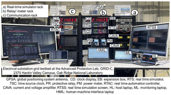
Figure 2.
Testbed established with rack units, including (a) RTS rack, (b) relay/meter rack, and (c) communication rack.

Table 1.
Main research areas, electrical grid characteristics, references and main deliverables of applications using the advanced electrical substation grid testbed.
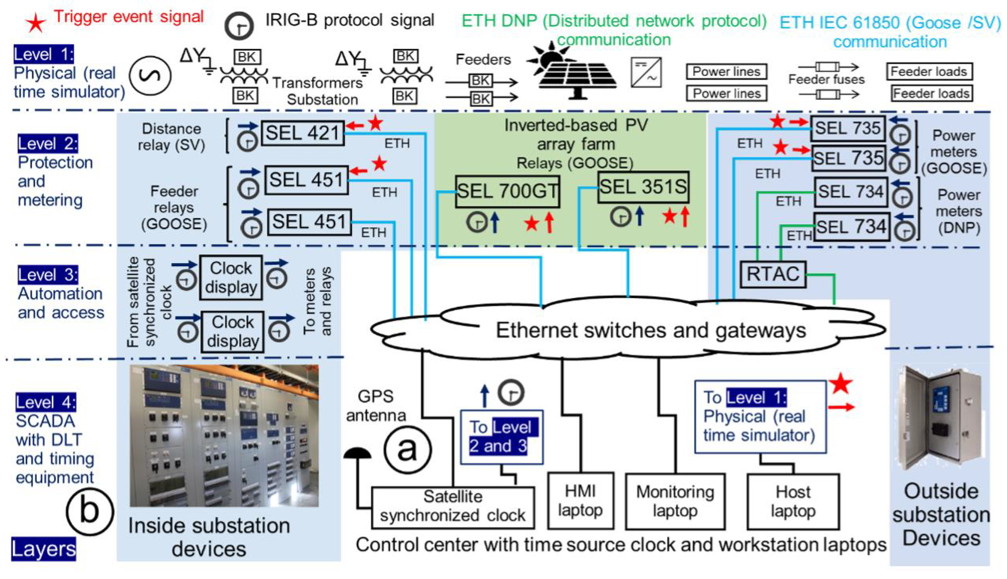
The layers of the testbed are shown in Figure 3. In this testbed, the data are recorded during the simulations. The data are generated by the RTS, and the relays and meters collect these data. The IEDs (i.e., relays and meters) produce the grid data that are synchronized with the time clock system. The testbed’s architecture (Figure 3) have computers and a time clock system (Figure 3a). The physical layers of the electrical substation grid testbed are shown in Figure 3. Level 1 in the physical layers includes the loads, power lines, breakers, transformers, IB-PV array, feeders, and other grid elements. Level 2 is the protection/metering layer that contains the hardware (relays and meters). Level 3 is the automation layer, which includes the clock displays, and communication devices. Level 4 is defined as the control layer.

Figure 3.
(a) Center and (b) levels of the testbed.
2.3. Three-Phase Diagram
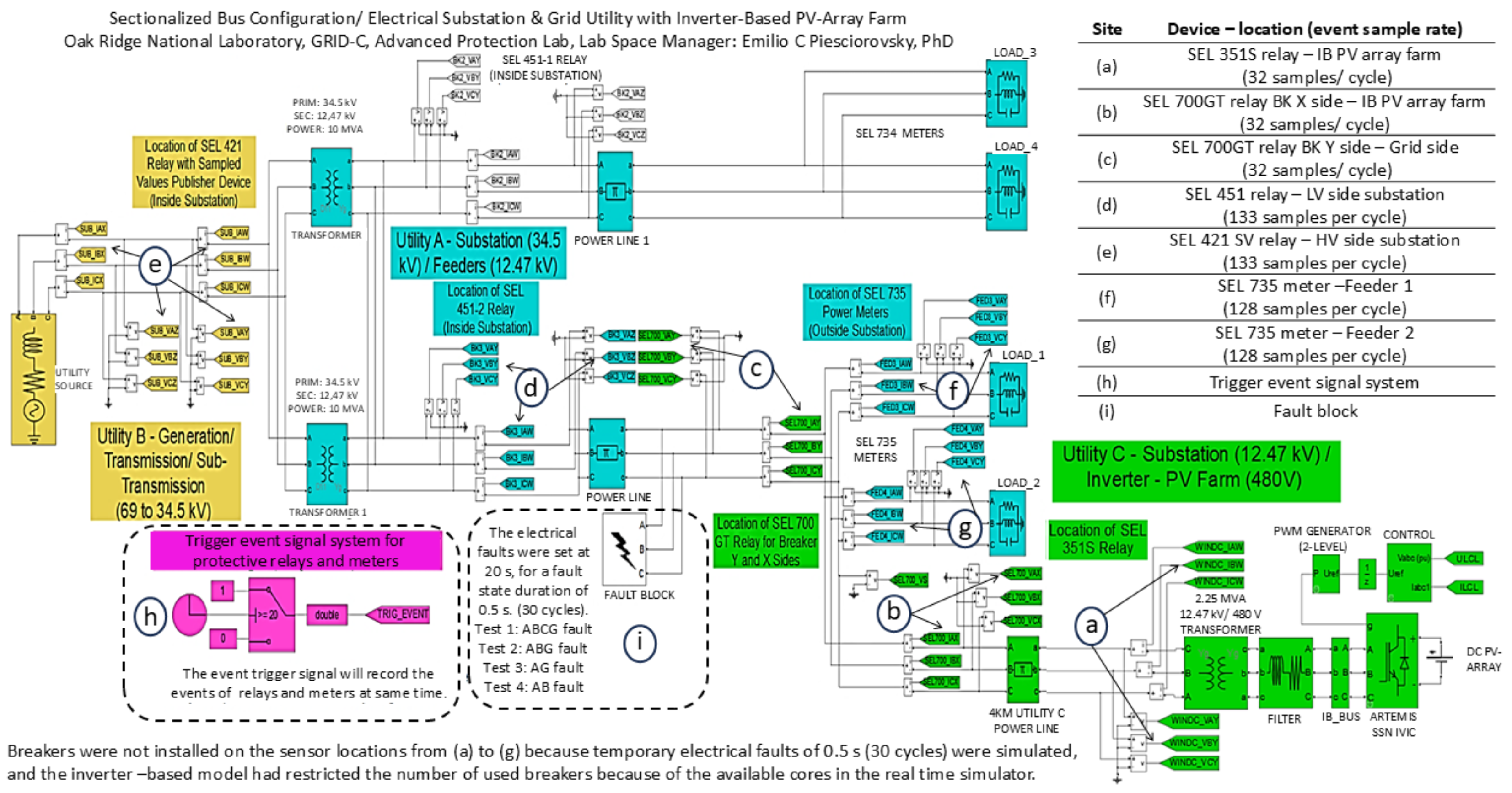
The three-phase diagram of the distribution system testbed was created based on the one-line diagram in Figure 1a. This diagram is shown in Figure 4, and it was created using MATLAB/Simulink (version 2015b). The three-phase diagram has three electrical utilities: the substation grid (utility A) of / kV, the fossil fuel power plant with a transmission/sub-transmission system (utility B) of 69/ kV, and the IB-PV array farm (utility C) of / kV connected to the electrical grid (utility A). Utility A has two / kV transformers connected in parallel and two feeders. Each power line of kV is controlled by a breaker, and the loads are fed by the power lines. These power loads have 50 and 100 T fuses [47]. The three-line diagram is based on a previous diagram used at the electrical substation grid testbed [22,44,45,46], and the IB-PV array farm (utility C) is based on a modified MATLAB/Simulink model to fit there.

Figure 4.
Three-phase substation and grid with IB-PV farm.
In Figure 4, the substation and grid (utility A) are fed by utility B. Utility A consists of the substation, power lines, and loads. Utility C has an IB-PV array farm. The fault resistances for the use case scenarios are implemented into a MATLAB/Simulink three-phase fault block (Figure 4i). It is a programmable phase-to-phase and phase-to-ground fault breaker system that represents the fault ( ) and ground ( ) resistances, snubber resistance (1 × 10⁻⁶ Ω), and infinite snubber capacitance. These values correspond to the default values of the MATLAB/Simulink three-phase fault block. In the electrical faults, the effects of the load current and fault resistance are combined. The fault resistance may be particularly high for ground faults, which represent many of the faults on overhead lines. However, all types of electrical faults are performed in this study. The tests for the electrical faults (3LG, LLG, SLG, and LL) at the power line end of utility A are performed with a fault block, which is presented in Figure 4i. The fault block in Figure 4 is set before running the tests for different electrical fault types and is set to start the electrical fault at 20 s with a fault state duration of s (30 cycles). The relays/meters record their data using the trigger event signal circuit (Figure 4h) that generates the signals for recording the events. In Figure 4, the analog signals at different locations from the IB-PV array and electrical fault site are simulated and collected from meters and relays using no similar sampling frequencies. In the IB-PV array side, the SEL351 (Figure 4a) and SEL700GT relay (Figure 4b,c) record events with 32 samples per cycle. In the electrical substation side, the SEL451 (Figure 4d) and SEL421 (Figure 4e) relays record events with 133 samples per cycle. In the load feeder side, the SEL735 meters (Figure 4f,g) record the events with 128 samples per cycle.
2.4. Time Clock System
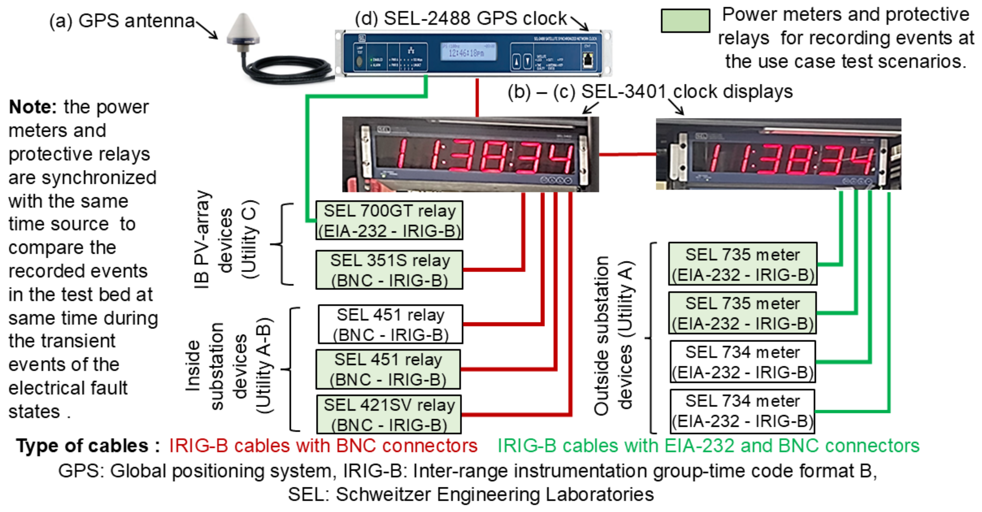
In the testbed, the time clock system is an important tool. It has allowed researchers to synchronize the time of the data collected from relays and meters for the electrical fault and disturbance events. Consequently, the recorded events from the IEDs (meters and relays) could be identified easily after running the use case scenario tests, comparing the time of the IED events at the disturbance initiation. The satellite-synchronized network clock is connected to all IEDs [48]. Figure 5 shows the time clock system with hardware. The primary and backup time frames are defined by the GPS antenna and SEL2488 internal clock [48], respectively. In the testbed, the synchronized time for the metering devices is generated by the internal clock of the time clock system. It performs the time synchronization of all relays/meters with the same time-stamps to identify the recorded events for the electrical fault test use case scenarios.

Figure 5.
Time clock system with metering devices.
2.5. Recorded-Event System
The recorded-event system is a vital tool in the testbed. The signals are generated from the RTS to the IEDs (i.e., meters and relays). In the RT-LAB project, the event signal circuit is built. Figure 6 shows the output card and the signal circuit. As shown in Figure 6a,b, the recorded event system is required to set the time for triggering the signal circuit in the RT-LAB project. In the testbed, the outputs of the event signal circuit are represented by the digital output card of the RTS, which is wired to the relay/meter’s control inputs as presented in Figure 6. The signals of the recorded event system are generated by the clock switch (Figure 6a). The time of the clock switch is set at same time the disturbance event is initiated for the use case tests. The event signals are synchronized at the same time and sent to the SEL relays and meters. As shown in Figure 6, once the event signal is available, the output card from the RTS (Figure 6c) sends a signal to the meters and relays for recording the events at the same time. In the testbed, the event signal circuit is linked to the metering devices’ inputs that receive the DC voltage signal for recording the events.
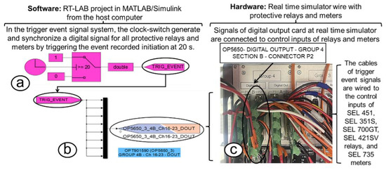
Figure 6.
(a) Event signal circuit; (b) digital output card; (c) RTS.
In the testbed, the relay and meter settings (event total length, sample rate, and pre-length) are defined. Also, the equation of the event trigger signal is defined with a logic condition for recording the events from meters and relays. These logic equations are set as meter and relay control inputs that are wired to the IEDs. The equations of the event signals are set in the metering devices by using a logic “OR”. The IEDs are set using the AcSELerator Quickset software (version ) in the testbed. Table 2 shows the meter and relay settings.
Table 2.
Settings for meters and relays.
3. Envelope Detector-Aided, Machine Learning-Based Fault Type Detection Model
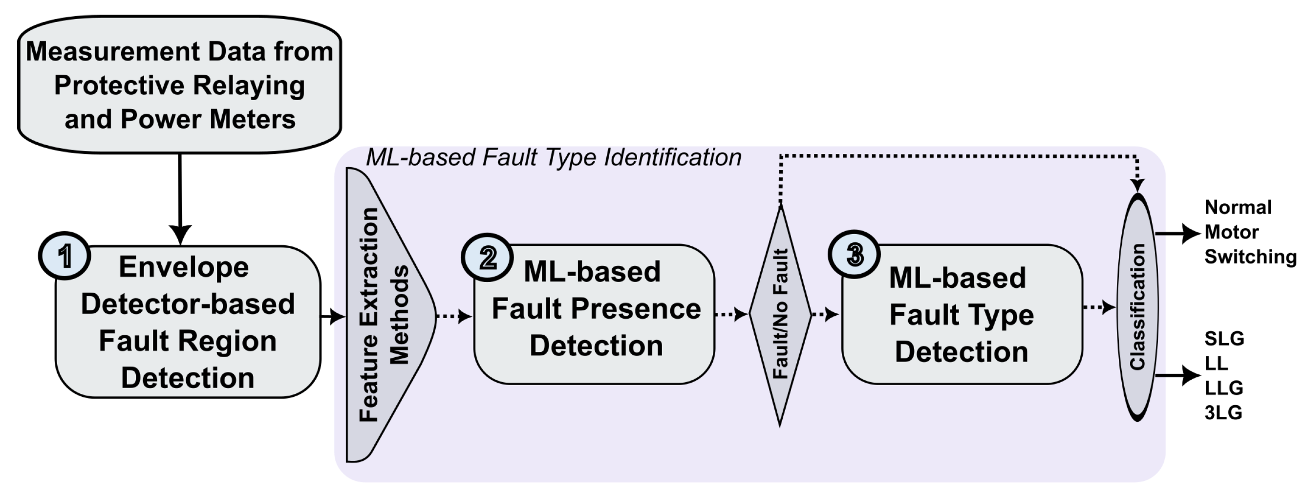
Figure 7 illustrates the proposed fault type detection algorithm. It consists of cascaded structures to identify fault regions, their presence, and types. As shown in Figure 7, measurement data are obtained using relays and meters in the testbed. Initially, the envelope detector-based fault region detection extracts the area of interest from the recorded signals. This process keeps the input sample size constant and removed unnecessary parts for the subsequent algorithms. After applying feature extraction to the clipped signals, the extracted features are input into an ML-based fault detection system. This system categorizes the signals as Normal Condition, Motor, Switch, or Fault. If a fault is detected, the algorithm proceeds to a third step to determine the type of fault. A decision block between the second and third steps determines whether the third step should be run based on the output of the second step. The ML models in both steps are trained for different purposes (the first decides the presence of a fault, whereas the second finds the fault type). This two-step structure was shown in previous studies [35,36] to improve prediction accuracy and decrease prediction time. Finally, in the algorithm’s final step, it identifies the fault types as SLG, LL, LLG, or 3LG.
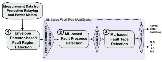
Figure 7.
The block diagram of the proposed envelope detector-aided, ML-based fault type detection model.
3.1. Envelope Detector-Based Fault Region Detection Model
The envelope detector is a well-known method used in various fields to capture changes in the amplitude of a signal. This study extracts the amplitude behaviors of recorded data from relays and meters, which are referred to as the signal’s envelope. We then employ a fault region (start/end times) detection mechanism based on user-defined thresholds. Because the algorithm processes signals without prior knowledge of the input, the algorithm’s precision could be adjusted based on the investigated signal and user preferences. The fault region detection using an envelope detector is established in two steps, analytical signal conversion and fault detection as shown in Figure 8. The first part involves obtaining the analytic signal, and the second part involves extracting the region of the fault area. The algorithm described in [37] has yet to be investigated with noisy recorded signals under different sample rates. Therefore, beyond the study in [37], the algorithm in this work is improved by applying a band-pass filter with a new configuration. This improvement is necessary because the analytical conversion is directly affected by the noise and harmonics caused by a power grid system, meters, or relays.
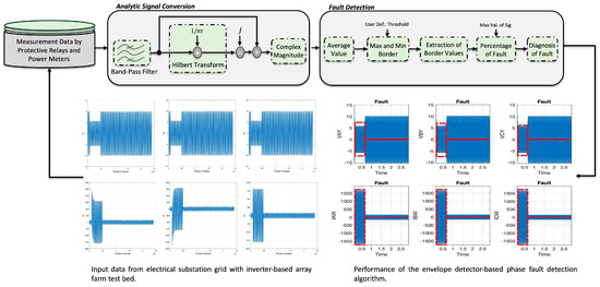
Figure 8.
The block diagram of the envelope detector-based fault region detection algorithm.
As presented in Figure 8, relays and meters apply the band-pass filter to the recorded data. Assuming that the recorded signal is defined as , the band-pass filter’s outcomes can be defined as , where is the band-pass filter operation that removes the noise and harmonics by considering the fundamental frequency of input signal ( Hz). The operation of the analytical signal extraction is named the Hilbert Transform in Figure 8. It fundamentally removes the negative mirror side of the signal and doubles the positive side’s power of the signal in the frequency domain. Thus, the discrete Fourier transform (DFT) operation is employed to filter the signal to obtain its frequency domain as
where N denotes the number of samples of the recorded signal, and K indicates the length of DFT operation that equals the number of samples, , in this study. Then, the analytic part of the signal is evaluated by making the negative mirror frequency side of the signal equal to zero:
where if N is an even number, and if N is an odd number. Therefore, the analytical signal of the recorded signal can be obtained with inverse discrete Fourier transform operation as
As shown in Figure 8, the complex magnitude operation is applied to obtain the envelope behavior of the analytic signal as . Because we do not have prior knowledge of the investigated signal, the fault detection part of the algorithm examines the signal’s envelope to find the fault region’s start/end points. Therefore, the average value of the envelope signal is calculated as , and then the borders are defined based on the user-defined threshold:
where denotes the threshold value that can be defined by the user. In this study, the threshold values are defined based on the relays and meters as defined in Table 3. After achieving the border values of the envelope signal, the border extraction process is applied to the envelope signal as
Table 3.
Threshold configuration for each relay and meter.
Thus, the fault diagnosis operation in the algorithm is employed by considering the maximum changes between the extracted border values and the examined signal, which is defined as . Thus, the phase fault status is defined based on the type of signal, and the percentage of change (Table 3) is defined as
Consequently, the envelope detector-based fault region detection algorithm obtains the region of anomaly based on the diagnosis results, which are given in (7).
3.2. Machine Learning-Based Fault Presence and Type Detection Models
The envelope detector identifies faults’ regions in the examined signal; however, this study uses ML-based models to detect and identify faults. The extracted area of interest in the algorithm’s first part is fed into the ML-based fault presence and type detection model. This section of the algorithm consists of a feature extraction process and two classification layers as shown in Figure 9. Various techniques are investigated in the feature extraction process to obtain the most-effective algorithm. The extracted features are then fed into the first part of classification to recheck the presence of the fault because the envelope detector may not be able to separate the fault from the effects of the motor and switching operations on the examined signal. Therefore, the first part defines the fault presence and provides classification results directly if no fault is detected in the signal. In the case of a fault, the first classification layer triggers the second classification layer to identify the fault type in the signal. In both classification layers, various ML-based models are also evaluated to find the most effective one.

Figure 9.
The block diagram of ML-based fault presence and type detection models.
3.2.1. Feature Extraction Techniques
Because the investigated recorded signal contains various types (i.e., voltage and current) and phases (i.e., A, B, and C), the features of the ML input are established considering all types. Thus, is one of the recorded signals so that define the type and phase of the signal as given in Table 4.
Table 4.
Defined numbers of various signal types and phases used in the feature extraction process.
Notably, the feature extraction methods are expressed by considering that the CNN architecture is used in the ML blocks in the algorithm. For this reason, the feature extraction methods’ outcomes are designed as matrix forms; however, they can easily be converted to vector forms using vector conversion algorithms and applied to other ML algorithms (SVM, DT, and RFC).
Raw Data
In this technique, the input data of the ML model are prepared without any signal processing techniques to observe the achievement or drawbacks of any signal processing techniques. Therefore, the input matrix for the ML block is ready for raw data by combining whole types and phase-in together as
Fast Fourier Transform
The FFT process is employed to observe the frequency behavior of fundamental signals and harmonics with noise. These signals and harmonics are used as inputs for ML models to find changes based on fault. Thus, the DFT operation is employed to obtain the frequency domain components of the analyzed signal, which is also used in (1) as [49]:
Before the creation of the feature matrix model for FFT, half of is removed as , where because the includes the same positive and negative sides of the frequency domains. Then, the feature matrix model is created for FFT as
Amplitude and Phase
The effect of fault can easily be observed in the amplitude and phase values of a signal that behaves differently than usual. Thus, the amplitude and phase information of the signal is used to establish the matrix model as
where shows the amplitude of signal, and .
Autocorrelation Function
The ACF obtains repeated patterns in a noisy environment. As a result, the ACF can be used for feature extraction methods. Thus, the ACF of the examined signal can be calculated as [50]:
Thus, the feature matrix for ACF can be created using both halves of the calculated components as
Power Spectral Density
The signal strength is another feature set that can be obtained with the power of the signal. Thus, by using (9), the feature matrix for PSD can be created [35]:
Wavelet Transform
The WT is a common method to investigate power signals at different band filter levels and can provide changing sampling information with a Shannon Entropy calculation at each decomposition level [51]. Thus, the Shannon Entropy of each decomposition level for the recorded power grid signal is obtained to observe information changes as
where is the number of samples at the rth decomposition level, and R indicates the number of the decomposition value. In (15), shows the probability of energy at the rth decomposition level that can be defined as
where is the high-pass filter outcome in the filter-bank algorithm designed for WT calculation that is defined as [52]:
where is the filter that is designed based on the Daubechies wavelet signal. Notably, the bank filter is established as a cascaded design with high- and low-pass filters. In (17), the first input signal is the investigated signal , but the input signal changes with the low-pass filter’s outcomes when the decomposition number is increased. For instance, the input of (17) is for , and other decomposition values (i.e., ) are defined with a low-pass filter, which is defined as
where g is the low-pass filter signal. Therefore, the feature matrix for WT can be established using (15):
3.2.2. Machine Learning-Based Classification Layers
Both classification layers in Figure 9 are tested with various ML algorithms. The considered ML algorithms are well-known techniques, including CNN, SVM, DT, and RFC. Each ML algorithm is trained with the created dataset. For the training dataset of the ML models, a simulation model is designed in a MATLAB Simulink environment by taking into account the parameters of the 46 kV substation, which is different from the Figure 2. Basically, we train our model with another substation and apply the trained model to detect the faults in the testbed utilized in this study. The substation model used in the training model has feeders with transformers, capacitor banks, line impedances, and individual loads. As the purpose of ML models is either finding the presence of fault or classifying the type of fault, various fault types are used at the end of each feeder. As we need more different datasets for each specific type of fault, we change the main components of each training datum such as the analog-to-digital converter noise, the load percentage of network, bit number, and start/end sample points of faults. The training process for each ML algorithm used 2113 sample data created using parameters of the real 46 kV substation. However, the training dataset is divided into for training and for validation because the validation data are used to monitor overfitting during the training process. If there is an increasing gap between validation and training performance, the training operation is automatically stopped to avoid overfitting. Because both classification layers are used for different purposes, the training labels and datasets can be different even though they have the same architectural design. The first classification layer is designed to identify a fault in the power signal and separate the fault signal from the switching and motor signal waveforms commonly available in power grids. Therefore, the labels for the first classification layer’s dataset are prepared considering the Normal Condition, Motor, Switching, and Fault. The second classification layer aims to identify the common types of faults, so the labels for this layer are designed as SLG, LL, LLG, and 3LG. Because of the changes in the size of the feature extraction outcomes and label number, the structure of the ML architecture is adjusted, and models are created for each possible variation to achieve the maximum performance in this study.
Convolution Neural Network
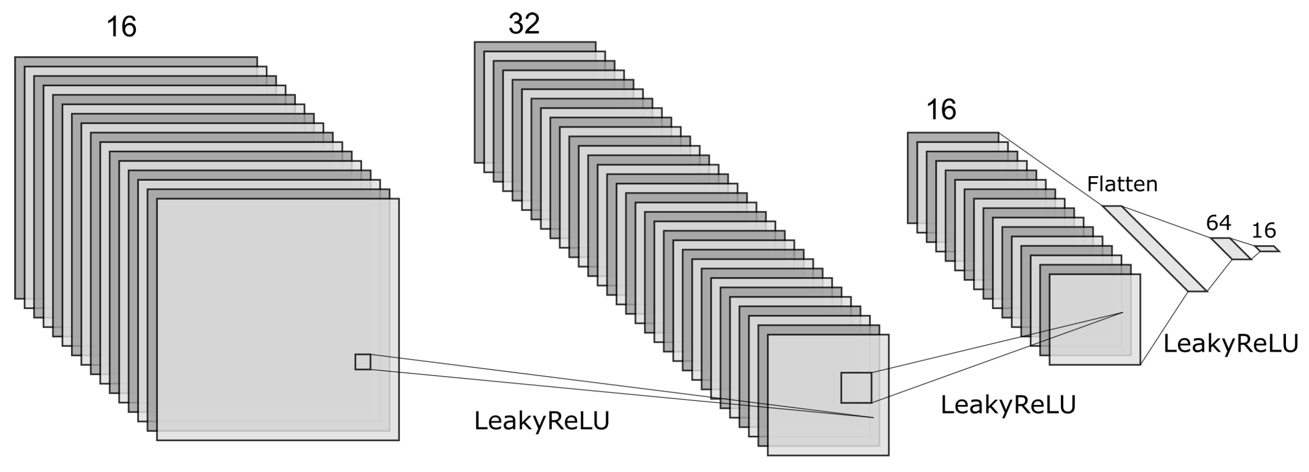
The empirically designed CNN architecture for both classification layers is presented in Figure 10. Because the input size can change based on the feature extraction methods, the channel length numbers are only given in Figure 10. The CNN is established with three convolution layers, and the channel lengths of these layers are 16, 32, and 16, respectively. After each convolutional layer, the Leaky ReLU is employed to prevent vanishing problems in the ML layers. As illustrated in Figure 10, the last convolution layer is shaped as flattened layers, and then the flattened layer is connected to two fully connected layers. The lengths of the fully connected layers are empirically adjusted as 64 and 16. The last layer is the softmax layer configured as 4 for both classification layers because the number of labels for each classification layer is the same.

Figure 10.
The illustration of designed convolution neural network (CNN) model.
Support Vector Machine
SVM is another ML technique that aims to maximize the space between the defined hyperplane and the nearest data points [31,35]. When dealing with datasets containing more than two labels, optimizing the SVM model can be challenging. For this reason, a polynomial order of four is used to achieve the highest prediction accuracy in this study. Additionally, a one vs. one decision function is employed for the multilabel design.
Decision Tree and Random Forest Classifier
The DT algorithm analyzes the training dataset and labels using a tree-like structure consisting of various nodes (root, decision, and leaf). This structure determines the label for the test data by splitting the dataset into subsets based on the most significant feature. The RFC is an improved version of DT constructed from the collection of DT structures.
4. Testbed Model and Use Case
4.1. Testbed Model
The emulated software–hardware electrical grid testbed is set up with an OP5600 real-time simulator (Opal-RT Corporate, Montréal, QC, Canada)/expansion box with relays/meters in the loop. The real-time simulator is connected to a host computer that is used as an interface to set the test scenarios based on running different temporary electrical faults and selecting the duration of the simulations around 50 s. The emulated software–hardware electrical grid reflects a real-world grid condition because it uses relays and meters in the loop and the simulations are performed with a time step of 50 μs to solve electrical system models and reproduce the nature of electrical events. The testbed model is shown in Figure 11. It is formed by the substation grid that is connected to the IB-PV farm. The meters and relays that are in the red dashed area have different sample rates. In the testbed model, data from the relays and meters are recorded at same time. Therefore, the recorded events from the meters and relays are collected at the same time by using the event signal system.
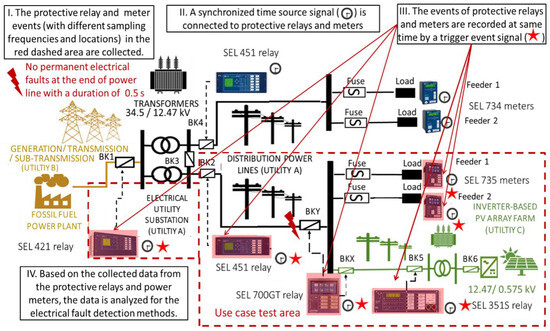
Figure 11.
Circuit for the testbed model.
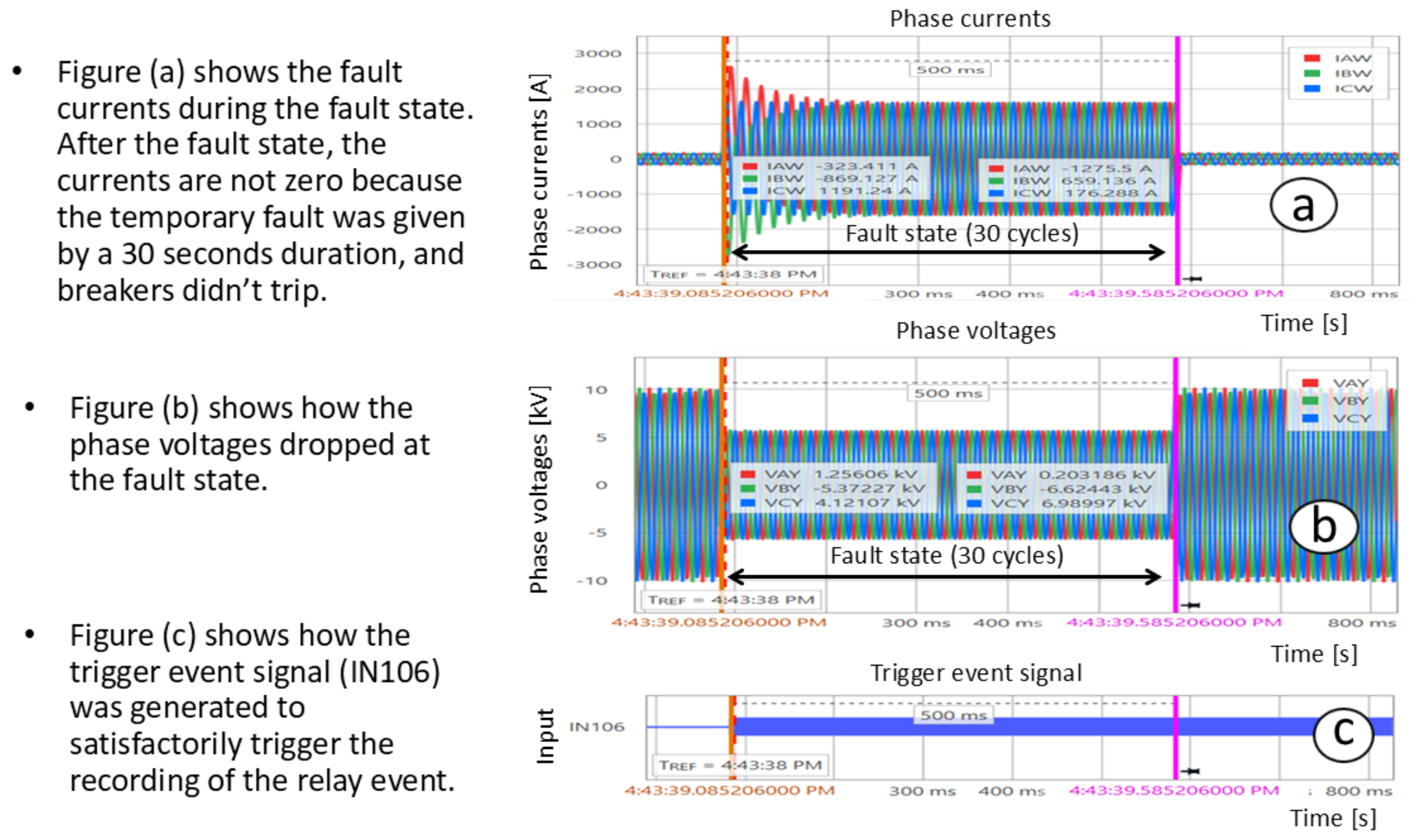
From the saved relay and meter events, the data (i.e., phase current and voltage signals) are analyzed, and the envelope- and ML-based electrical fault type detection algorithms for the electrical distribution grid with different sample rate relays/meters located at different sites from the IB-PV-array farm are assessed in detail. The test scenarios are based on assessing these algorithms for different temporary fault types at the distribution line of utility A as shown in Figure 11. These temporary electrical faults have a duration of s (30 cycles), and the testbed is prepared for the relays that do not trip the breakers for recording and saving the whole fault states in all protective relays and meters.
4.2. Test Scenarios
The test scenarios for the IB-PV array farm are based on simulating different electrical faults. Four electrical fault tests are performed, and data are collected from six IEDs at the same time. In the IB-PV array farm with the electrical grid, the 3LG, LLG, SLG, and LL electrical faults are simulated. Each fault simulation test is run for approximately 50 s, and the loads are fed by utilities A and C, which are a grid source and IB-PV-array farm, respectively. Then, at 20 s, the temporary electrical fault with a duration of s (30 cycles) is performed at the power line end of utility A. The relays do not trip breakers because the testbed is set for recording and saving the whole fault states in all relays and meters. In these tests, the recorded events from four relays (SEL351S, SEL700GT, SEL451, and SEL421SV) and two meters (SEL735) are collected. Table 5 shows the characteristics of relays and meters for the electrical fault test use case scenarios.
Table 5.
Characteristics of IEDs for electrical fault test scenarios.
The relay and meter events are obtained using the AcSELerator Quickset software (version ) The voltages, currents, and event trigger signals are plotted by the SynchroWAVe software (version ) [53]. The relay and meter events have different sampling frequencies and, consequently, different sample rates. The events from the relays and meters are collected as COMTRADE files and converted into MATLAB files to run the assessment of the proposed envelope- and ML-based electrical fault type detection algorithms.
5. Results
5.1. Relay and Meter Events
The substation grid testbed with the synchronized time system and event signal system for the relays and meters is evaluated satisfactorily by performing the electrical fault test scenarios without tripping breakers with an IB-PV array farm model. The tests are based on a simulation of approximately 50 s (Figure 4). Then, temporary SLG, LL, LLG, and 3LG electrical faults of 30 cycles at the power line end are set at 20 s. Table 6 shows the identification events collected from the relays and meters. Figure 12 shows the data from the SEL451 relay for the temporary 3LG electrical fault.
Table 6.
Events collected for the electrical fault tests.
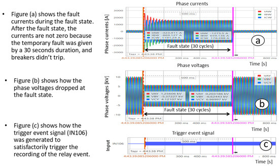
Figure 12.
The SEL-451 recording signal samples, including (a) currents, (b) voltages, and (c) digital signal plots for 3LG fault test.
In the use case tests, the recorded event system is triggered at 20 s, and the signal is received by all relays and meters at same time. This result allows the recorded events to be synchronized for all IEDs (meters and relays). These events are collected using the AcSELerator Quickset software (version ). All devices are stamped with the same time for each event test, allowing us to identify and select the relay/meter events for each use case test. The plots for the currents, voltages, and event trigger signal are made by using the SynchroWAVe software (version ) [53], as shown in Figure 12 for the SEL451 relay.
5.2. Envelope-Based Fault Region Detection
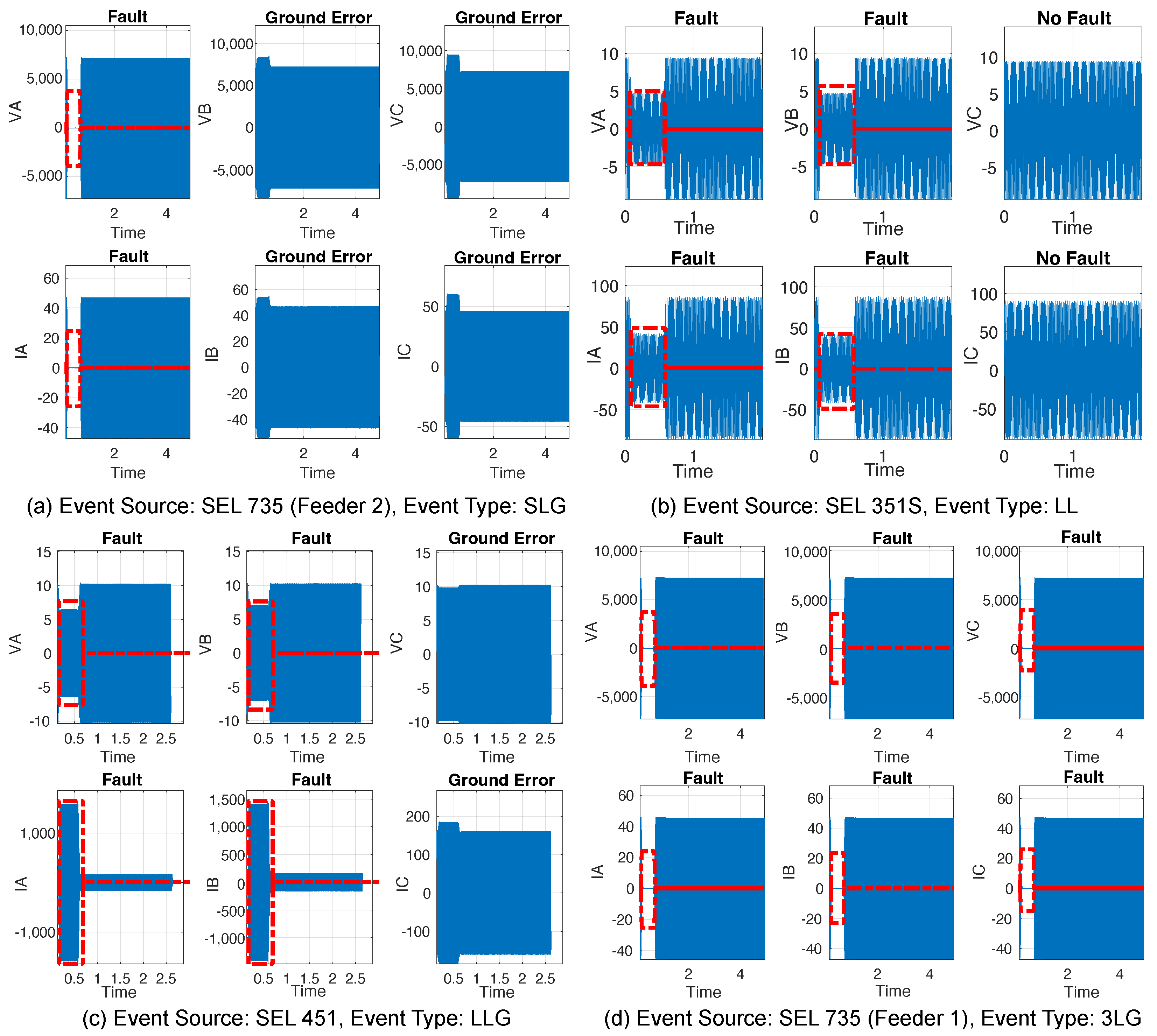
Figure 13 shows the performance of the created envelope-based fault region detection algorithm with recorded events from different relays and meters. In the test, we consider various event types (i.e., SLG, LL, LLG, and 3LG) to indicate the proposed method precision. As shown in Figure 13, each type and phase type of the signal are assessed to locate the start/end points of the fault region. Also, the algorithm defines the event based on the user’s defined threshold values. Subsequently, Figure 13a shows an example of the SLG type of signal recorded by the SEL735 (Feeder 2) meter. The result indicates that the proposed method can identify which phase has a fault and its start/end points. As shown in Figure 13b, the test is also applied for the LL type using the SEL351S recorded data. The algorithm still maintains its prediction performance. The algorithm’s performance is also verified for LLG and 3LG fault types, analyzing the recorder signals by SEL451 and SEL735 (Feeder 2), respectively.

Figure 13.
Results of the envelope-based fault region detection algorithm with various fault types and relays/meters (fault regions are indicated with red lines, as estimated by the designed method).
5.3. Machine Learning-Based Fault Presence and Type Detection Models
The performance result of the ML-based fault presence detection algorithm is indicated by testing with 20 recorded data from the testbed as given in Figure 14. The various ML-based models and feature extraction methods are used in the test process to find the best option for fault detection. It should be re-emphasized that the training model is trained with the 46 kV substation simulation environment’s dataset, created based on another substation, and has never been used in the testbed. However, the results are shown using a test dataset from the designed testbed.
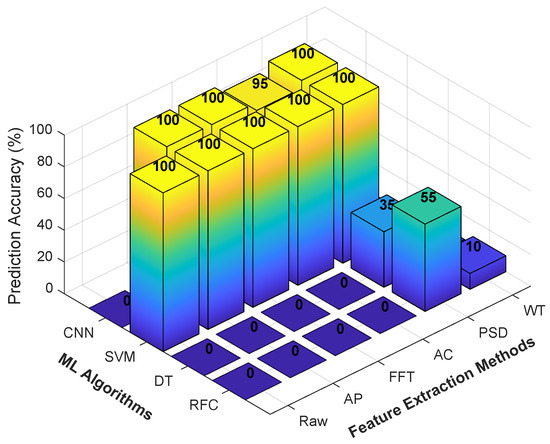
Figure 14.
The prediction accuracy of ML-based fault presence detection (classification layer 1) algorithm with different ML methods and feature extraction techniques.
Further, each combination of ML algorithms and feature extraction techniques is tested with all recorded data from all meters or relays. To clarify, a single model is employed for the entire test dataset; however, we increase the variation of the single model by applying different ML algorithms and feature extraction techniques to identify the best ML-based fault presence and type detection model.
As shown in Figure 14, the prediction accuracy of ML-based fault presence detection is presented in two perspectives: one is ML algorithms, and the other is feature extraction methods. In terms of ML algorithms’ performance, CNN and SVM models provide the maximum prediction accuracy results compared to DT and RFC. Due to the constant tree structure that is not flexible, the prediction accuracy rates of DT and RFC are low for this application. Another reason for this performance decrease on DT and RFC is that the training dataset created using the simulated data of 46 kV substation was never used in the testbed.
In the training process of SVM, the polynomial equation was evaluated to find optimal border between four labels (normal, motor, switching, and fault). The SVM method indicates the best performance prediction accuracy in whole feature extraction methods because each label has unique specific behavior that easy to separate by SVM. The CNN processes patterns and is typically used with image data (2-dimensional data). If the features cannot provide some obvious pattern, the performance of CNN is decreased. As given in Figure 14, the performance of CNN with raw data is because the pattern on the data may break down due to the 2-dimensional conversion of raw data (the vector raw data are split and combined to obtain matrix data suitable for the CNN input). However, the CNN provides promising accuracy with the combination of the amplitude and phase features (AP), frequency domain (FFT), hidden patterns (ACF), and the combination of the time and frequency domains (PSD). The WT is well-known method to find any frequency change in the time domain, which helps to figure out the start/end points of a fault; however, it cannot provide distinct features for fault presence detection application as seen in Figure 14. Accordingly, each ML method cannot achieve significant performance from the WT-based feature extraction technique. Consequently, the CNN and SVM algorithms with the AP, FFT, ACF and PSD techniques provide the best performance for fault presence detection application.
In Table 7, the classification layer 1 in the proposed model is analyzed with different performance metrics: precision, recall, and F1-Score. Herein, the precision shows how often ML models do correct prediction; recall indicates the frequency of correct label identification; the F1-Score shows the overall performance by considering both the precision and recall performance metrics. Also, each performance metric is indicated between 1 and 0, where 1 is the best and 0 is the worst. As presented in Table 7, each feature extraction technique is investigated with various ML algorithms. The results reveal that DT and RFC algorithms are worst at each feature extraction technique. For instance, each performance metric of DT and RFC is 0 with raw data, AP, FFT, ACF, and WT. On the other hand, the CNN and SVM perform best by employing AP, FFT, ACF, and PSD feature extraction techniques. Except WT and Raw Data, each feature extraction technique provides valuable features for CNN and SVM algorithms to classify labels of data with high precision and recall, but their prediction time varies due to the computational complexity of feature extraction techniques.
Table 7.
Different performance metric results of ML-based fault presence detection (classification layer 1) algorithm with various feature extraction methods with ML algorithms.
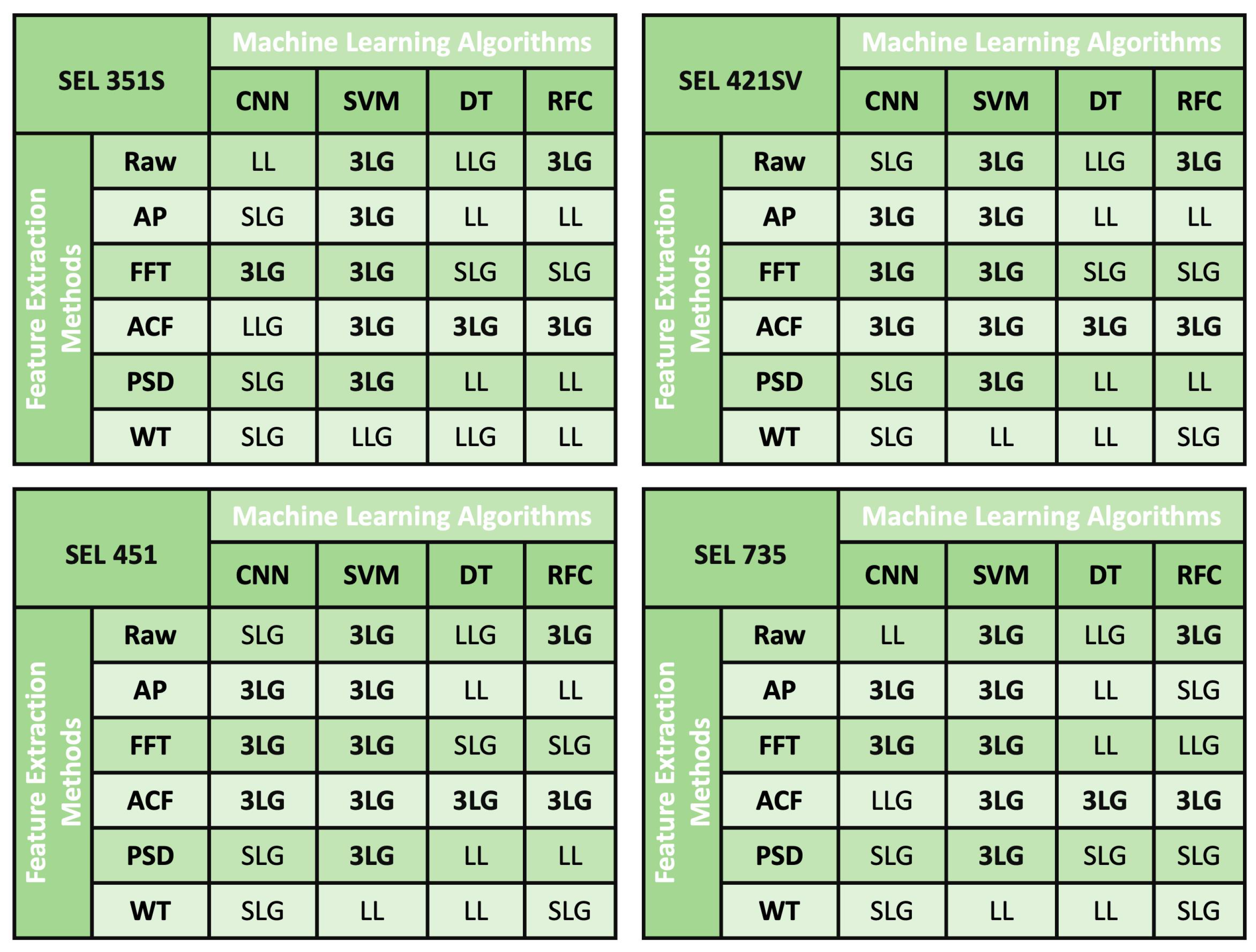
The ML-based fault type detection performance measurement is performed by using different relays and meters’ recording data as shown in Figure 15. The predicted outcomes are given in Figure 15 to investigate the response of each ML algorithm and feature extraction method. The 3LG fault type is considered for the test, and the results are indicated with various power relays and meters to investigate the impact of the sample rate and electric grid location of measurement devices. Outcomes reveal that the prediction accuracy is slightly affected by the sample rate measurement devices. For instance, the CNN performance is decreased with the SEL351S, which has 32 sample rates. However, as obtained in the previous results in Figure 14, the SVM shows significant results by making accurate predictions with each feature extraction method except WT. Further, the FFT feature extraction method provides true prediction with the CNN method. The CNN and AP combination can also achieve reasonable results, but other feature extraction methods (i.e., raw data, ACF, PSD, and WT) cannot provide accurate predictions. In the case of other conventional ML algorithms, both DT and RFC only make one correct estimation. In general, the SVM and CNN algorithms perform well in the ML algorithms, and ACF and FFT provide more accurate results than the others.
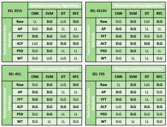
Figure 15.
The prediction accuracy of ML-based fault type detection (classification layer 2) algorithm with different ML methods and feature extraction techniques for 3LG fault with respect to SEL351S, SEL421SV, SEL451, and SEL735.
The ML-based fault type detection (classification layer 2) is also verified with different performance metrics as presented in Table 8. In this case, all 3LG fault types from testbed are used to measure precision, recall, and F1-Score. Each feature extraction and ML technique is employed. As for pure data (raw data), SVM and RFC provide significant performance; however, the same success of the RFC algorithm cannot be achieved with other feature extraction techniques. Results in Table 8 clearly show that the highest precision and recall can be obtained with the CNN and SVM algorithms along with the AP, FFT, ACF, and PSD techniques. Since ML algorithms are trained on simulated data, their performance is limited by the similar characteristics of labels extracted by using feature extraction techniques. For these reasons, it is necessary to examine not only the prediction accuracy but also the processing times of classification layers 1 and 2.
Table 8.
Different performance metric results of ML-based fault type detection (classification layer 2) algorithm with various feature extraction techniques with ML algorithms. This measurement considers 3LG fault with respect to all power relays and meters.
The processing time of the ML-based fault type identification is presented in Figure 16. The processing time of one datum is measured by considering the specific feature extraction method and ML algorithm. The proposed method is run on the 2023 MacBook Pro (Apple Inc., Cupertino, CA, USA), which has an Apple M2 Max chip, 12-core CPU, 30-core GPU, and 16-core Neural Engine. In Figure 16, the ACF method is excluded due to its extremely high processing time (around s), which ruins the graph visually. Although, the DT cannot provide sufficient prediction accuracy, the lowest processing time is obtained using the DT with FFT method. SVM is the best in the prediction accuracy; however, the computational complexity of SVM fails, with the highest processing time with each feature extraction method. The results reveal that CNN with FFT provides the optimal solution for high prediction accuracy and low processing time in the ML-based fault type identification task of proposed scheme.
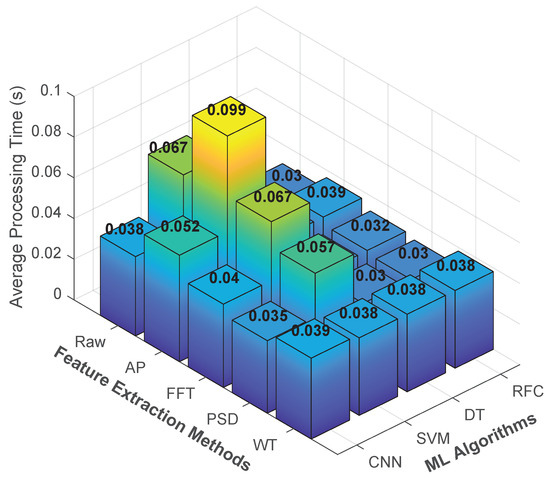
Figure 16.
Total processing time of ML-based classification layers by considering different ML methods and feature extraction techniques.
6. Discussion
Under real-world conditions, this study tested the fault region presence and type detection algorithms for the emulated electrical substation with an IB-PV array farm. The foremost significant contribution of this study, beyond other studies in the literature, was employing the ML algorithm, which was trained based on the simulation data created with a completely distinct substation model. In the literature, many studies on ML-based fault detection algorithms were tested considering the same substation parameters used for training operations. Please note that data generation is a lengthy process, and it is not always possible to obtain enough data to train a model. However, it was shown in this study that we used a training model from another substation and applied to the distribution system testbed explained in Section 2.
The designed model from the 46 kV substation simulation environment consisted of three main processes: finding the fault region in the data, checking the presence of the fault, and defining the type of fault. The first part of the model was created using an envelope detector-based fault region detection algorithm that was improved from the previous study to achieve higher precision. This part was investigated using data collected from various relays and meters. Because the relays and power-meter hardware components may vary, test data were recorded at different sample rates. However, these variations were effectively avoided in the algorithm’s performance by adjusting threshold values based on the relays and meters in the envelope detector-based fault region detection algorithm.
The second part of the model separated the fault signal from the effect of switching and the motor in the power grid systems. This part was examined using various feature extraction methods and ML algorithms. Because the DT and RFC had tree structures trained based on the other substation, their prediction accuracy was with various feature extraction methods except PSD and WT. However, the estimation performance was achieved with SVM and CNN ML algorithms, but the raw data structure could not provide valuable features for CNN algorithms. For this reason, the ML-based structure in the proposed model was verified with various ML algorithms and feature extraction methods. The third part of the model found specific fault types of the test data. This part was also analyzed using different ML and feature extraction methods. The results revealed that the prediction accuracy for fault type detection was decreasing because the ML models were trained considering different substation parameters. The final results suggest that the specific fault type detection model should be improved to perform better under real-world conditions.
7. Conclusions
This study assessed envelope-aided ML-based electrical fault type detection algorithms for electrical distribution grids with an IB-PV array. The electrical substation grid emulation was established by considering three utilities (utilities A, B, and C). Utility A included a substation ( kV) and feeders ( kV) fed by utility B. Subsequently, utility B consisted of the generation, transmission, and sub-transmission of a grid. Furthermore, utility C was designed with a substation ( kV) and IB-PV array farm. The power grid signals were recorded in the emulated substation using relays and meter equipment. The examination of the proposed algorithms was executed using these recorded power grid signals. The main achievement of this examination was that the ML-based models were trained by considering another substation configuration but were tested with modern electrical grids’ measured power signals. The results provide valuable insights for smart grid systems that leverage the protection and control of power grid systems. For instance, under the test of data from various power relays and meters, the envelope-based fault region detection algorithm obtained an area of interest in the signal (start/end points of fault) precisely. Further, the first ML-based fault presence detection model achieved prediction accuracy and F1-Score by using the SVM algorithm with raw data, the AP, FFT, and PSD features, and the CNN algorithm with AP, FFT, PSD, whereas the second ML-based fault type detection model on specific fault type also reached prediction accuracy and F1-Score with the same ML algorithms and feature extraction method combination. However, the processing time of the algorithms demonstrated the optimal combination for ML models, which was achieved with the SVM algorithm with the PSD feature ( s average processing time) and the CNN algorithm with the FFT feature ( s average processing time).
Further, as outlined in the IEEE 242 standard [54], the fundamental features of power grid protection system applications specify that the maximum response times for primary and secondary (backup) protection equipment are defined based on the specifications of the relevant power system and fault conditions. In future research, we plan to investigate the applicability of the proposed method in a real-world scenario, taking into account end-to-end time measurements, including fault identification, signal propagation, and protection activation.
Author Contributions
Conceptualization, O.A., E.C.P., A.R.E., N.S.; methodology, O.A., E.C.P., A.R.E., N.S.; validation, A.R.E.; formal analysis, O.A., E.C.P., A.R.E.; investigation, O.A., E.C.P., A.R.E.; resources, O.A., E.C.P., A.R.E., N.S., Y.G.; data curation, O.A., E.C.P.; writing—original draft preparation, O.A., E.C.P., A.R.E.; writing—review and editing, O.A., E.C.P., A.R.E., N.S., Y.G., M.M.O., N.B., A.Y. All authors have read and agreed to the submitted version of the manuscript.
Funding
This research is supported by the US Department of Energy (DOE) Office of Electricity under Contract DE-AC05-00OR22725 with UT-Battelle LLC for the US DOE.
Data Availability Statement
Data are unavailable owing to privacy.
Acknowledgments
This manuscript has been authored by UT–Battelle, LLC, under contract DE–AC05–00OR22725 with the US Department of Energy (DOE). The US government retains and the publisher, by accepting the article for publication, acknowledges that the US government retains a nonexclusive, paid-up, irrevocable, worldwide license to publish or reproduce the published form of this manuscript, or allow others to do so, for US government purposes. DOE will provide public access to these results of federally sponsored research in accordance with the DOE Public Access Plan (http://energy.gov/downloads/doe-public-access-plan).
Conflicts of Interest
The authors declare no conflicts of interest.
Abbreviations
The following abbreviations are used in this manuscript:
| 3LG | three line-to-ground |
| ACF | autocorrelation function |
| AP | amplitude and phase |
| CNN | convolutional neural network |
| DFT | discrete Fourier transform |
| DT | decision tree |
| FFT | fast Fourier transform |
| GPS | global positioning system |
| HV | high voltage |
| IB-PV | inverter-based photovoltaic |
| IED | intelligent electronic device |
| LL | line-to-line |
| LLG | double line-to-ground |
| LV | low voltage |
| ML | machine learning |
| PSD | power spectral density |
| RFC | random forest classifier |
| RTS | real-time simulator |
| R-X | resistance–reactance |
| SLG | single-line-to-ground |
| SVM | support vector machine |
| WT | wavelet transform |
References
- Hosseini, M.; Stephen, B.; McArthur, S.D.; Helm, J. Current-based trip coil analysis of circuit breakers for fault diagnosis. In Proceedings of the 2018 IEEE PES Innovative Smart Grid Technologies Conference Europe (ISGT-Europe), Sarajevo, Bosnia and Herzegovina, 21–25 October 2018; pp. 1–6. [Google Scholar]
- Biswas, S.S.; Srivastava, A.K.; Whitehead, D. A real-time data-driven algorithm for health diagnosis and prognosis of a circuit breaker trip assembly. IEEE Trans. Ind. Electron. 2014, 62, 3822–3831. [Google Scholar] [CrossRef]
- Kasztenny, B.; Mynam, M.V.; Fischer, N. Sequence component applications in protective relays–advantages, limitations, and solutions. In Proceedings of the 2019 72nd annual conference for protective relay engineers (CPRE), College Station, TX, USA, 25–28 March 2019; pp. 1–23. [Google Scholar]
- Costello, D.; Zimmerman, K. Determining the faulted phase. In Proceedings of the 2010 63rd Annual Conference for Protective Relay Engineers, College Station, TX, USA, 29 March–1 April 2010; pp. 1–20. [Google Scholar]
- Zimmerman, K.; Costello, D. Impedance-based fault location experience. In Proceedings of the 2006 IEEE Rural Electric Power Conference, Albuquerque, NM, USA, 9–11 April 2006; pp. 1–16. [Google Scholar]
- IEEE Std. C37.113-2015; IEEE Guide for Protective Relay Applications to Transmission Lines. IEEE Standards Association: Piscataway, NJ, USA, 2016.
- Fentie, D.D. Understanding the dynamic mho distance characteristic. In Proceedings of the 2016 69th Annual Conference for Protective Relay Engineers (CPRE), College Station, TX, USA, 4–7 April 2016; pp. 1–15. [Google Scholar]
- IEEE Std. C37.2-2008; IEEE Standard Electrical Power System Device Function Numbers, Acronyms, and Contact Designations. IEEE Standards Association: Piscataway, NJ, USA, 2008.
- Godoy, E.; Celaya, A.; Altuve, H.J.; Fischer, N.; Guzmán, A. Tutorial on single-pole tripping and reclosing. In Proceedings of the Western Protective Relay Conference, Spokane, WA, USA, 16–18 October 2012; pp. 1–21. [Google Scholar]
- Haleem, A.M.; Sharma, M.; Sajan, K.; Babu, K.D. A comparative review of fault location/identification methods in distribution networks. In Proceedings of the 2018 1st International Conference on Advanced Research in Engineering Sciences (ARES), Dubai, United Arab Emirates, 15 June 2018; pp. 1–6. [Google Scholar]
- Schweitzer Engineering Laboratories. SEL-451-5 Protection, Automation, and Bay Control System Instruction Manual. 2017. Available online: https://selinc.com/products/451/docs/ (accessed on 1 April 2024).
- Wang, L. The fault causes of overhead lines in distribution network. In Proceedings of the MATEC Web of Conferences, Amsterdam, The Netherlands, 23–25 March 2016; EDP Sciences. Volume 61, p. 02017. [Google Scholar]
- Liu, P.; Huang, C. Detecting single-phase-to-ground fault event and identifying faulty feeder in neutral ineffectively grounded distribution system. IEEE Trans. Power Deliv. 2017, 33, 2265–2273. [Google Scholar] [CrossRef]
- Hoang, T.T.; Tran, Q.T.; Le, H.S.; Nguyen, H.N.; Duong, M.Q. Impacts of high solar inverter integration on performance of FLIRS function: Case study for Danang distribution network. In Proceedings of the 2022 11th International Conference on Control, Automation and Information Sciences (ICCAIS), Hanoi, Vietnam, 21–24 November 2022; pp. 327–332. [Google Scholar]
- ABB. SPAJ 142 C Overcurrent and Earth-Fault Relay, User’s Manual and Technical Description. 2002. Available online: https://library.e.abb.com/public/b3cb5ff579b5707dc2256bf1002cfb67/FM_SPAJ142C_EN_BAC.pdf (accessed on 1 April 2024).
- Piesciorovsky, E.C.; Smith, T.; Ollis, T.B. Protection schemes used in North American microgrids. Int. Trans. Electr. Energy Syst. 2020, 30, e12461. [Google Scholar] [CrossRef]
- Bo, Z.; Caunce, B.; Redfern, M.; Dong, X. Under voltage accelerated protection of single source distribution systems. In Proceedings of the 2003 IEEE Power Engineering Society General Meeting (IEEE Cat. No. 03CH37491), Toronto, ON, Canada, 13–17 July 2003; pp. 2066–2071. [Google Scholar]
- Liang, X.; Wallace, S.A.; Nguyen, D. Rule-based data-driven analytics for wide-area fault detection using synchrophasor data. IEEE Trans. Ind. Appl. 2016, 53, 1789–1798. [Google Scholar] [CrossRef]
- Grid, A. Network Protection & Automation Guide. 2011. Chapter 11. pp. 171–191. Available online: https://www.scribd.com/document/335309083/Network-Protection-and-Automation-Guide-Alstom-pdf (accessed on 1 April 2024).
- Wilkinson, S.; Mathews, C. Dynamic characteristics of Mho Distance relays. In Proceedings of the Western Protective Relay Conference, Spokane, WA, USA, 16 October 1978. [Google Scholar]
- Roberts, J.; Guzmán, A.; Schweitzer, E., III. Z = V/I does not make a distance relay. In Proceedings of the 20th Annual Western Protective Relay Conference, Spokane, WA, USA, 19–21 October 1993; pp. 19–21. [Google Scholar]
- Piesciorovsky, E.C.; Hink, R.B.; Werth, A.; Hahn, G.; Richards, J.; Lee, A.; Polsky, Y. Assessment of the Electrical Substation-Grid Testbed with Inside/Outside Devices and Distributed Ledger Technology; Technical Report; Oak Ridge National Lab.(ORNL): Oak Ridge, TN, USA, 2022. [Google Scholar]
- Fotopoulou, M.; Rakopoulos, D.; Petridis, S.; Drosatos, P. Assessment of smart grid operation under emergency situations. Energy 2024, 287, 129661. [Google Scholar] [CrossRef]
- Karafotis, P.A.; Evangelopoulos, V.A.; Georgilakis, P.S. Reliability-oriented reconfiguration of power distribution systems considering load and RES production scenarios. IEEE Trans. Power Deliv. 2022, 37, 4668–4678. [Google Scholar] [CrossRef]
- Xu, W.; Zeng, S.; Du, X.; Zhao, J.; He, Y.; Wu, X. Reliability of active distribution network considering uncertainty of distribution generation and load. Electronics 2023, 12, 1363. [Google Scholar] [CrossRef]
- Ojetola, S.T.; Reno, M.J.; Flicker, J.; Bauer, D.; Stoltzfuz, D. Testing machine learned fault detection and classification on a dc microgrid. In Proceedings of the 2022 IEEE Power & Energy Society Innovative Smart Grid Technologies Conference (ISGT), New Orleans, LA, USA, 24–28 April 2022; pp. 1–5. [Google Scholar]
- Jones, C.B.; Summers, A.; Reno, M.J. Machine learning embedded in distribution network relays to classify and locate faults. In Proceedings of the 2021 IEEE Power & Energy Society Innovative Smart Grid Technologies Conference (ISGT), Washington, DC, USA, 16–18 February 2021; pp. 1–5. [Google Scholar]
- Liao, W.; Yang, D.; Wang, Y.; Ren, X. Fault diagnosis of power transformers using graph convolutional network. CSEE J. Power Energy Syst. 2020, 7, 241–249. [Google Scholar]
- Manohar, M.; Koley, E.; Ghosh, S. Enhancing resilience of PV-fed microgrid by improved relaying and differentiating between inverter faults and distribution line faults. Int. J. Electr. Power Energy Syst. 2019, 108, 271–279. [Google Scholar] [CrossRef]
- Mishra, D.P.; Samantaray, S.R.; Joos, G. A combined wavelet and data-mining based intelligent protection scheme for microgrid. IEEE Trans. Smart Grid 2015, 7, 2295–2304. [Google Scholar] [CrossRef]
- Mana, P.T.; Miranbeigi, M.; Benzaquen, J.; Divan, D.M. Detection and Classification of Single Line to Ground Faults in Unbalanced Islanded Microgrids. In Proceedings of the IEEE Power & Energy Society Innovative Smart Grid Technologies Conference, Washington, DC, USA, 16–19 January 2023; pp. 1–5. [Google Scholar] [CrossRef]
- Li, B.; Jing, Y.; Xu, W. A generic waveform abnormality detection method for utility equipment condition monitoring. IEEE Trans. Power Deliv. 2016, 32, 162–171. [Google Scholar] [CrossRef]
- Oak Ridge National Laboratory; Lawrence Livermore National Laboratory. Grid Event Signature Library. Available online: https://gesl.ornl.gov/ (accessed on 31 March 2024).
- Alaca, O.; Ekti, A.R.; Wilson, A.; Holliman, J.; Piersall, E.; Yarkan, S.; Stenvig, N. Detection of Grid-Signal Distortions Using the Spectral Correlation Function. IEEE Trans. Smart Grid 2023, 14, 4980–4983. [Google Scholar] [CrossRef]
- Galbraith, K.; Alaca, O.; Ekti, A.R.; Wilson, A.; Snyder, I.; Stenvig, N.M. On the Investigation of Phase Fault Classification in Power Grid Signals: A Case Study for Support Vector Machines, Decision Tree and Random Forest. In Proceedings of the 2023 North American Power Symposium (NAPS), Asheville, NC, USA, 15–17 October 2023; pp. 1–6. [Google Scholar]
- Alaca, O.; Ekti, A.R.; Wilson, A.; Snyder, I.; Stenvig, N.M. CNN-Based Phase Fault Classification in Real and Simulated Power Systems Data. In Proceedings of the 2024 IEEE Power & Energy Society General Meeting, Seattle, WA, USA, 21–25 July 2024. [Google Scholar]
- Alaca, O.; Ekti, A.R.; Wilson, A.; Piersall, E.; Snyder, I.; Yarkan, S.; Stenvig, N.M. Adaptive Envelope Detector-Based Phase Fault Detection Method for Power System Grid Distortions. In Proceedings of the 2023 IEEE International Black Sea Conference on Communications and Networking (BlackSeaCom), Istanbul, Turkiye, 4–7 July 2023; pp. 247–252. [Google Scholar]
- Edvard, C. Six Common Bus Configurations in Substations up to 354 kV. Electrical Engineering Portal. 18 March 2019. Available online: https://electrical-engineering-portal.com/bus-configurations-substations-345-kv (accessed on 1 April 2024).
- Schweitzer Engineering Laboratories Inc. SEL-735 Power Quality and Revenue Meter Instruction Manual. Available online: https://selinc.com/products/735/docs/ (accessed on 1 April 2024).
- Schweitzer Engineering Laboratories Inc. SEL-734 Advanced Metering System Instruction Manual. Available online: https://selinc.com/products/734/docs/ (accessed on 1 April 2024).
- Schweitzer Engineering Laboratories Inc. SEL 421-4, -5, Protection, Automation, and Control System Instruction Manual. Available online: https://selinc.com/products/421/docs/ (accessed on 1 April 2024).
- Schweitzer Engineering Laboratories Inc. SEL-351S Protection System Instruction Manual. Available online: https://selinc.com/products/351S/docs/ (accessed on 1 April 2024).
- Schweitzer Engineering Laboratories Inc. SEL-700G Generator and Intertie Protection Relays, SEL-700G0, SEL-700G1, SEL-700GT, SEL-700GW, Instruction Manual. Available online: https://selinc.com/products/700G/docs/ (accessed on 1 April 2024).
- Piesciorovsky, E.C.; Stenvig, N.; Gui, Y.; Olama, M.M.; Bhusal, N.; Yadav, A. Advanced testbed to assess disturbances in electrical grids with DERs using relays/meters with varying sampling frequencies. Energy Rep. 2024, 11, 6032–6047. [Google Scholar] [CrossRef]
- Piesciorovsky, E.C.; Borges Hink, R.; Werth, A.; Hahn, G.; Lee, A.; Polsky, Y. Assessment and Commissioning of Electrical Substation Grid Testbed with a Real-Time Simulator and Protective Relays/Power Meters in the Loop. Energies 2023, 16, 4407. [Google Scholar] [CrossRef]
- Piesciorovsky, E.C.; Hahn, G.; Hink, R.B.; Werth, A.; Lee, A. Electrical substation grid testbed for DLT applications of electrical fault detection, power quality monitoring, DERs use cases and cyber-events. Energy Rep. 2023, 10, 1099–1115. [Google Scholar] [CrossRef]
- S&C Electric Company. TCC Number 170-6-2 (Excel), Positrol Fuse Links, S&C “T” Speed, Total Clearing. Available online: https://www.sandc.com/en/contact-us/time-current-characteristic-curves/ (accessed on 1 April 2024).
- Schweitzer Engineering Laboratories Inc. SEL-2488 Satellite-Synchronized Network Clock Instruction Manual. Available online: https://selinc.com/products/2488/docs/ (accessed on 1 April 2024).
- Frigo, M.; Johnson, S.G. FFTW: An adaptive software architecture for the FFT. In Proceedings of the 1998 IEEE International Conference on Acoustics, Speech and Signal Processing, ICASSP’98 (Cat. No. 98CH36181), Seattle, WA, USA, 15 May 1998; Volume 3, pp. 1381–1384. [Google Scholar]
- Buck, J.R.; Daniel, M.M.; Singer, A.C. Computer Explorations in Signals and Systems Using MATLAB; Prentice-Hall, Inc.: Upper Saddle River, NJ, USA, 1997. [Google Scholar]
- Akansu, A.N. Filter banks and wavelets in signal processing: A critical review. Video Commun. PACS Med. Appl. 1993, 1977, 330–341. [Google Scholar]
- Mallat, S.G. A theory for multiresolution signal decomposition: The wavelet representation. IEEE Trans. Pattern Anal. Mach. Intell. 1989, 11, 674–693. [Google Scholar] [CrossRef]
- Schweitzer Engineering Laboratories Inc. SynchroWAVe Event Software Instruction Manual. Available online: https://selinc.com/products/5601-2/docs/ (accessed on 1 April 2024).
- IEEE Std 242-2001; IEEE Recommended Practice for Protection and Coordination of Industrial and Commercial Power Systems. Industrial and Commercial Power Systems Department of the IEEE Industry Applications Society: Piscataway, NJ, USA, 2001.


Disclaimer/Publisher’s Note: The statements, opinions and data contained in all publications are solely those of the individual author(s) and contributor(s) and not of MDPI and/or the editor(s). MDPI and/or the editor(s) disclaim responsibility for any injury to people or property resulting from any ideas, methods, instructions or products referred to in the content. |
© 2024 by the authors. Licensee MDPI, Basel, Switzerland. This article is an open access article distributed under the terms and conditions of the Creative Commons Attribution (CC BY) license (https://creativecommons.org/licenses/by/4.0/).