A Fresh Revisit of the Issues and Improvements in Impulse Invariance Filter Design for Infinite Impulse Response Filters

Abstract

The objective of this paper is to first present some issues with impulse invariance filter (IIF) design during the design of digital infinite impulse response (IIR) filters. Engineers are often confused about some inconsistent observations. For instance, if the impulse response of a digital filter is designed using the impulse invariance procedure, then the analog and digital filters’ frequency and step responses are very different. Two simple remedies are presented in this paper. One is a post-processing approach that scales the frequency and step responses of the digital filter by the sampling interval T. Another one is a pre-processing approach that scales the impulse response of the analog filter by T. However, even after these remedies, there is still a steady state bias in the step response of the digital filter for certain cases where there is discontinuity in the analog impulse response. A recommendation is to include a correction term in the digital filter. After that, the steady state bias in the digital filter is then suppressed. Moreover, the MATLAB R2021a command “impinvar” needs to also include a correction term so that the frequency and step responses can be more accurate in the digital filter. Two comparative studies were carried out to compare the improved IIF filter with three competing digital IIR filter design methods. Although the above issues and improvements have been proposed by researchers in the past, many researchers, engineers, and students are still not aware of them. This paper provides a fresh revisit of these issues and improvements by using figures, equations, and examples. Proper credits are also given to those researchers who first pointed out those issues and improvements. It is hoped that through an open access journal, future rediscovery of issues and improvements in IIF can be prevented.

1. Introduction

1.1. Overview of Digital Filters

Digital filters are broadly categorized into finite impulse response (FIR) and infinite impulse response (IIR) filters [1,2,3,4,5,6,7,8,9,10,11,12,13,14,15,16,17,18,19,20,21,22]. Each category presents its own set of advantages and disadvantages. FIR filters are renowned for their linear phase properties, but they have a drawback where they require a larger number of filter coefficients to achieve comparable cutoff frequencies [9]. Conversely, IIR filters offer a more compact design but may exhibit non-linear phase characteristics [10]. In recent years, both categories have been significantly developed and contain many innovative designs for both IIR [4,5,6,11] and FIR [7,8] filters.

1.2. Motivation and Issues in Digital Filter Design

This paper is motivated by the perplexing issues encountered in practical applications of digital filters. First, Example 10.3.3 in Proakis and Manolakis’ textbook [1] illustrates notable discrepancies in frequency responses between analog and digital filters, particularly in terms of amplitude. The digital filter’s frequency and step responses are typically scaled by a factor of 1/T compared to the analogous analog filter. This phenomenon poses challenges for engineers to comprehend [13,14].

Second, in Lathi and Green’s textbook [2], the IIF design is presented differently from that of Proakis and Manolakis [1]. The discrete impulse response is obtained by multiplying T times the analog filter impulse response. The frequency and step responses of both analog and digital filters are almost the same, except for the presence of a steady state bias in the step responses in certain scenarios [13,14]. Additionally, there are instances where the impulse responses have discontinuities at t = 0, and such instances may result in slight discrepancies between the analog and digital filter step responses [17]. This phenomenon was initially elucidated by Jackson [3], but remains overlooked in recent textbooks [1,2]. Lastly, the MATLAB R2021a impulse invariance (impinvar) command still uses the outdated method described in [2] without explicit design procedures to tackle the challenges of managing the steady state bias in the step response of the digital filter [18].

1.3. Prior Works Related to IIF Issues and Remedies

It is worth mentioning that in the first edition of the classic textbook by Oppenheim and Schafer of 1975 [19] they discussed the scaling issue. On page 203 of [19], it was mentioned that, for high sampling rates (small T), “the digital filter may have an extremely high gain”. They recommended that the digital filter impulse response should be obtained by multiplying the sampling period T by the analog filter impulse response. This remedy will ensure the analog and digital filters have the same frequency response for bandlimited filters.

In [3], Jackson pointed out in 2000 that the equations for impulse invariance filter design are incorrect if the impulse response of the causal continuous-time filter is discontinuous at t = 0, which corresponds to some first-order lowpass filters or second-order bandpass filters. He first gave some background on the impulse invariance filter design and then showed a correction term for the IIF. He also gave a proof for confirming that correction term. In the Acknowledgment, Jackson mentioned that a “reviewer pointed out that this error was previously noted in the textbook by Gabel and Roberts” [21]. He also acknowledged that Mecklenbräuker also published a paper [20] “with essentially the same content” in 2000.

Mecklenbräuker [20] independently noticed the same issue in IIF filter design when the impulse response of the continuous filter is discontinuous. He derived the correction term, which is the same as that of Jackson’s paper [3]. Mecklenbräuker acknowledged Jackson’s paper [3] at the end of his paper.

Despite the earlier identification of these issues, many recent and popular digital signal processing (DSP) textbooks, such as those by Proakis and Manolakis [1], Lathi and Green [2], and Lyons [22], do not address them. This suggests that the issues are still not widely recognized or understood within the DSP community. The moral of the above observation—rediscovery of old research results—is that many people, including professors, DSP engineers, and students, are still unaware of the issues in impulse invariance filter design. This could be due to limited access of journals and outdated textbooks. Many DSP engineers do not have access to journals because the subscription fees are expensive and their employers simply cannot afford the costs. In our opinion, these issues are still not “well-known” amongst DSP engineers, students, and even academic researchers. The latest edition of the book by Proakis and Manolakis in 2021 did not mention either issue, even though it is the most recent DSP book in the literature.

1.4. Objective and Contributions

The goal of this paper is not the comparison of different digital filters. Instead, the goal is to address the above confusing issues and provide a consistent impulse invariance filter design that can yield a good steady state response and can match the frequency response of the continuous filters. The contributions of this paper are as follows. First, the above confusing issues in the IIF design procedures [15,16] are clarified. Second, we want to provide a historical context and properly credit past researchers and outline the timeline of the issues, including the rediscovery of these issues. Third, we provide a thorough analysis of the bias issue, including detailed figures and equations that illustrate both the problem and potential solutions. While Jackson’s paper [3] mentioned the impinvar function, it did not explore the details of the bias term, which we address comprehensively. Fourth, the correct procedures to design the IIF are then described. It is recommended that the design method described in [2] with the addition of a correction term in [3] be used. As a result, application engineers can apply the correct and accurate impulse invariance filter design procedure to solve real-world problems. Fifth, by revisiting these issues, our paper aims to aid future researchers in selecting appropriate filters for various applications. We demonstrate how the omission of the bias term can impact filter selection in comparative studies, which underscores the practical relevance of addressing these issues.

This paper is organized as follows. In Section 2, the standard impulse invariance filter design procedures will be reviewed. The issues, remedies, and the correct IIF design procedures will then be presented. In Section 3, two examples will be presented to illustrate the improved IIF procedures and performance. In Section 4, it is pointed out that the MATLAB R2021a command for impulse invariance design is the one described in [2] but without a correction term. It is recommended to incorporate a correction term so that the digital filter is more accurate in both frequency and step responses. Section 5 compares four competing digital filters using two examples. Some remarks on IIF design are also given. Finally, Section 6 concludes the paper.

2. Materials and Methods

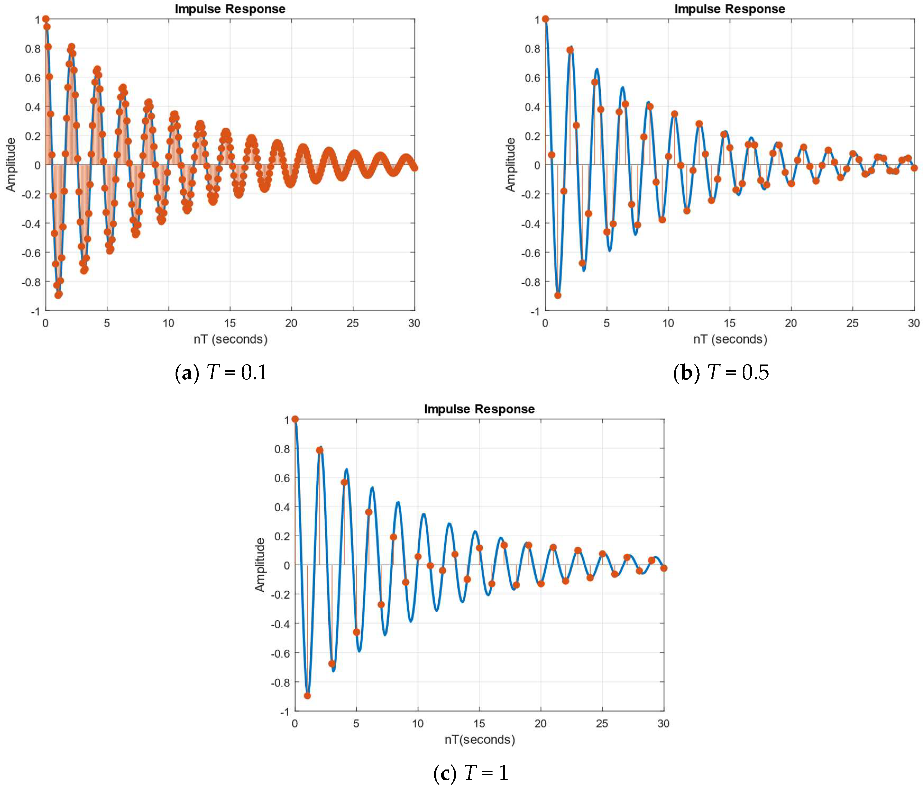
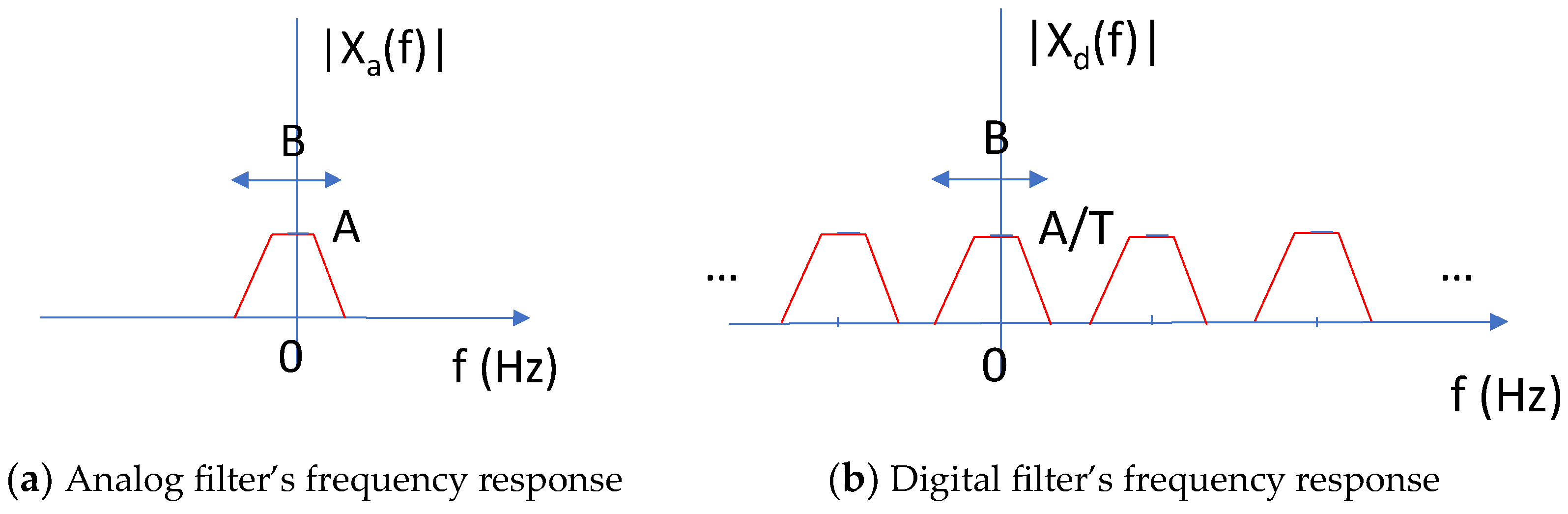
2.1. Impulse Invariance Filter (IIF) Design

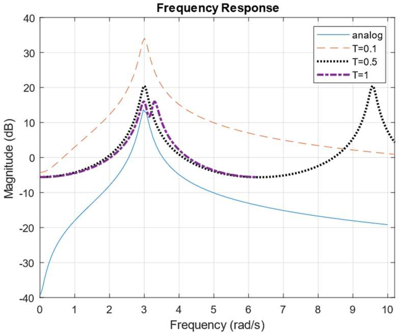
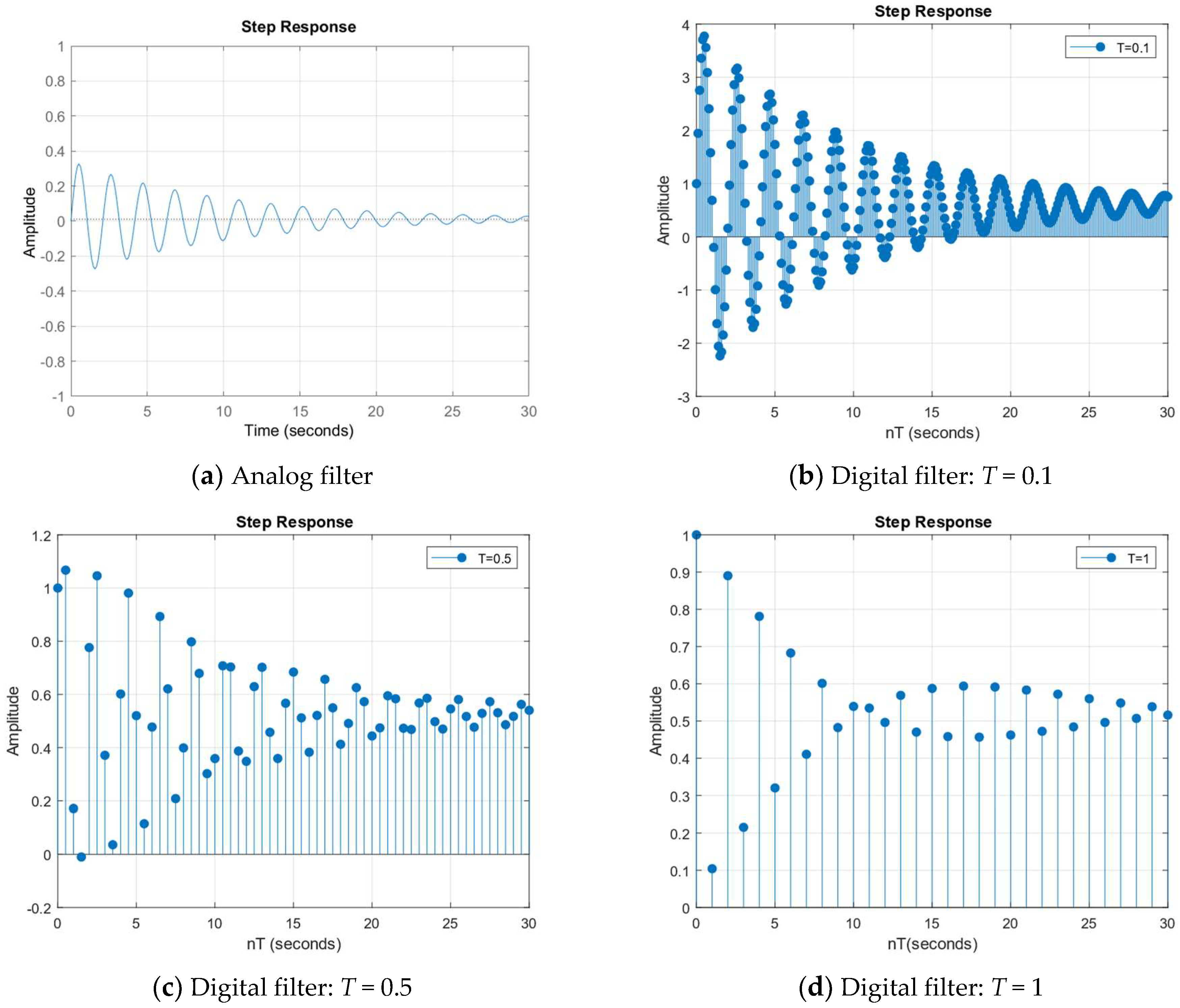
For digital IIR filters, one popular category of design technique is to convert well-designed analog filters to digital filters. In this category, there are several techniques, including IIR filter design using approximation of derivatives, IIR filter design by impulse invariance, IIR filter design using matched poles and zeros, and IIR filter design by bilinear transformation. See [1,19] for details.

Here, the IIF design procedures are briefly reviewed. Given a well-designed analog filter transfer function H_a(s) whose impulse response is represented as h_a(t) and its sampled impulse response is denoted by

h(n) = h_a(nT),   n = 0, 1, 2, 3, ….

(1)

where T is the sampling interval.

When a continuous signal h_a(t) with spectrum $H_a\left(\omega \right)$ is sampled with a sampling interval T or a sampling rate of $F_s={\displaystyle \frac{1}{T}}$, the spectrum of the sampled signal/digital filter with sample response h(n) = h_a(nT) has the following frequency response [1]:

$$H\left(f\right)=F_s{\sum }_{-\infty }^{\infty }{H}_a\left((f-k{F}_s)\right)$$

(2)

or

$$H\left(\omega \right)=F_s{\sum }_{-\infty }^{\infty }{H}_a\left((\omega -2\pi k{F}_s)\right)$$

(3)

or

$$H\left(\mathsf{\Omega }\mathrm{T}\right)=F_s{\sum }_{-\infty }^{\infty }{H}_a\left((\mathsf{\Omega }-{\displaystyle \frac{2\pi k}{T}})\right)$$

(4)

where $f=F/F_s$, $\omega =2\pi f$, $\mathsf{\Omega }=2\pi F,$ and $\omega =\mathsf{\Omega }\mathrm{T}$. Details can be found in [1].

To visualize Equations (2)–(4), one can look at Figure 10.3.3 in [1], in which one can see that the digital filter response H(f) is a periodic replica of the analog spectral response H_a(f).

In terms of s- and z-transforms, the relationship between the digital filter and the analog filter is given by [1]:

$$H\left(\mathrm{z}\right)={\displaystyle \frac{1}{T}}{\sum }_{-\infty }^{\infty }{H}_a\left((\mathrm{s}-j{\displaystyle \frac{2\pi k}{T}})\right)$$

(5)

where

$$H\left(\mathrm{z}\right)={\sum }_{n=0}^{\infty }h\left(n\right)z^{-n}$$

(6)

$$\mathrm{z}=e^{sT}$$

(7)

Without loss of generality, the case where the poles of the analog filter are distinct is considered here. The following materials are summarized from [1]. For repeated poles, the design can still proceed by including more terms associated with the higher order terms in the partial fraction expansion. The analog filter using partial fraction expansion is then given by

$$H_a\left(s\right)={\sum }_{k=1}^N{\displaystyle \frac{c_k}{s-p_k}}$$

(8)

where $p_k$ are the poles and $c_k$ are the coefficients of the partial fraction expansion. The impulse response can be obtained as

$$h_a\left(t\right)={\sum }_{k=1}^N{c}_k{e}^{p_{k}t}, t\ge 0$$

(9)

If one samples $h_a\left(t\right)$ at t = nT, then the discretized impulse response is

$$h\left(n\right)=h_a\left(\mathit{nT}\right)={\sum }_{k=1}^N{c}_k{e}^{p_{k}nT}$$

(10)

Substituting (10) into (6), the digital IIR filter obtained by the impulse invariance design procedure is then given by

$$H\left(z\right)={\sum }_{n=0}^{\infty }h\left(n\right)z^{-n}={\sum }_{n=0}^{\infty }{\displaystyle \frac{c_k}{1-e^{p_{k}T}{z}^{-1}}}$$

(11)

Comparing $H_a\left(s\right)$ in (8) and $H\left(z\right)$ in (11), one can see that the analog poles are mapped to the digital filter poles via

$$z_k=e^{p_{k}T},\hspace{1em}\hspace{1em}k=1,2,\dots ,N$$

(12)

2.2. Issues

Earlier, it was mentioned that if one strictly follows the IIF design procedures, then there will be some confusing issues. Let us use Example 10.3.3 in Proakis and Manolakis’ book [1] to illustrate the issues.

Equation (13) below shows the desired analog filter, which is a bandpass filter, that needs to be converted to a digital filter.

$$H_a\left(s\right)={\displaystyle \frac{s+0.1}{{(s+0.1)}^2+9}}$$

(13)

Following the IIF design procedures described in Section 2.1, the digital filter’s impulse response is the sampled version of the analog filter’s impulse response. The resulting digital filter is given by Equation (14).

$$H_1\left(z\right)={\displaystyle \frac{1-\left({\mathrm{e}}^{-0.1T}\mathrm{c}\mathrm{o}\mathrm{s}3T\right)z^{-1}}{1-\left({2\mathrm{e}}^{-0.1T}\mathrm{c}\mathrm{o}\mathrm{s}3T\right)z^{-1}+{\mathrm{e}}^{-0.2T}{z}^{-2}}}$$

(14)

Figure 1 shows the impulse responses of the analog filter and digital filter with different sampling periods of T (T = 0.1, 0.5, 1) seconds. It can be clearly seen that the impulse responses of the analog and digital filters match. Next, the frequency responses of the analog and digital filters are plotted in Figure 2. Figure 3 shows the step responses of the analog and digital filters. From Figure 2 and Figure 3, the first issue is that one can clearly see that the digital filters’ responses are 1/T times larger than that of the analog filter. The second issue is that one can see that the digital filters’ step responses not only do not look similar to the analog filter’s output but also have different steady state responses. From the above observations, it can be concluded that constraining the digital filter’s impulse response to be exactly the same as the analog’s impulse response is not a good design principle because the resulting digital filter differs from the analog filter in both frequency and step responses. In both the frequency and step responses, the amplitudes differ by a factor of 1/T.

2.3. Remedies to Resolve the Inconsistency Issues in Frequency and Step Responses

Now, two remedies will be presented. Remedy 1 can resolve the inconsistencies in both the frequency and step responses. Remedy 2 can also resolve both inconsistencies in frequency and step responses. However, the impulse responses of the analog and digital filters do not match each other anymore in Remedy 2.

2.3.1. Remedy Method 1: Scale the Digital Filter Frequency and Step Responses by T

One can call Remedy 1 a post-processing step after the filter has been designed using the standard IIF design procedures.

To explain the behavior of the frequency response in Figure 2, the answer can be found by looking at Equation (5). From Equation (5), one can see that the digital filter response is 1/T times the analog filter response.

In order to match the analog and digital filter frequency responses, one simple remedy is to scale the digital filter frequency response by multiplying it with the sampling interval T. The justification for this method is that the relationship between the analog and digital filters’ frequency responses due to sampling operations can be illustrated in Figure 4. It can be clearly seen that the amplitude of the frequency response of the digital filter is 1/T times that of the analog filter. Because of the above scaling effect, the output of the digital filter will be scaled by 1/T. Hence, one should multiply the output of the digital filter by T in order to obtain the same results as the analog filter’s output.

Using the same example (originally from [1]) as in Section 2.2, one can multiply the frequency response in Figure 2 by T and then obtain Figure 5 below. It can be seen that for T = 0.1 and T = 0.5, the frequency responses of the analog and digital filters match quite well over a frequency range of 1 to 5 rad/s. For the step response, one can multiply the step responses in Figure 3 by T, and the resulting step responses are shown in Figure 6. One can observe that the step responses of the analog and digital filter are similar, especially for small Ts. Note that the performance of impulse invariance filter design depends on the sampling interval T. A smaller T gives better matching results. For large Ts, frequency and step responses of the digital filter differ more from the analog filter responses.

Hence, if one directly uses the sampled analog filter impulse response as the digital filter impulse response, then one should remember to scale the digital filter’s step response and frequency response by multiplying by the sampling period T. Otherwise, the analog and digital filter responses will have a scaling difference of 1/T.

2.3.2. Remedy Method 2: Scale the Impulse Response by T

In Remedy 1, it is recommended to scale the digital filter frequency and step responses by multiplying by the sampling period T. Here, a pre-processing approach is presented, which was mentioned in [2], where the sampled analog’s impulse response is multiplied by T to obtain the digital filter impulse response. The digital filter’s outputs will then be the same as the analog filter’s frequency and step responses. The results are the same as those in Figure 5 and Figure 6. Hence, those responses are not replicated here.

Mathematically, since the frequency response of the analog filter $H_a(\omega$) is related to its impulse response via the Fourier Transform (linear),

$$H_a\left(\omega \right)={\int }_{-\infty }^{\infty }{h}_a\left(t\right)e^{-j\omega t}dt.$$

(15)

If one discretizes (15), then one will obtain an approximate frequency response $H_d\left(\omega \right)$:

$$H_d\left(\omega \right)={\sum }_{-\infty }^{\infty }h\left(nT\right)e^{-j\omega nT}T={\sum }_{-\infty }^{\infty }Th\left(nT\right)e^{-j\omega nT} .$$

(16)

From Equation (7), the digital filter response $H\left(\omega \right)$ will be the same as $H_d\left(\omega \right)$ if one defines h(n) = $Th\left(nT\right)$ in Equation (16).

Hence, the idea of Remedy 2 is to scale the analog impulse response by T and use the scaled version as the impulse response for the digital filter. Here, using the same example as earlier, the digital filter is given by

$$H_2\left(z\right)=T{H}_1\left(z\right)={\displaystyle \frac{T(1-\left( e^{-0.1T}\mathrm{c}\mathrm{o}\mathrm{s}3T\right)z^{-1})}{1-\left({2e}^{-0.1T}\mathrm{c}\mathrm{o}\mathrm{s}3T\right)z^{-1}+e^{-0.2T}{z}^{-2}}}$$

(17)

Strictly speaking, Remedy 2 or the alternative method mentioned in [2] should be called a modified impulse invariance method because the analog impulse response and the digital impulse response are no longer the same. Figure 7 compares the impulse responses of the analog and digital filters. It can be seen that the digital filters’ impulse responses are scaled by T times the analog response.

However, the steady state values of step responses for the digital filter shown in Figure 6 are different from the analog filter. Smaller Ts have smaller biases. In Section 2.3 below, the reason for the biases will be explained.

2.4. An Improved IIF Design

In Section 2.3, the modified IIF design (Remedy 2) resolves the matching issues in both the frequency and step responses. However, the existence of steady state errors is prominent in the step responses. Some minor differences between the analog and digital filter outputs can be seen from Figure 6. Based on the subplots Figure 6b–d, one can intuitively link those differences to the digital sampling period T because, for smaller Ts, one can still observe small biases. The reason is because of the discontinuity at t = 0 in the analog filter’s impulse response.

In a paper by Jackson [3], it was pointed out that, for rational analog filters with a relative degree difference of one, there is a discontinuity at t = 0 in the impulse response. Due to this discontinuity, the modified impulse invariance method mentioned in Section 2.3 (Remedy 2) should have an additional correction term in order to avoid some biases between analog and digital filter responses. Details can be found in [5]. Specifically, for an analog filter of the form

$$H_a\left(s\right)={\sum }_{k=1}^N{\displaystyle \frac{A_k}{s-p_k}},$$

(18)

the corrected digital filter based on the modified impulse invariance method is given by

$$H\left(z\right)={\sum }_{k=1}^N{\displaystyle \frac{T{A}_k}{1-e^{p_k}{z}^{-1}}}-{\displaystyle \frac{T}{2}}{\sum }_{k=1}^N{A}_k.$$

(19)

The same example to illustrate this improved IIF design will be used below.

Following the recommendation described in [5], a correction term mentioned in Equation (19) is added into Equation (17). Now, the improved digital filter becomes

$$H_3\left(z\right)=H_2\left(z\right)-{\displaystyle \frac{T}{2}}={\displaystyle \frac{T(1-\left(e^{-0.1T}\mathrm{c}\mathrm{o}\mathrm{s}3T\right)z^{-1})}{1-\left({2e}^{-0.1T}\mathrm{c}\mathrm{o}\mathrm{s}3T\right)z^{-1}+e^{-0.2T}{z}^{-2}}}-T/2$$

(20)

Comparing Figure 7 and Figure 8, one can see that the correction term in (9) has negligible impact in the impulse response (Figure 8). However, comparing Figure 5 and Figure 9, the frequency responses of the digital filters with the correction term are much closer to the analog filter’s response. Similarly, comparing Figure 6 and Figure 10, the small biases are much smaller in the step responses of the digital filters with the correction term.

Hence, Equation (19) is the recommended IIF design procedure.

3. Additional Examples

3.1. Example 1: Lathi and Green’s Example 5.16 [2]

Here, three impulse invariance filter designs using Example 5.16 in Lathi and Green’s textbook [2] will be summarized. The analog filter is a simple lowpass filter given by Equation (21):

$$H_a\left(s\right)={\displaystyle \frac{{\omega }_c}{s+{\omega }_c}}$$

(21)

where ${\omega }_c={10}^5$.

3.1.1. Traditional Impulse Invariance Design (Section 2.1)

Assuming a sampling period T and imposing the same impulse responses in the analog and digital filters, the digital filter is given by

$$H_1\left(z\right)={\displaystyle \frac{{\omega }_c}{1-e^{-{\omega }_{c}T}{z}^{-1}}}$$

(22)

Figure 11 shows that all impulse responses are the same, aligning with the design principle. Three different Ts were used. However, Figure 12 shows that the frequency responses of the digital filters are different from that of the analog response. From Figure 13, one can see that the step responses of the analog and digital filters are also different. This means that imposing the exact impulse responses on both analog and digital filters is inappropriate and can cause completely different frequency and step responses between the analog and digital filters. One remedy is to scale the frequency response and step response of the digital filters by T.

3.1.2. Modified Impulse Invariance Design (Remedy 2 in Section 2.3)

Instead of scaling the output and frequency response by T, an alternative method is to scale the impulse response of the analog filter by T and then use the scaled version as the impulse response of the digital filter. If one does that, the resulting digital filter becomes

$$H_2\left(z\right)=T{H}_1\left(z\right)={\displaystyle \frac{T{\omega }_c}{1-e^{-{\omega }_{c}T}{z}^{-1}}}.$$

(23)

Figure 14 plots all the impulse responses. Although the impulse responses of the digital filters are not same as the analog one, the frequency and step responses of the digital filters are much closer to the analog responses, as shown in Figure 15 and Figure 16, respectively. One can observe that there are some steady state biases between the analog and digital filter outputs. The magnitude of the biases is proportional to T.

3.1.3. Improved Impulse Invariance Design with a Correction Term

The biases in Figure 16b–d can be reduced if one includes a correction term in the digital filter. The resulting filter is then given by

$$H_3\left(z\right)={\displaystyle \frac{T{\omega }_c}{1-e^{-{\omega }_{c}T}{z}^{-1}}}-T{\omega }_c/2$$

(24)

Although the impulse responses are not the same between the analog and digital filters, as seen in Figure 17, the frequency responses and step responses in Figure 18 and Figure 19 are much closer between the analog and digital filters. Most importantly, the biases in the step responses are reduced to almost zero.

3.2. Example in Jackson’s Paper [3]

The analog filter shown in Equation (25) is a resonant filter (bandpass filter):

$$H_a\left(s\right)={\displaystyle \frac{2as}{{(s+a)}^2+{\mathsf{\Omega }}_0^2}}$$

(25)

where a = 2 and ${\mathsf{\Omega }}_0=10.$ Assuming a sampling period T = 0.1, by imposing the same impulse response in the analog and digital filters, a direct/traditional impulse invariance design will yield the following digital filter:

$$H_1\left(z\right)={\displaystyle \frac{2a\left(1-r\mathrm{c}\mathrm{o}\mathrm{s}\left({\omega }_0\right)z^{-1}\right)-2a^2/{\mathsf{\Omega }}_0\left(r\mathrm{s}\mathrm{i}\mathrm{n}\left({\omega }_0\right)\right)z^{-1}}{1-2r\mathrm{c}\mathrm{o}\mathrm{s}\left({\omega }_0\right)z^{-1}+r^2{z}^{-2}}}$$

(26)

where $r=e^{-aT}$ and ${\omega }_0={\mathsf{\Omega }}_{0}T$. The digital filter designed using the modified impulse invariance method is given by

$$H_2\left(z\right)={\displaystyle \frac{2aT\left(1-r\mathrm{c}\mathrm{o}\mathrm{s}\left({\omega }_0\right)z^{-1}\right)-2aTa/{\mathsf{\Omega }}_0\left(r\mathrm{s}\mathrm{i}\mathrm{n}\left({\omega }_0\right)\right)z^{-1}}{1-2r\mathrm{c}\mathrm{o}\mathrm{s}\left({\omega }_0\right)z^{-1}+r^2{z}^{-2}}}.$$

(27)

Using the improved impulse invariance method with correction term (Equation (19)), one has

$$H_3\left(z\right)=H_2\left(z\right)-aT$$

(28)

Figure 20 compares the impulse responses of the analog and digital filters. $H_1$ is similar to the analog filter, whereas $H_2$ and $H_3$ are different. However, from Figure 21, $H_3$ has the closest frequency response to the analog filter. Also, from the step responses shown in Figure 22, $H_3$ has the closest response to the analog filter. $H_1$ differs the most from the analog filter’s step response.

4. MATLAB R2021a’s Impinvar Command Using the Modified Impulse Invariance Method without a Correction Term

MATLAB R2021a’s impinvar is using the modified impulse invariance method (Remedy 2), but there is no correction term. This fact was not explicitly stated in MATLAB R2021a’s help menu. The following example is employed to validate the preceding statement.

Example 3: Apply MATLAB R2021a’s Impinvar Command to Equation (21)

Using the MATLAB R2021a impinvar command, one will get

• >> omegac = 10⁵; Ba = [omegac]; Aa = [1 omegac]; Fs = 10⁶/pi;
• >> [B,A] = impinvar(Ba,Aa,Fs)
• B = 0.3142
• A = 1.0000−0.7304; % without correction term

In other words, the digital filter using impinvar is given by

$$H_1\left(z\right)={\displaystyle \frac{0.3142}{1-0.7304z^{-1}}}.$$

(29)

Equation (29) is the same as Equation (23), which is the filter designed by Remedy 2 or the modified impulse invariance filter design. If the correction term is included, the following filter is obtained:

$$H_2\left(z\right)={\displaystyle \frac{0.3142}{1-0.7304z^{-1}}}-{\displaystyle \frac{T{\omega }_c}{2}}={\displaystyle \frac{0.3142}{1-0.7304z^{-1}}}-0.01/\pi$$

(30)

The frequency response of the filter (with correction term) in Equation (30) is compared with the filter using impinvar in Equation (29) without correction term. The result shown in Figure 23 concludes that the impinvar filter indeed does not contain the correction term.

In addition, it is recommended to include a correction term to the impinvar filter so that both the step and frequency responses of the digital filter will be close to the analog filter.

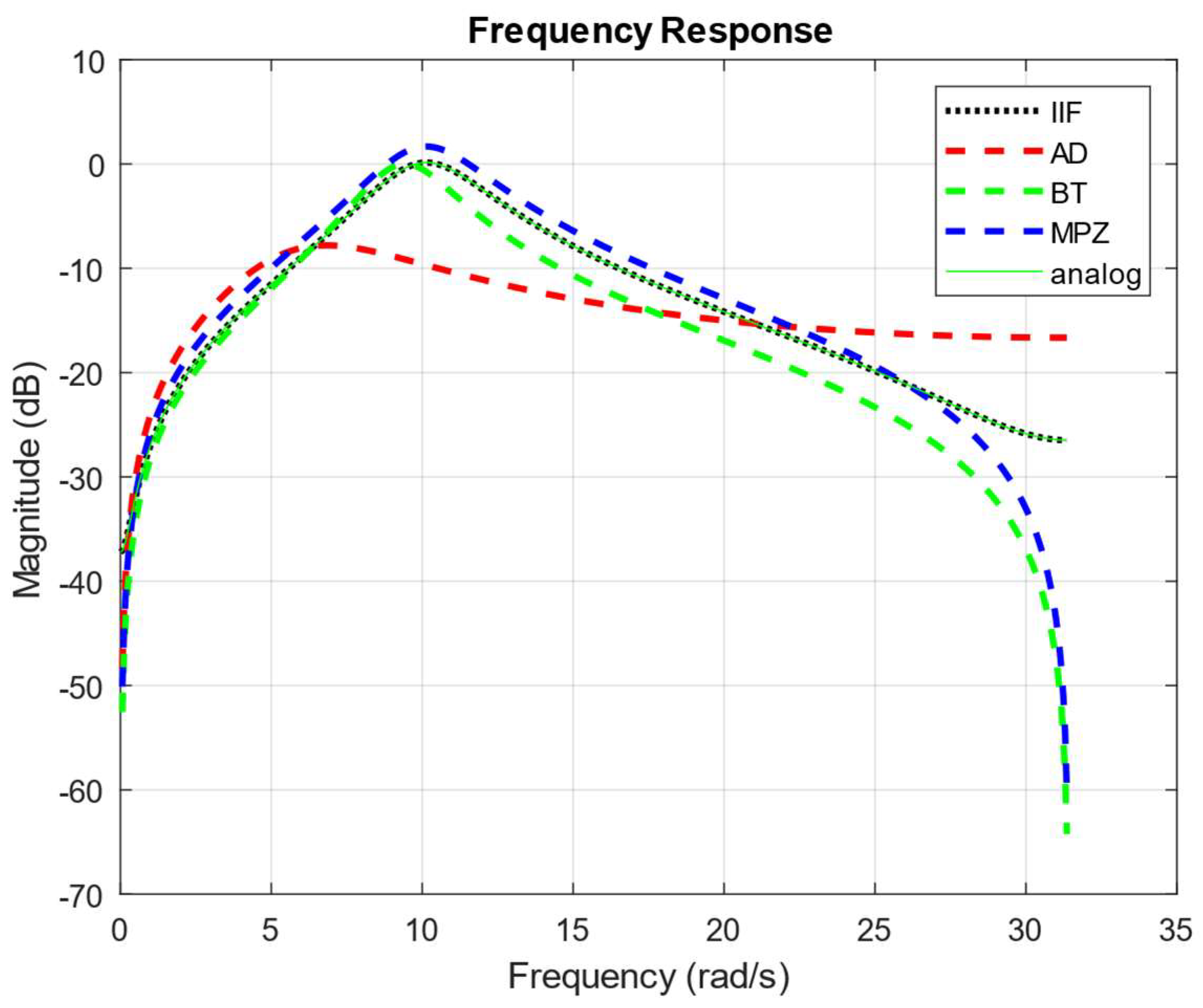
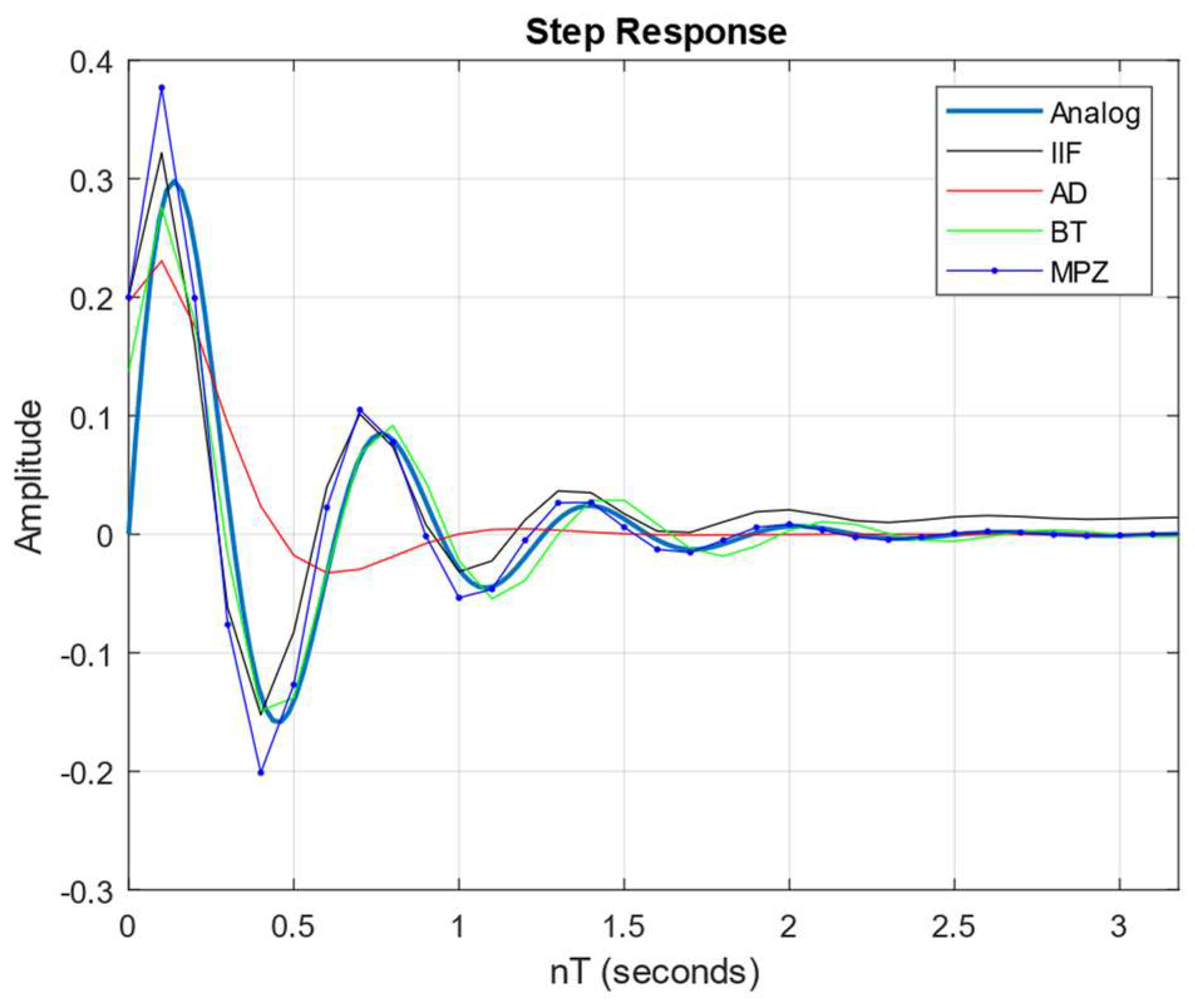
5. Comparative Studies with Three Well-Known Digital IIR Filter Design Techniques

Here, we focus on the comparison of the improved IIF with three well-known digital IIR filter design techniques. One is called the approximation of derivatives (AD) [1] and the second is the bilinear transformation (BT) [1]. The third one is the matched pole zero (MPZ) filter design, which is very popular in digital control [23].

5.1. Comparative Study 1

We repeat the analog filter given by Equation (21) here:

$$H_a\left(s\right)={\displaystyle \frac{{\omega }_c}{s+{\omega }_c}}$$

(31)

where ${\omega }_c={10}^5$.

Using the AD method described in [1], we substitute the variable s in Equation (31) with $s={\displaystyle \frac{1-z^{-1}}{T}}$ to get the digital IIR filter

$$H_{AD}\left(z\right)={\displaystyle \frac{{\omega }_{c}T}{1+{\omega }_{c}T-z^{-1}}}$$

(32)

Using the BT technique, we substitute the variable s in Equation (31) by $s={\displaystyle \frac{2}{T}}{\displaystyle \frac{1-z^{-1}}{1+z^{-1}}}$ to get the digital IIR filter

$$H_{BT}\left(z\right)={\displaystyle \frac{{\omega }_c(1+z^{-1})}{\left(\frac{2}{T}+{\omega }_c\right)+({\omega }_c-\frac{2}{T})z^{-1}}}.$$

(33)

Using the MPZ technique, we substitute each pole and zero with $z=e^{-sT}$ to get a digital filter of the form

$$H_{MPZ}\left(z\right)={\displaystyle \frac{(1-e^{-{\omega }_{c}T})(1+z^{-1})}{2(1-e^{-{\omega }_{c}T}{z}^{-1})}}$$

(34)

Now, we can compare the time and frequency domain responses of IIF in Equation (24), AD in Equation (32), BT in Equation (33), and MPZ in Equation (34) for two Ts (10⁻⁶, 2 × 10⁻⁶). Figure 24 compares the impulse responses of the four filters for T = 10⁻⁶ s. All have similar responses except for the AD method. Figure 25 compares the frequency responses of the four digital filters with the analog filter for T = 10⁻⁶ s. It is observed that the IIF and BT responses overlap on top of each other. AD and MPZ show big differences from the analog response. Figure 26 compares the step responses for T = 10⁻⁶ s. All filters have similar responses.

Now, we show results for T = 2 × 10⁻⁶ s. Figure 27 compares the impulse responses. MPZ has the worst performance and the others have a similar performance. Figure 28 shows the frequency responses, and one can see that AD and MPZ have a poor performance as compared with the IIF and BT methods. Figure 29 shows the step responses of the various filters. The responses all look similar.

5.2. Comparative Study 2

We repeat the resonant filter (bandpass filter) below:

$$H_a\left(s\right)={\displaystyle \frac{2as}{{(s+a)}^2+{\mathsf{\Omega }}_0^2}}$$

(35)

where a = 2 and ${\mathsf{\Omega }}_0=10,$ and the sampling period T = 0.1.

Using the AD method described in [1], we substitute the variable s in Equation (35) by $s={\displaystyle \frac{1-z^{-1}}{T}}$ to get the digital IIR filter

$$H_{AD}\left(z\right)={\displaystyle \frac{2aT(1-z^{-1})}{1+{(a}^2+{\mathsf{\Omega }}_0^2)T^2-2\left(1+aT\right)z^{-1}+z^{-2}}}$$

(36)

Using the BT technique, we substitute the variable s in Equation (35) by $s={\displaystyle \frac{2}{T}}{\displaystyle \frac{1-z^{-1}}{1+z^{-1}}}$ to get the digital IIR filter

$$H_{BT}\left(z\right)={\displaystyle \frac{4aT(1-z^{-2})}{\left[{(2+aT)}^2+{\mathsf{\Omega }}_0^2{T}^2\right]+2\left[\left(2+aT\right)\left(aT-2\right)+{\mathsf{\Omega }}_0^2{T}^2\right]z^{-1}+[{\left(aT-2\right)}^2+{\mathsf{\Omega }}_0^2{T}^2]z^{-2}}}.$$

(37)

Using the MPZ technique, we substitute each pole and zero with $z=e^{-sT}$ to get a digital filter of the form

$$\begin{gathered} H_{MPZ}\left(z\right)={\displaystyle \frac{2a\left(1-z^{-2}\right)}{\left[1-e^{-\left(a+j{\mathsf{\Omega }}_0\right)T}{z}^{-1}\right]\left[1-e^{-\left(a-j{\mathsf{\Omega }}_0\right)T}{z}^{-1}\right]}} \\ ={\displaystyle \frac{2a\left(1-z^{-2}\right)}{1-2e^{-aT}\cos \left({\mathsf{\Omega }}_{0}T\right)z^{-1}+e^{-2aT{z}^{-2}}}} \end{gathered}$$

(38)

Now we can compare the time and frequency domain responses of IIF in Equation (28), AD in Equation (36), BT in Equation (37), and MPZ in Equation (38) for T = 0.1 s. Figure 30 compares the impulse responses. One can see that all of the digital filters have similar responses. Figure 31 is an important figure, which clearly illustrates the benefit of IIF. One can see that the IIF response overlaps with the analog response across the frequency range of interest. BT performs the second best. AD and MPZ have moderately large differences as compared to the analog response. Figure 32 shows the step responses. One can see that IIF has a small bias. However, this bias would have been much bigger without the correction term shown in Equation (28).

It is important to emphasize that the most important feature of digital filters is the frequency response because the goal of a digital filter is to filter out uncertain signals. If a digital filter can match the corresponding analog filter’s frequency response, then it is a good design. With respect to this feature, IIF clearly shows a key advantage over the other three competing methods.

5.3. Remarks

Here, we include a few notes about filter choices and errors related to large sampling periods:

• Applicability of IIF
  As noted by Oppenheim and Schafer in 1975 [19], IIF is most suitable for bandlimited applications, such as lowpass and bandpass filters. For applications requiring highpass filtering, bilinear transformation (BT) or other methods may be more appropriate.

• Scaling and Bias Term

  ○

  Scaling: The scaling issue is relevant to all IIF filters and should be addressed to ensure accurate filter design.

  ○

  Bias Term: The correction for the bias term is necessary primarily for IIF filters with a relative degree of one where discontinuities in the impulse response occur. For filters with a relative degree greater than one, the bias term is generally not required because the initial value theorem ensures that the initial impulse response value is zero.

• Importance of Correct Filter Design
  In order to select the best filter for an application, one needs to assess several available filters in the literature. If one filter has some inherent issues, such as the IIF without the bias term, then one may easily eliminate the IIF and select other filters. For example, in the second case study in our paper, if the IIF filter is used in the comparison without adding the bias term, then the IIF will be eliminated in the trade-off studies and another filter will be chosen instead. Hence, it is critical to have the correct filters in order to choose the right filter for a given application.

• Mathematical Analysis of Errors
  It will be important to provide a detailed mathematical analysis of the errors introduced by the correction term, especially for a larger sampling interval T. Jackson’s paper [3] did address this issue, providing a mathematical expression for the error term, which highlights that the contribution of the bias term increases with the sampling period T. In particular, the mathematical expression from Jackson’s paper is as follows:

  $$H\left(z\right)={\sum }_{k=1}^N{\displaystyle \frac{T{A}_k}{1-e^{p_k}{z}^{-1}}}-{\displaystyle \frac{T}{2}}{\sum }_{k=1}^N{A}_k,$$

  which is actually Equation (19) in our paper. We can see that the last term $-{\displaystyle \frac{T}{2}}{\sum }_{k=1}^N{A}_k$ shows the contribution of the bias term, which is proportional to the sampling period T. Larger Ts will give larger errors in the frequency response.

6. Conclusions

In IIR filter design, engineers frequently show confusion relating to certain aspects of impulse invariance filter (IIF) design. For instance, if one constrains the analog and digital filters to have the same impulse response, then the frequency response and outputs of the analog and digital filters will be different by a scaling factor. If one scales the impulse response of the analog filter by T and makes the scaled impulse response the same as that of the digital filter, then the frequency response and filter outputs will be close, but still not the same in some cases. It was pointed out that if the analog filter’s relative degree difference is one, then a correction term will need to be added in the digital filter transfer function. Moreover, it was highlighted that the MATLAB R2021a command impinvar does not have a correction term and hence will show some slight differences between the analog and digital filter frequency responses. Finally, comparative studies with four digital IIR filter design techniques were carried out. It was observed that the improved IIF design has a comparable or better performance than other competing methods, especially in frequency response. Examples were provided to help engineers and practitioners understand these issues and come up with more accurate digital filter designs.

References

1. Proakis, J.; Manolakis, D.G. Digital Signal Processing, 5th ed.; Pearson: London, UK, 2021. [Google Scholar]
2. Lathi, B.P.; Green, R. Linear Systems and Signals, 3rd ed.; Oxford University Press: Oxford, UK, 2018. [Google Scholar]
3. Jackson, L.B. A correction to impulse invariance. IEEE Signal Process. Lett. 2000, 7, 273–275. [Google Scholar] [CrossRef]
4. Shiung, D.; Huang, J.-J.; Yang, Y.-Y. Tricks for Designing a Cascade of Infinite Impulse Response Filters with an Almost Linear Phase Response [Tips & Tricks]. IEEE Signal Process. Mag. 2023, 40, 64–73. [Google Scholar]
5. Jain, N.; Rathore, S.; Singh, S.K. Designing and Evaluation of the Reduced Order IIR Filter Design for Signal De-Noising. In Proceedings of the 10th IEEE International Conference on Communication Systems and Network Technologies (CSNT), Bhopal, India, 24–25 April 2021; pp. 375–380. [Google Scholar]
6. Kwan, H.K.; Zhang, M. IIR Filter Design Using Multi-Objective Teaching-Learning-Based Optimization. In Proceedings of the 2018 IEEE Canadian Conference on Electrical & Computer Engineering (CCECE), Quebec, QC, Canada, 13–16 May 2018; pp. 1–4. [Google Scholar]
7. Pal, R. Comparison of the design of FIR and IIR filters for a given specification and removal of phase distortion from IIR filters. In Proceedings of the International Conference on Advances in Computing, Communication and Control (ICAC3), Mumbai, India, 1–2 December 2017; pp. 1–3. [Google Scholar]
8. Zahradnik, P. Closed-form design of optimal equiripple FIR filters. In Proceedings of the 2nd International Conference on Telecommunication and Networks (TEL-NET), Noida, India, 10–11 August 2017. [Google Scholar]
9. Nagahara, M. Min-Max Design of FIR Digital Filters by Semidefinite Programming. 2013. Available online: http://arxiv.org/abs/1308.2013v1 (accessed on 17 September 2024).
10. Boyaci, O.; Narimani, M.R.; Davis, K.; Serpedin, E. Infinite Impulse Response Graph Neural Networks for Cyberattack Localization in Smart Grids. 2022. Available online: http://arxiv.org/abs/2206.12527v1 (accessed on 17 September 2024).
11. Kennedy, H.L. Digital Filters with Vanishing Moments for Shape Analysis. 2019. Available online: http://arxiv.org/abs/1912.07133v4 (accessed on 17 September 2024).
12. Kennedy, H.L. Digital Filter Designs for Recursive Frequency Analysis. 2014. Available online: http://arxiv.org/abs/1408.2294v3 (accessed on 17 September 2024).
13. Valderrama-Cuervo, J.C.; López-Parrado, A. Open Cores for Digital Signal Processing. 2014. Available online: http://arxiv.org/abs/1402.6005v1 (accessed on 17 September 2024).
14. Raju, M.H.; Friedman, L.; Bouman, T.M.; Komogortsev, O.V. Filtering Eye-Tracking Data from an EyeLink 1000: Comparing Heuristic, Savitzky-Golay, IIR, and FIR Digital Filters. 2023. Available online: http://arxiv.org/abs/2303.02134v1 (accessed on 17 September 2024).
15. Kennedy, H.L. Recursive and Non-recursive Filters for Sequential Smoothing and Prediction with Instantaneous Phase and Frequency Estimation Applications (Extended Version). 2023. Available online: http://arxiv.org/abs/2311.07089v3 (accessed on 17 September 2024).
16. Vargas, R.A.; Burrus, C.S. Iterative Design of Lp Digital Filters. 2012. Available online: http://arxiv.org/abs/1207.4526v1 (accessed on 17 September 2024).
17. Kumar, V.; Bhooshan, S. Design of One-Dimensional Linear Phase Digital IIR Filters Using Orthogonal Polynomials. 2013. Available online: http://arxiv.org/abs/1307.2817v1 (accessed on 17 September 2024).
18. Carrasco, J.; Heath, W.P.; Ahmad, N.S.; Wang, S.; Zhang, J. Convex Searches for Discrete-Time Zames-Falb Multipliers. 2018. Available online: http://arxiv.org/abs/1812.02397v1 (accessed on 17 September 2024).
19. Oppenheim, A.V.; Schafer, R.W. Digital Signal Processing, 1st ed.; Pearson: London, UK, 1975. [Google Scholar]
20. Mecklenbräuker, W.F. Remarks on and correction to the impulse invariant method for the design of IIR digital filters. Signal Process. 2000, 80, 1687–1690. [Google Scholar] [CrossRef]
21. Gabel, R.A.; Roberts, R.A. Signals and Linear Systems; Wiley: New York, NY, USA, 1987; pp. 408–422. [Google Scholar]
22. Lyons, R.G. Understanding Digital Signal Processing, 3rd ed.; Prentice Hall: Hoboken, NJ, USA, 2011. [Google Scholar]
23. Lewis, F.L. Applied Optimal Control and Estimation; Prentice-Hall: Hoboken, NJ, USA, 1992. [Google Scholar]
Figure 1. Comparison of the impulse responses of the analog and digital filters for T = 0.1, 0.5 and 1. The responses are the same. The continuous curves denote the analog impulse responses. The dots denote the digital filter responses.
Electronics 13 03753 g001
Figure 2. Comparison of the frequency responses of the analog and digital filters. The analog and digital filter responses differ by a scaling factor of 1/T.
Electronics 13 03753 g002
Figure 3. Comparison of step responses of the analog and digital filters. The analog and digital filter outputs differ by a scaling factor of 1/T.
Electronics 13 03753 g003
Figure 4. Illustration of the frequency responses of the analog and digital filters.
Electronics 13 03753 g004
Figure 5. Comparison of the frequency responses of the analog and digital filters. The frequency responses are quite similar to one another. Digital filters with smaller Ts are closer to the analog response.
Electronics 13 03753 g005
Figure 6. Comparison of step responses of the analog and digital filters. There are still small differences between the analog and digital filter responses, especially in the steady state.
Electronics 13 03753 g006
Figure 7. Comparison of the impulse responses of the analog and digital filters. The digital filters’ responses are scaled by T. The continuous curves denote the analog impulse responses.
Electronics 13 03753 g007
Figure 8. Comparison of the impulse responses of the analog and digital filters with correction terms.
Electronics 13 03753 g008aElectronics 13 03753 g008b
Figure 9. Comparison of the frequency responses of the analog and digital filters. The digital filter frequency response with T = 0.1 almost overlaps with the analog response.
Electronics 13 03753 g009
Figure 10. Comparison of step responses of the analog and digital filters. The steady state responses are very close in all filters.
Electronics 13 03753 g010aElectronics 13 03753 g010b
Figure 11. Comparison of the impulse responses of the analog and digital filters. The responses are the same. The continuous curves denote the analog impulse responses.
Electronics 13 03753 g011
Figure 12. Comparison of the frequency responses of the analog and digital filters. The responses differ by a scaling factor of 1/T.
Electronics 13 03753 g012
Figure 13. Comparison of step responses of the analog and digital filters. The outputs differ by a scaling factor of 1/T.
Electronics 13 03753 g013
Figure 14. Comparison of the impulse responses of the analog and digital filters. The responses are not the same. The digital filters’ responses are T times that of the analog’s response.
Electronics 13 03753 g014
Figure 15. Comparison of the frequency responses of the analog and digital filters. Smaller Ts have closer responses to the analog filter’s response.
Electronics 13 03753 g015
Figure 16. Comparison of step responses of the analog and digital filters. Smaller Ts have closer responses to the analog filter’s response.
Electronics 13 03753 g016
Figure 17. Comparison of the impulse responses of the analog and digital filters.
Electronics 13 03753 g017
Figure 18. Comparison of the frequency responses of the analog and digital filters.
Electronics 13 03753 g018
Figure 19. Comparison of step responses of the analog and digital filters.
Electronics 13 03753 g019
Figure 20. Comparison of impulse responses of the analog and digital filters.
Electronics 13 03753 g020
Figure 21. Comparison of frequency responses. H 3 is closer to the analog version than H 2 . H 1 is very different from the analog response.
Electronics 13 03753 g021
Figure 22. Comparison of step responses. H 3 is closer to the analog version than both H 1 and H 2 .
Electronics 13 03753 g022
Figure 23. Comparison of frequency responses. H 2 in Equation (30) is closer to the analog version than H 1 in Equation (21).
Electronics 13 03753 g023
Figure 24. Comparison of the impulse responses of the analog and four digital filters. T = 10−6. BT, IIF, and MPZ have similar responses, but not AD.
Electronics 13 03753 g024
Figure 25. Comparison of the frequency responses of the analog and four digital filters. T = 10−6. IIF and BT overlap on top of each other. AD and MPZ show big differences from the analog response.
Electronics 13 03753 g025
Figure 26. Comparison of step responses of the analog and four digital filters. T = 10−6. All filter responses are similar.
Electronics 13 03753 g026
Figure 27. Comparison of the impulse responses of the analog and four digital filters. T = 2 × 10⁻⁶. IIF and BT overlap on top of each other. AD and MPZ display big differences from the analog response.
Electronics 13 03753 g027
Figure 28. Comparison of the frequency responses of the analog and four digital filters. T = 2 × 10⁻⁶. IIF and BT overlap on top of each other. AD and MPZ have big differences from the analog response.
Electronics 13 03753 g028
Figure 29. Comparison of step responses of the analog and four digital filters. T = 2 × 10⁻⁶. All filter responses are similar.
Electronics 13 03753 g029
Figure 30. Comparison of the impulse responses of the analog and four digital filters. All responses are scaled versions of the analog filter’s response.
Electronics 13 03753 g030
Figure 31. Comparison of the frequency responses of the analog and four digital filters. IIF overlaps with the analog filter response. Other filters’ responses are different from the analog filter response.
Electronics 13 03753 g031
Figure 32. Comparison of the step responses of the analog and four digital filters. All filters follow the analog filter’s response. The IIF has a small bias. However, without correction, the IIF would have a much bigger bias, as shown in Figure 22.
Electronics 13 03753 g032
Disclaimer/Publisher’s Note: The statements, opinions and data contained in all publications are solely those of the individual author(s) and contributor(s) and not of MDPI and/or the editor(s). MDPI and/or the editor(s) disclaim responsibility for any injury to people or property resulting from any ideas, methods, instructions or products referred to in the content.