Abstract
As a compression standard, Geometry-based Point Cloud Compression (G-PCC) can effectively reduce data by compressing both geometric and attribute information. Even so, due to coding errors and data loss, point clouds (PCs) still face distortion challenges, such as the encoding of attribute information may lead to spatial detail loss and visible artifacts, which negatively impact visual quality. To address these challenges, this paper proposes an iterative removal method for attribute compression artifacts based on a graph neural network. First, the geometric coordinates of the PCs are used to construct a graph that accurately reflects the spatial structure, with the PC attributes treated as signals on the graph’s vertices. Adaptive graph convolution is then employed to dynamically focus on the areas most affected by compression, while a bi-branch attention block is used to restore high-frequency details. To maintain overall visual quality, a spatial consistency mechanism is applied to the recovered PCs. Additionally, an iterative strategy is introduced to correct systematic distortions, such as additive bias, introduced during compression. The experimental results demonstrate that the proposed method produces finer and more realistic visual details, compared to state-of-the-art techniques for PC attribute compression artifact removal. Furthermore, the proposed method significantly reduces the network runtime, enhancing processing efficiency.
1. Introduction
A point cloud (PC) is composed of massive irregularly distributed points in 3D space, with each point owning spatial coordinates and associated attributes, such as RGB color, normal, and reflectance. By virtue of their strong flexibility and powerful representation, PCs have been widely implemented in many fields, including autonomous driving [1], 3D immersive visual communication [2], Augmented Reality/Virtual Reality (AR/VR) [3], and Geographic Information Systems (GISs) [4], among others. With the rapid development of 3D sensing and capturing technologies, the volume of PC data has grown in such an explosive manner that a high-quality PC may contain millions of points, or even more. Without proper compression, when transmitted at a rate of 30 frames per second, a single PC containing one million points would take a total bandwidth of 3600 Mbit per second, thus imposing a challenge both in terms of the storage and transmission of PCs. Therefore, the research on PC compression is of great practical significance.
To improve the efficiency of PC compression, the Moving Picture Experts Group (MPEG) has developed two different compression standards [5,6,7,8,9], i.e., Video-based Point Cloud Compression (V-PCC) and Geometry-based Point Cloud Compression (G-PCC), which are used for dense and sparse PCs, respectively. Based on 3D-to-2D projection, the V-PCC [8] standard first divides PCs into multiple 3D blocks, which are then projected onto a 2D plane and packaged into 2D geometric videos and textured videos. Subsequently, these projected videos are compressed using certain well-established video coding standards, such as H.265/High-Efficiency Video Coding [10] (HEVC) or H.266/Versatile Video Coding [11] (VVC). On the other hand, the G-PCC [9] standard compresses PCs directly in 3D space, while treating geometric and attribute information separately. The compression of geometric information is usually based on octree [12,13,14] or mesh/surface methods [15,16]. For the compression of attribute information, hierarchical neighborhood prediction algorithms based on Prediction With Lifting Transform (PredLift) [17,18] and Region-Adaptive Hierarchical Transform (RAHT) [19] have been designed. These compression standards are designed to efficiently compress different types of PCs, so as to meet the needs of various applications.
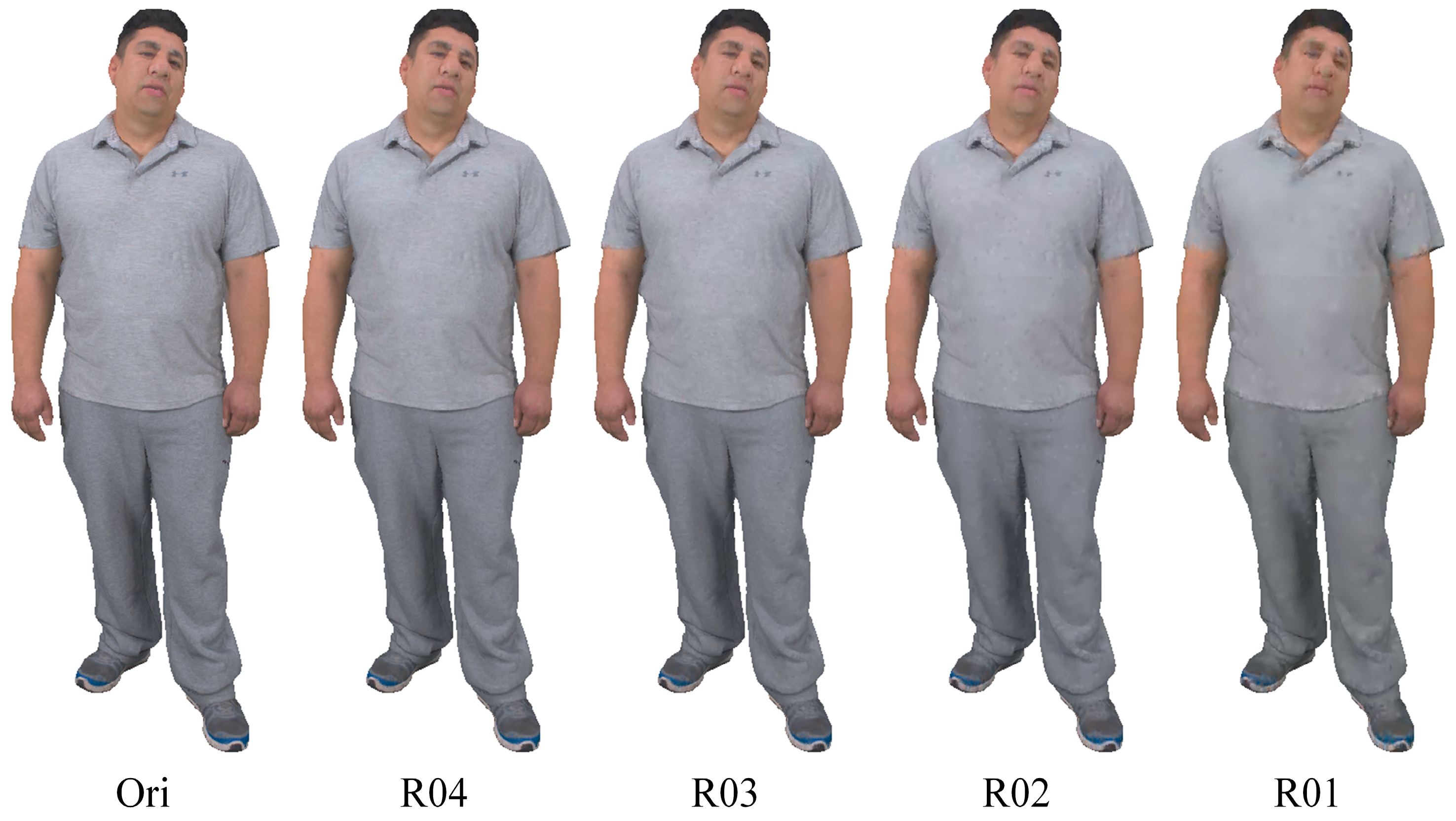
Although the implementation of V-PCC and G-PCC standards has improved the compression efficiency of PCs, the compression process inevitably introduces a variety of compression artifacts, thus compromising the quality of PCs to varying degrees and affecting their fidelity in terms of visual presentation. To further improve the visual quality of PCs in practical applications, it is also crucial to explore and implement effective post-processing techniques; in addition to the commitment to developing and designing more efficient compression methods. Given that the compression artifacts induced by different compression methods vary in regard to the visual characteristics, this paper proposes a post-processing method mainly to address the specific problems concerning attribute compression using the G-PCC standard. Figure 1 demonstrates the PCs after being processed with different G-PCC attribute compression levels, without losing geometric information. As shown in the results, with changes in the compression level, the PCs, to different degrees, present such artifacts as color offset, blurring effect, and striping. These artifacts stem mainly from the information loss during the quantization process. Particularly, the color offset phenomenon is remarkable, which leads to an inconsistency between the color information in the compressed PCs and that of the original PCs. In addition, the blurring effect and striping have significantly reduced the clarity and detail representation of the PCs, compromising the overall visual quality. Hence, this paper tries to explore the method to effectively suppress or repair the above compression artifacts, with a view to significantly boosting the visual fidelity of PCs, while maintaining an efficient compression ratio, to meet the needs of a wider range of applications.
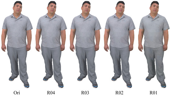
Figure 1.
The “boxer_viewdep_vox12.ply” image [20] under different G-PCC attribute compression levels. First on the left: the original PC, followed by PCs compressed using G-PCC with different attribute compression levels R04, R03, R02, and R01.
Currently, the problems associated with artifacts generated during image and video compression is a widely explored topic, covering the evolution from traditional methods [21,22,23,24,25] to learning-based methods [26,27,28,29,30,31,32,33,34], the application of which has resulted in significant progress in recent years due to the use of models constructed by convolutional operations. However, in nature, convolutional operations rely on spatial continuity between pixels, a feature that does not exist in PCs composed of discrete point sets. As a result, the direct application of such methods in PC processing faces some fundamental challenges. Due to the complexity of PC processing, there is a dearth of post-processing research on the specific attribute artifact problem. For other PC processing tasks, some studies have attempted to convert PCs into projected images [35] or voxels [36,37,38] for representations, to facilitate handling by convolutional neural networks (CNNs). Nevertheless, such conversion methods are often accompanied by the loss of spatial information. In addition, the voxel-based strategy significantly increases the storage and computational burden when dealing with large-scale, high-dimensional data. As a result, such methods encounter limitations in their practical application. Therefore, efficient processing of PCs directly in 3D space has become an appealing research direction. Qi et al. proposed PointNet [39], which can realize end-to-end PC processing, effectively retain the formats of the original data, and successfully achieve feature representation learning. However, PointNet treats each point as an independent unit during processing, while ignoring the proximity and topology between the points, which limits its performance to some extent. For this reason, Qi et al. subsequently proposed PointNet++ [40], which introduced a hierarchical structure to capture the local features of PCs at different levels. Moreover, graph neural networks (GNNs) have achieved impressive results in such tasks as the classification, segmentation, and reconstruction of PCs [41,42,43,44,45,46,47]. By constructing a graph structure, GNNs can effectively capture the local relationships and topologies between points in a PC, thus demonstrating its powerful ability to address the disorderedness and irregularity of PCs.
Based on the above discussion, to address the artifacts commonly found during the attribute compression process involving the G-PCC standard, this paper proposes an iterative removal method for G-PCC attribute artifacts based on a GNN. At the core of this method, it first constructs a graph to characterize the structure of the PC by using the geometric coordinates, and the attribute information is regarded as signals on the vertices of the graph, to realize the deep fusion of spatial and attribute information. Since points may exhibit different distortion degrees due to the influence of artifacts, we adopt the adaptive graph convolution, which aims to accurately capture and extract the feature representation of the attributes of all the points. In particular, more attention is paid to the areas with significant distortions, so as to enhance the sensitivity and accuracy of the artifact recognition. Furthermore, since attribute artifacts often lead to the loss of high-frequency information, a bi-branch attention module is designed, which is capable of effectively separating and boosting the high-frequency features. And, subsequently, such critical information is recovered using a fusion strategy, to remedy the information loss during the compression process. To predict and correct the attribute offsets of PCs more accurately, a dynamic graph network structure is adopted [41] to capture and analyze the complex dependencies between the current point and its near and far distance points, so as to construct a more refined attribute prediction model. In addition, considering that theoretically, the attribute information between neighboring points in a compressed PC should maintain a high degree of spatial consistency, we also innovatively integrate the global features as a spatial consistency constraint, so as to strengthen the coherence of the overall structure of PCs, while further constraining and optimizing the attribute prediction results, thus significantly improving the de-artifacting effect. Finally, an iterative strategy is adopted to estimate the additive offsets of PC attributes, to identify the distortion more comprehensively.
The contributions by this paper are as follows:
- (1)
- In view of the problem, with the loss of high-frequency information that may be triggered during attribute compression, a bi-branch attention module is designed to capture the basic structural information, while mining and enhancing the high-frequency features in PCs. By efficiently fusing the features as extracted above, it not only ensures information complementarity between the features, but also promotes their synergy, thus further boosting the comprehensiveness and accuracy of feature expression;
- (2)
- Given that the attributes of neighboring points in a compressed PC should have a certain level of spatial consistency, an innovative feature constraint mechanism based on global features is proposed. By regulating local regions through global features, it can effectively prevent attributes from abrupt changes or inconsistencies during the reconstruction process, thus significantly enhancing the attribute continuity of PCs;
- (3)
- This paper proposes an iterative removal method for G-PCC attribute artifacts based on a GNN. This is the first time that the idea of iterative optimization has been introduced into the field of removing attribute artifacts of PCs. The method not only boosts the adaptability to complex artifacts, but also significantly improves the visual rendering quality of compressed PCs.
The rest of this paper is organized as follows. In Section 2, the related work is reviewed. Section 3 describes in detail the architecture of the proposed GNN-based iterative removal method for G-PCC attribute artifacts. Section 4 presents the detailed experimental results and analysis to demonstrate the effectiveness of the proposed method. Finally, Section 5 summarizes the paper as a whole.
2. Related Work
This section provides a brief overview of the development of PC attribute compression, the removal methods for PC attribute artifacts, and the related research on GNN-based PC processing methods.
2.1. Point Cloud Attribute Compression
PC attribute compression methods can be grouped into two broad categories: traditional methods and deep learning-based methods. Traditional methods can be further subdivided into transform-based methods and prediction-based methods. In transform-based methods, mathematical transformations are mainly used to effectively compress PC attributes. Zhang et al. [48] innovatively constructed a graph structure by using the local neighborhood of PCs and regarded the attributes as graph signals, and then graph transform [49] was implemented to compress the attributes. However, this method is limited by the high computational complexity of the graph Laplacian eigenvalue decomposition, with high computational costs incurred. To address this problem, Queiroz and Chou [19] introduced the Region-Adaptive Hierarchical Transform (RAHT) method to compress attributes. By employing a kind of hierarchical sub-band transform similar to the adaptive variation of the Haar wavelet [50], this method can significantly reduce the computational complexity, while maintaining efficient compression performance. RAHT has been adopted by MPEG as part of the GPCC standard for optimizing the compression of PC attributes. On the other hand, prediction-based methods mainly draw on mature techniques related to image and video coding, to deliver attribute compression through predictive coding. Mammou et al. [17] proposed a distance-based hierarchical coding structure to predict the attributes of fine-granularity PCs by using coarse-granularity ones, with a performance enhancement scheme proposed later [18]. This method is particularly suitable for the scenarios involving sparse PCs and has demonstrated significant compression performance; it is also included as part of the MPEG PC compression standard [51].
In recent years, researchers have begun to extensively explore the application of deep learning in the field of PC compression, with some new methods proposed. Unlike traditional methods, these new methods focus on data-driven learning paradigms, which act directly on the compression process of PC attributes by introducing nonlinear transforms and contextual models. Specifically, Sheng et al. [52] pioneered the construction of an end-to-end deep learning framework designed for PC attribute compression. By utilizing the geometric structural information of PCs, this framework enables the encoding and decoding of PC attributes. Via a set of autoencoder architectures, this framework can effectively capture the complex spatial correlations between multiple points, as well as the nonlinear interactions between attribute features, thus delivering a new path for attribute compression. Subsequently, He et al. [53] further proposed a deep compression framework for maintaining the density of PCs, which is focused on a point-by-point attribute compression strategy. For the first time, Wang et al. [54] incorporated the sparse convolution technique into an end-to-end PC attribute compression framework, an innovation that accelerates the process of feature extraction and aggregation, thus providing a powerful tool for processing large-scale PCs. In addition, Fang et al. [55] proposed a deep compression network, called 3DAC, which is designed to explicitly deliver efficient compression of PC attributes, while drastically slashing the storage requirements.
A summary of the PC attribute compression methods is provided in Table 1, which also lists the advantages and disadvantages of the different methods. Although the abovementioned traditional or deep learning-based PC compression methods may render good results in many cases, compression artifacts are still inevitably introduced during the attribute compression process. This phenomenon directly affects the visual perception quality of compressed PC, thus being one of the key challenges that needs to be addressed currently.

Table 1.
A summary of PC attribute compression methods.
2.2. Point Cloud Attribute Compression Artifact Removal
In the cutting-edge field of PC compression artifact removal, although remarkable research progress has been made in removing image and video compression artifacts, the attempt to migrate such progress to PC data has encountered significant challenges. The fundamental reason lies in that PCs have an unstructured, sparse, and highly irregular nature, which is in stark contrast with the strictly networked and structured characteristics of pixel arrangements. To address this issue, Sheng et al. [56] put forward a Multi-Scale Graph Attention Network (MS-GAT), which smartly utilizes the Chebyshev graph convolution to efficiently extract PC attribute features, while comprehensively capturing the short-range and long-range dependencies between the points using a multi-scale strategy, thus significantly boosting the effectiveness of removing PC attribute artifacts after G-PCC compression. This method opens up a new path for PC post-processing. Subsequently, Ding et al. [57] further proposed an innovative method based on a learning loop filter. This method can approximate the compression distortion by simulating multiple sample offsets. In addition, a two-stage network structure was designed for simulating the local changes and dynamically adjusting the weights based on the errors, to achieve high-fidelity restoration of the PC content. This method effectively alleviates the artifacts caused by attribute compression. From another perspective, Xing et al. [58] constructed a graph-based PC quality enhancement network, which realizes the extraction and utilization of local features by using graph convolution and geometric information as the auxiliary input.
Although the abovementioned methods have made some contributions to PC attribute compression artifact removal, their generalization ability and adaptability are still insufficient when facing complex and variable PC scenarios and density differences. Therefore, more end-to-end learning methods need to be explored and the network architecture can be optimized to better adapt to diverse PC features. In addition, it is necessary to consider the complex association mechanism between PC attributes, as well as the changing patterns of attribute artifacts.
2.3. Point Cloud Graph Neural Networks
In recent years, significant progress has been made with GNNs in the field of PC processing, because their efficient information extraction and characterization capabilities can significantly advance the developments in this field. Wang et al. [41] innovatively proposed a new neural network module, called EdgeConv, which can deeply mine and fuse both global and local features by dynamically constructing the graph structure of PCs. Zhang et al. [59] further proposed an improved dynamic graph convolutional neural network, which significantly boosts the performance and efficiency of networks by eliminating unnecessary transformation networks and effectively connecting the hierarchical features in dynamic graphs. Wang [43] et al. proposed graph attention convolution, which can dynamically adjust the shape of the convolution kernel to tightly fit the structural features of target objects, so as to realize fine extraction and fine-grained segmentation of the structured features of PCs, while effectively avoiding the mutual interference of feature information between objects. Shi et al. [44] applied GNNs in PC target detection tasks using LiDAR, proposed an innovative automatic alignment mechanism to reduce the translation variance, and designed box merge and score operations to precisely fuse the detection results from multiple vertices, thus significantly improving the accuracy of target detection. Wei et al. [60] proposed an adaptive graph attention convolution, which is capable of generating an adaptive convolution kernel based on dynamically learned point features, so as to accurately capture and model the complex relationships between points with different semantic parts. Te et al. [45] proposed a Regularized Graph Convolutional Neural Network (RGCNN), which applies spectral graph theory to PCs and regards point features as signals on graphs, while defining the convolution operation on graphs through Chebyshev polynomial approximation. Additionally, Feng et al. [46] proposed a deep autoencoder architecture that integrates graph topology inference and filtering functions to deliver compact and expressive representation of unorganized PCs in an unsupervised learning manner. The encoder borrows the design idea of PointNet, while the decoder can learn the topological relationships of graph structures in depth through the collaborative work of multiple modules, thus delivering a more accurate reconstruction of PCs. In view of the excellent performance and massive potential demonstrated by GNNs in various PC processing tasks, this paper focuses on implementing a GNN to remove the PC attribute artifacts after G-PCC compression.
3. Methodology
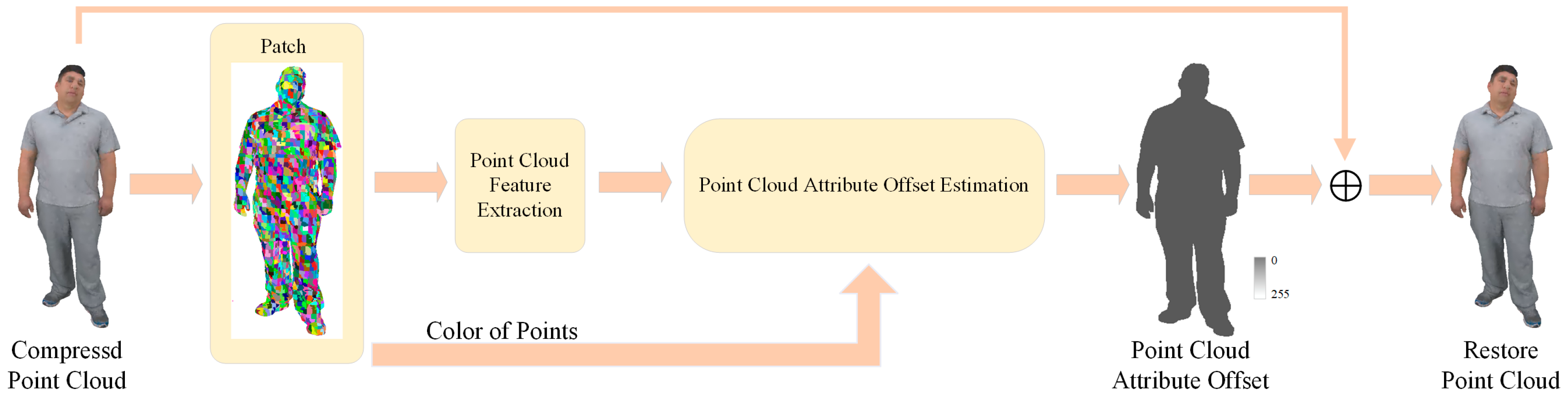
An iterative removal method for G-PCC attribute compression artifacts is proposed based on a GNN in this paper, aiming to improve the visual quality of compressed PCs, with the specific framework shown in Figure 2. In detail, to adapt to a large-scale PC and to ensure computational efficiency, this paper adopts a non-overlapping block segmentation strategy to divide the compressed PCs into multiple independent blocks of moderate size. During the feature extraction stage, a dynamic graph structure is introduced to construct a graph model that can capture the complex relationships between a point and its neighboring points, as well as between long-distance points. Given that different points may suffer from different degrees of information loss due to compression, the adaptive graph convolution is further implemented to automatically adjust the convolution kernel parameters according to the local features of the points, thus enhancing the attention to important artifact points. To maintain the spatial consistency of the PC attributes, a feature constraint mechanism is also designed, which extracts and integrates the global features as spatial constraints to ensure the coherence of PC attributes, while removing the artifacts. In addition, to compensate for the detail-related information that may be lost during the compression process, a bi-branch attention module is introduced to fuse the high-frequency features. By enhancing the ability to capture subtle features, it helps recover the detail-related features of PCs. Finally, an objective function is established within the attribute offset estimation module. The accurate estimation of attribute offsets is delivered by minimizing the squared distance between the model’s predicted sample offsets and the true offsets. To better estimate the attribute distortion in PCs, iteration is performed to estimate the additive offset of PC attributes. It is worth emphasizing that lossless compression is achieved regarding the geometric information, in other words, after compression and reconstruction, the coordinates of all the points in a PC remain unchanged, to avoid introducing geometric artifacts.
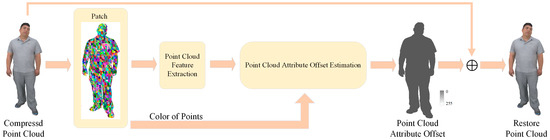
Figure 2.
Framework of the proposed method.
3.1. Point Cloud Chunking
For PCs with millions of points, it is not practical to directly input them into the neural network at one time, due to the physical constraint of the GPU memory capacity. To address this challenge, a chunking strategy is deployed. Specifically, a PC containing N points will be divided into many chunks, each of which has a fixed number (n) of points. Given that N is usually not divisible by n, a point-filling technique is further implemented, i.e., to add a certain number na (na < n) of filler points in the last PC chunk, so as to ensure that all the chunks reach the preset number (n) of points. It is worth noting that both the geometrical and attribute information of these filler points is replicated from the last valid point. In the subsequent processing and recovery phases, the filler points are removed to ensure that the PC chunks processed with the neural network can be accurately restored to their original state, thus excluding the potential interference introduced by the filler points. Through the implementation of chunking, massive PC data that are difficult to directly process can be successfully transformed into a series of smaller-scale and easy-to-process data chunks, thus enabling neural networks to process these massive datasets in an efficient, chunk-by-chunk manner, and significantly enhancing the processing efficiency and feasibility.
3.2. Feature Extraction Module
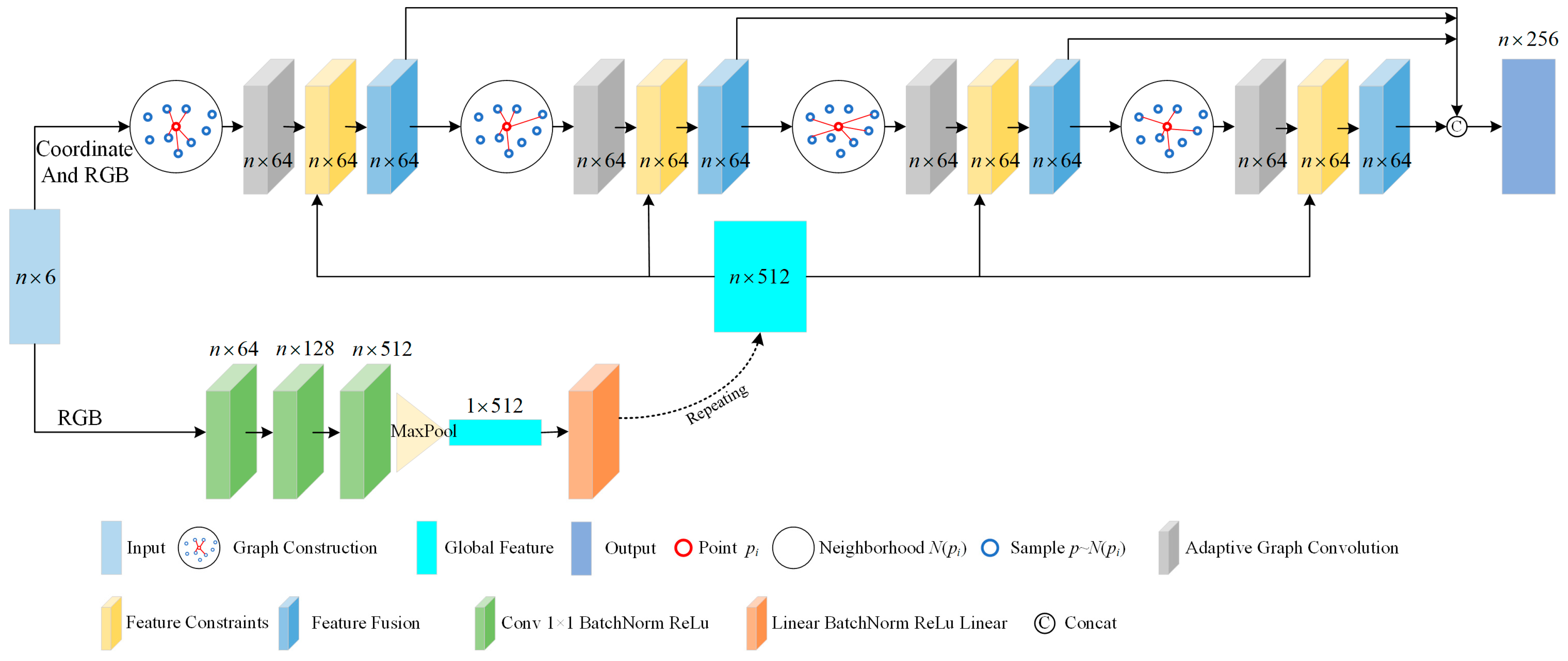
The feature extraction module covers dynamic graph structure modeling, adaptive graph convolution, feature constraints, and bi-branch attention. Specifically, to focus on global and local contexts, the module dynamically captures the complex short- and long-range correlations between a current point and its neighboring and distant points by means of the dynamic graph structure. Subsequently, adaptive graph convolution is introduced to focus on the points with a higher degree of artifacts, to extract and enhance their attribute features. Moreover, a feature constraint mechanism and a bi-branch attention mechanism are designed. The former is to maintain the spatial consistency of neighboring points at the attribute feature level during the PC recovery process, while the latter is to merge the high-frequency information and contextual information to effectively restore the fine features and texture details. Figure 3 intuitively showcases the architecture of the entire feature extraction module.
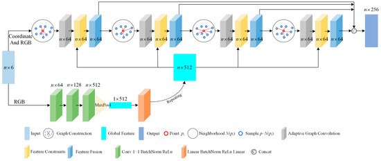
Figure 3.
The architecture of the entire feature extraction module.
Dynamic graph construction. For a given compressed PC P = {G,A}, where represents its geometric coordinate information and represents its color attribute. Here, i denotes the index of the points in a PC and N is the number of points. First, a directed self-loop graph = (,E) is constructed based on the coordinates of P to capture its intrinsic spatial structure, where = {vi|i = 1, …, N} represents the node set, which accurately maps each point in P, and E ⊆ × defines the edge set, which obtains the connectivity relationships among the nodes based on a specific proximity criterion (e.g., K-nearest neighbor algorithm), so as to ensure that each node vi ∈ is connected to its K nearest neighbors, including itself. Subsequently, to enhance the information representation of the graph, the edge eigenvectors are defined, where j denotes the index of neighboring points in the neighborhood of i-th center point, j = 1, 2, …, K, and, in particular, when j = 1, it denotes the connection of a node to itself. Specifically, any eij integrates the geometric coordinates Gi and the color attributes Ai of node vi, as well as the relative geometric features Gj-Gi and color features Aj − Ai between that node and its j-th neighboring point. In the above formula, dis(·) denotes the Euclidean distance metric function, which reflects the spatial proximity between the nodes and in turn enhances the differentiation of the features. It is worth noting that when j = 1, G1 and A1 are set to be the information of the node itself, ensuring that the self-connecting edges carry the complete information of the node, thus avoiding the loss of information, while maintaining the integrity of the graph structure. The concatenation operation [·,·] effectively merges spatial location and color attribute features into a unified eigenvector, capturing comprehensive node information.
Subsequently, a dynamic graph structure updating strategy based on feature similarity is used in the graph construction process, discarding the traditional method that relies on fixed spatial locations. Specifically, node similarity is evaluated in the feature dimension, allowing nodes with similar features to be grouped together, which dynamically reshapes the graph topology. This strategy enables the graph structure to capture intrinsic connections between a current point in the PC and distant points that share closely related features.
Overall, the dynamic graph construction strategy significantly broadens the receptive field of individual nodes within the network, while also enriching the feature input space for subsequent dynamic graph convolution operations. This mechanism enhances the network’s ability to capture and utilize both local and global dependencies, resulting in more accurate and insightful feature representations.
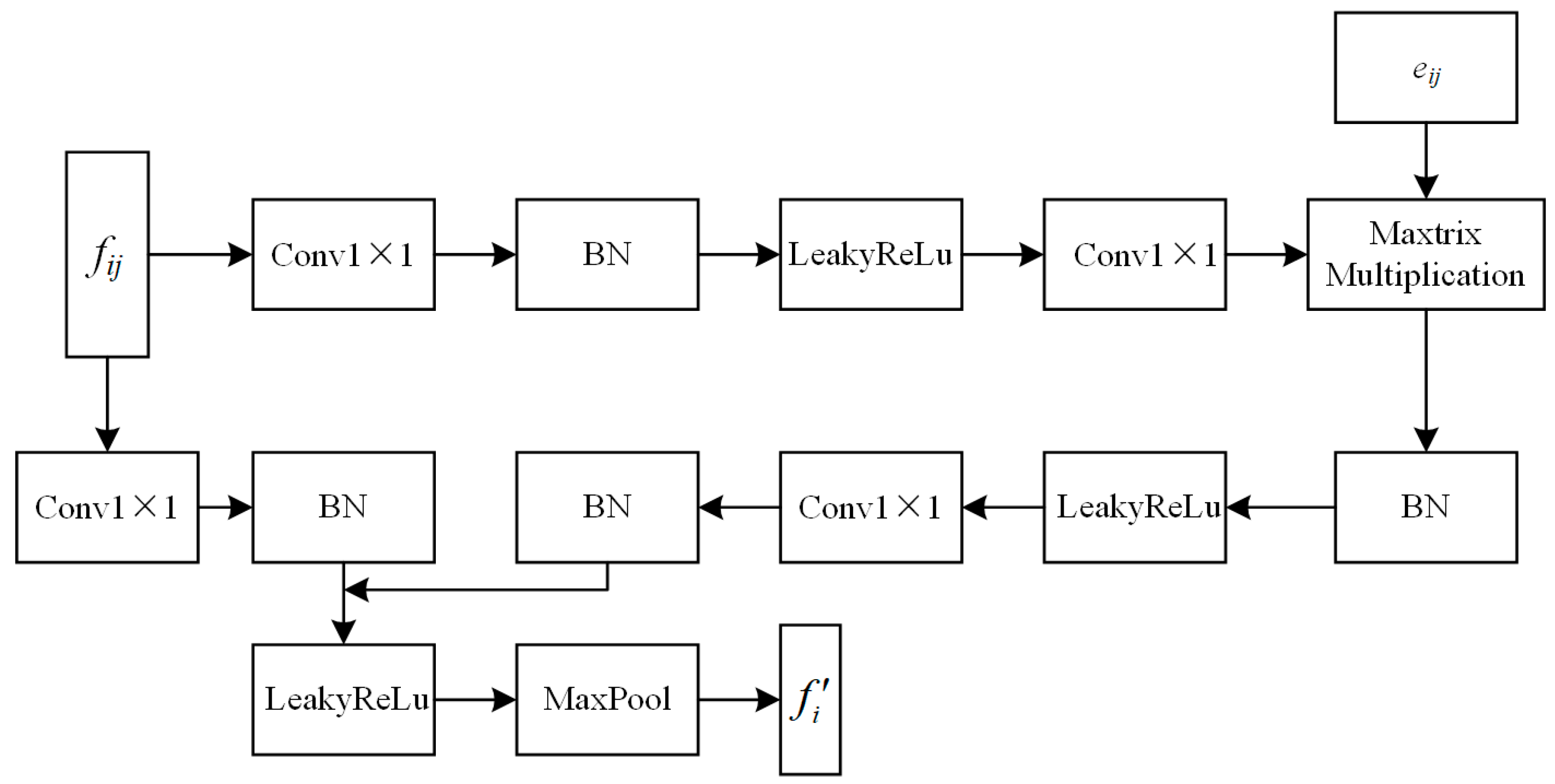
Adaptive graph convolution. To focus further on the points with a high amount of artifacts, adaptive graph convolution is introduced for feature extraction, with its structure shown in Figure 4. Specifically, an adaptive kernel is designed to capture the complex and unique geometric and contextual relationships in PCs. For each channel in terms of the M-dimensional output features, adaptive graph convolution dynamically generates the kernel using the point features:
where m = 1, 2, …, M denotes one of the output dimensions corresponding to a single filter defined in adaptive graph convolution and N(i) is the set of neighborhood points associated with node vi. To combine the global and local features, we define the edge feature eij as the input feature fij for the first adaptive kernel layer. Moreover, g(·) is a feature mapping function, consisting of a 1 × 1 convolutional layer, a BatchNorm layer, and a LeakyReLu activation layer.
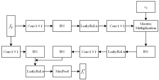
Figure 4.
The structure of adaptive graph convolution.
Similar to 2D convolution, the M output dimension is obtained by computing the convolution of the input features with the corresponding filter weights, i.e., the convolution of the adaptive kernel with the corresponding edges:
where denotes the inner product of two vectors outputting ∈ and σ(·) denotes the nonlinear activation function. The stacking of each channel generates the edge feature Sij = [, , …, ] ∈ between the connection points. Finally, the output feature of the central point vi is defined by applying the aggregation to all the edge features in the neighborhood.
where max(·) denotes the maximum pooling function and ⊕ represents an element-wise addition.
Additionally, fast and robust aggregation of the output features can be delivered by introducing a residual connection mechanism.
In general, the dynamic graph convolution achieves fine-grained extraction and characterization of PC data attributes. The core advantage lies in its ability to pay significant attention to and enhance the processing of distortion-significant regions in PC data, enabling the network model to more acutely identify and focus on these potentially challenging regions. In addition, it also facilitates the design and implementation of a feature constraint mechanism, making the feature regulation process more flexible and efficient.
Feature constraint mechanism. After compression, the attribute information of neighboring points in a PC should theoretically be spatially consistent, so as to ensure the visual effect of content rendering. Global features can capture the overall statistical information and structure of a PC, so that the neural network can deeply understand the attribute distribution and geometry. So, it is confirmed that global features can play a key role in the artifact removal process, guiding the network to adjust and optimize the extracted graph features at the macro level, thus improving the overall recovery effect. Therefore, a global feature-based constraint mechanism is designed and implemented to ensure that the recovery process strictly follows the principle of spatial consistency.
The core of the feature constraint mechanism designed as mentioned above consists in the scaling adjustment to the graph features of PCs. Specifically, its expression is:
where α denotes the global eigenvector of P and GFC(·) is the feature constraint function, which adjusts the graph feature according to α.
This process not only strengthens the correlation between the graph features and the global context, but also effectively promotes the maintenance of spatial consistency in the restoration process, resulting in a more visually coherent and natural PC.
By implementing the feature constraint mechanism, it can effectively mitigate abrupt changes during the recovery process, ensuring the continuity and smoothness of PC attribute information.
Bi-branch Attention Module. To address the problem that high-frequency information may get lost during the compression process, a bi-branch attention module is proposed, as shown in Figure 5. It is designed to deeply integrate the high-frequency features of PCs to accurately recover detailed information and improve the overall quality. In the bi-branch attention module, input features F are processed in parallel. One branch uses CNNs to directly represent feature mapping and transformations, in order to capture the basic structural information. Another branch performs high-frequency feature extraction, dedicated to mining and enhancing the high-frequency information in PCs. Specifically, the branch for high-frequency feature extraction first selects the significant maxima from the input features through a max-pooling operation, thus initially retaining the key texture information. Subsequently, this branch deeply processes the selected features through four consecutive unit layers (the first three unit layers consist of a 1 × 1 convolutional layer, a BatchNorm layer, and an ReLu layer, while the last omits the ReLu layer, to maintain feature flexibility) and then extracts the feature FH, which is rich in high-frequency details. Meanwhile, another branch applies the same sequence of the four unit layers directly to the input feature F to acquire a more general and optimized feature representation. Then, the output features from the two branches are preliminarily fused by element-by-element summation and further normalized in a Softmax layer to adjust the weights of each feature element, in order to ensure the rationality and effectiveness of the fusion process. Finally, the normalized result is multiplied with the input feature F in an element-by-element manner, in order to enhance the contribution of the high-frequency features in terms of the overall features and deliver the seamless fusion of the high-frequency features with the base features.
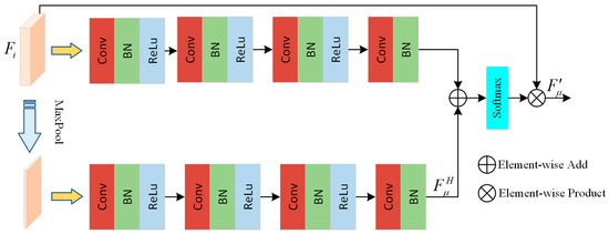
Figure 5.
The structure of the bi-branch attention module.
The expression for this process can be demonstrated as:
where Unit(·) denotes the processing function for the unit layer sequence, ⊙ denotes the element-by-element multiplication, and S(·) denotes the Softmax normalization function.
By introducing the innovative bi-branch attention module, it enables the deep extraction and efficient utilization of high-frequency features in PCs. This module not only compensates for the loss of high-frequency information during compression, but also enhances the complementarity and fusion between low- and high-frequency features. As a result, the recovered PC can accurately reproduce the detailed features of the original data, while preserving global structural integrity.
Layered feature concatenation. To address the problem of gradient vanishing or gradient explosion that may be encountered during the neural network backpropagation process, we adopt the strategy of layered feature concatenation. This strategy directs the output features of each bi-branch attention block to the terminal of the feature extraction architecture and integrates these features through the concatenation operation to form the final output feature , which is expressed as:
where concat(·) denotes the feature concatenation operation and denote the output features from the first to the fourth bi-branch attention blocks, respectively.
Such a layered feature concatenation strategy not only effectively maintains the fine-grained information independently extracted from each branch and avoids the loss of key information during the transmission process, but also captures the features more comprehensively by integrating multi-level feature representations.
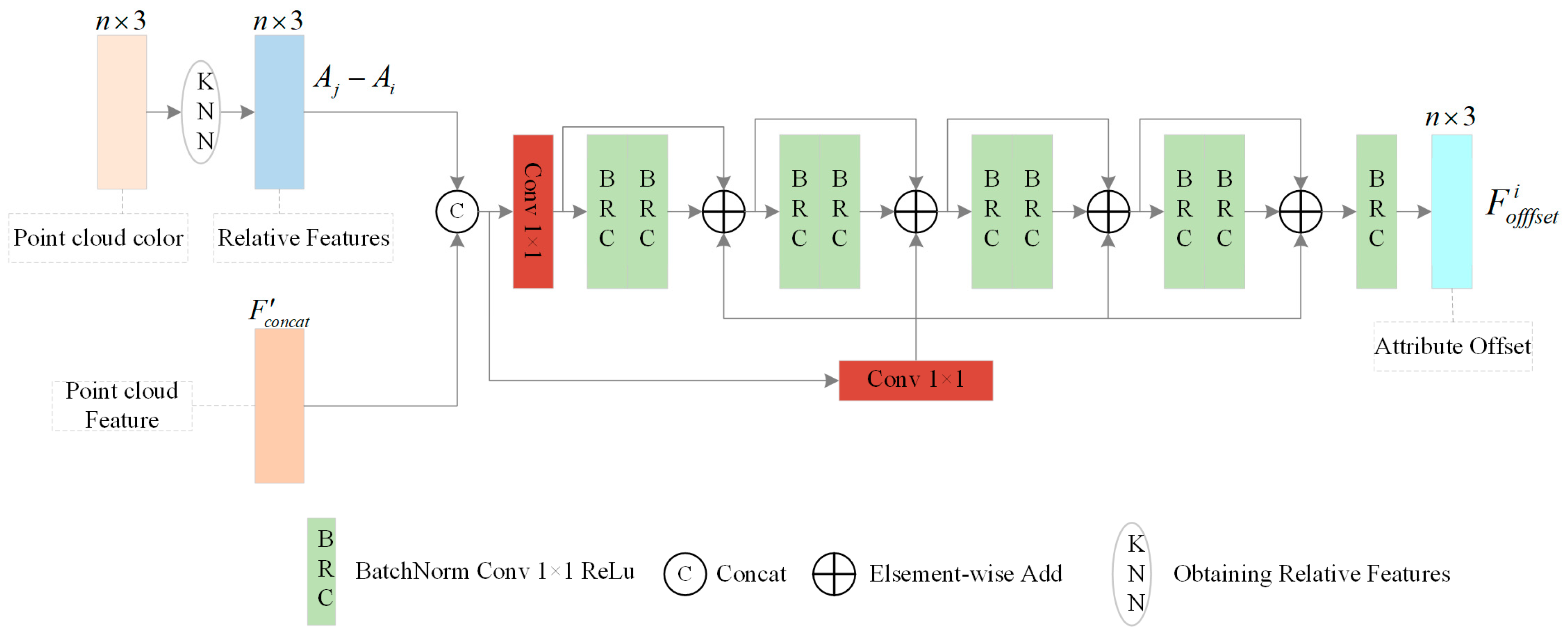
3.3. Point Cloud Attribute Offset Estimation Module
This module takes as the input parameter to estimate the offsets of the attributes. The structure is shown in Figure 6. Specifically, it takes an entire PC chunk as the input. Then, for any given 3D coordinates Gi, its K nearest neighbors are extracted as a sample set. Further, the attribute relative feature and are utilized to learn the PC attribute’s offset, denoted as Foffset. Formally, the module can be represented as:
where denotes the attribute offset of point Pi, Est(·) is a composite function consisting of a Multi-Layer Perceptron (MLP), and j ∈ N(i) are the neighboring points distributed in the attribute space of point Pi.
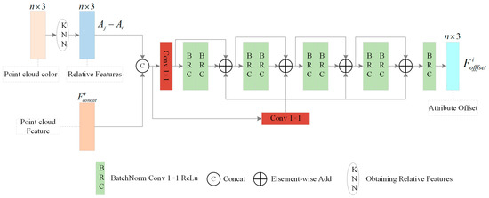
Figure 6.
The structure of the PC attribute offset estimation module.
Training objective. A training objective function is constructed, which aims to minimize the L2 norm squared distance between the predicted attribute offset and its true offsets. The original PC is defined as , which is used to compute the attribute offset of point Pi:
where is the difference vector in the attribute space between the original and compressed PCs, for this difference vector, can also be expressed as the displacement vector from the processed attribute state A to the original attribute state .
The training objective is to align the predictions of the module with the predefined offsets of the real attributes, so that the module can learn and predict the attribute offsets accurately:
where denotes the square of the L2 norm and E(·) denotes the expectation function; weighted averaging of the offset of the point properties occurs in the local neighborhood to reduce the overall error.
For a PC, the attribute information exhibits spatial consistency in space, i.e., neighboring points tend to have similar attribute characteristics, a phenomenon that does not exist in geometric coordinates. For this reason, we not only focus on the attribute offset prediction of point Pi at its own location, but also explore in-depth the attribute offset prediction in terms of its spatial neighborhood. This consideration aims to fully explore and utilize the rich attribute information within the local neighborhood of point Pi, so as to enhance the accuracy and robustness of attribute prediction.
The final training objective is to aggregate the predicted offsets of the local attributes about each point Pi and compute their mean values using the following expression:
where mean(·) denotes the average of the local attribute offsets of all the points in a PC.
This training objective can effectively balance the local prediction bias and promote equal consideration of the prediction contributions among different points. Furthermore, it includes a strong emphasis on the spatial consistency of attributes between the recovered PCs and the original PCs. By minimizing the mean value of the predicted offsets, the network can learn and simulate the spatial variation patterns of the original attributes of PCs, thereby reducing the impact of texture artifacts during the recovery process.
3.4. Iterative Removal of Artifacts
To reduce artifacts and optimize the texture quality of PCs, the attribute offsets of each point are first calculated, and this process is further extended to the K-nearest neighbors of each point. By calculating the weighted average of the attribute offsets of the neighboring points, the attribute offset information of the local region where point Pi is located is considered comprehensively, so as to improve the accuracy of capturing the attribute changes:
where KNN(Pi) denotes the neighborhood points of Pi.
After the abovemetioned calculation has been performed, an iterative updating method is further used to gradually adjust and optimize the attribute information of each point. And the iterative process is shown as follows:
where λt denotes the step size of the t-th iteration and its design follows two main guidelines: (1) λt gradually decreases and approaches 0 with the increase in the iteration number to ensure the convergence and stability of the iterative algorithm. (2) The value of λ1 is in the range of less than 1, but cannot be too close to 0, as according to Equation (5), too small a step size may lead to such an overly conservative estimation of the attribute offsets that the differences in the attribute values between the compressed PC and the original PC may not be adequately revealed.
Therefore, after an appropriate number of iterations for processing the compressed PC, the attribute compression artifacts can be effectively removed, and a better recovered PC can finally be acquired.
By implementing a well-designed iterative strategy, we effectively correct the additive bias in PC properties. The core strength of this strategy lies in its ability to incrementally approximate and compensate for the complex distortions introduced by systematic factors during compression, thereby significantly enhancing the visual quality and fidelity of the recovered PC.
4. Experiments
In this section, a series of experiments are carried out to quantitatively and qualitatively evaluate the performance of the proposed method in removing the texture artifacts in compressed PCs. In addition, some ablation experiments are also conducted to verify the effectiveness of the feature constraint mechanism and the high-frequency feature fusion. These experiments are conducive to comprehensively evaluating the robustness and performance of the proposed method.
4.1. Experiment Setup
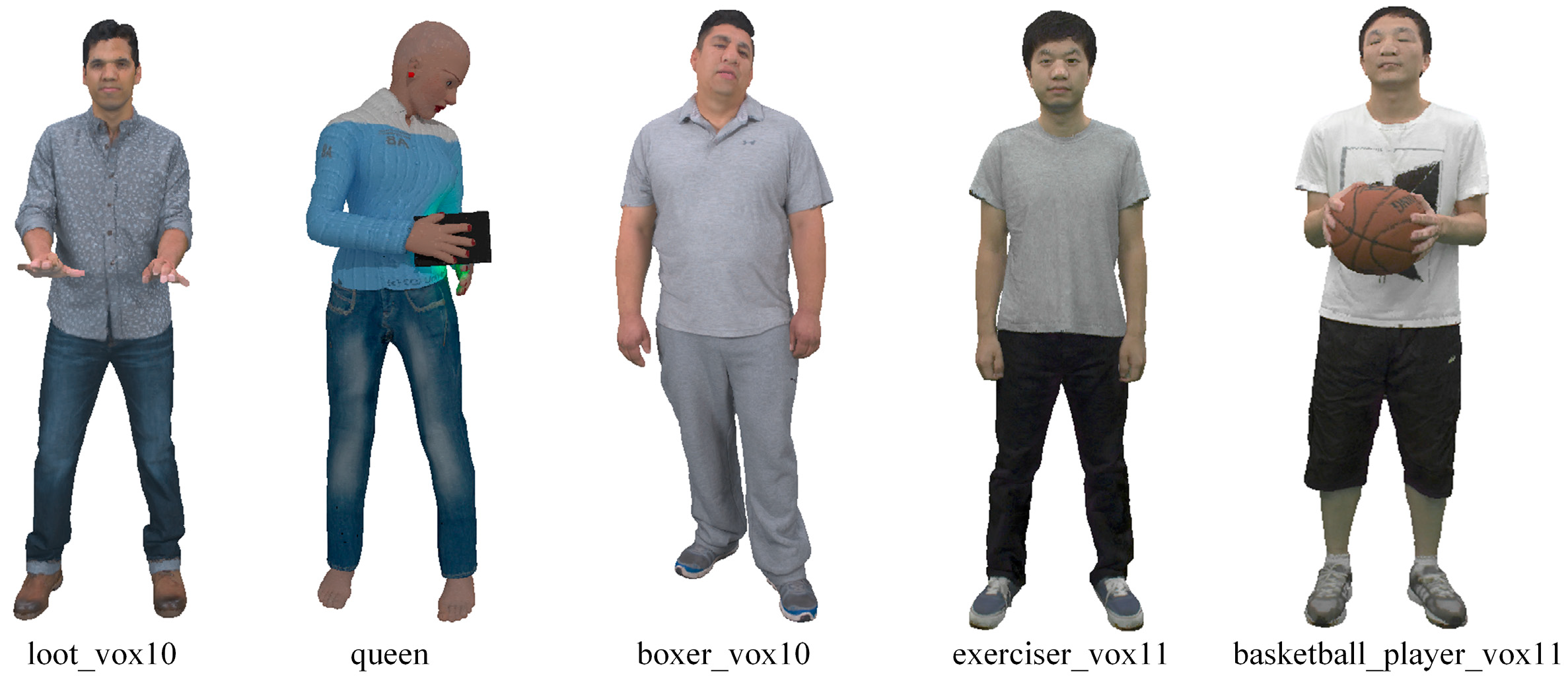
(1) Dataset. To train the proposed network model, we select five static PCs defined within the MPEG PC common test conditions [20,61,62], as original samples for generating a training set. The five static PCs are as follows, i.e., “basketball_player_vox11”, “loot_vox10”, “exerciser_vox11”, “queen”, and “boxer_vox10”, which present rich color and texture information, as shown in Figure 7. To generate the training samples, the latest G-PCC reference software TMC13v14 is used to compress these PCs, four differentiated attribute compression levels (i.e., R01, R02, R03, and R04) are set, and the default PredLift criterion is adopted to process the color attributes. It is worth noting that each attribute compression level trains a model independently.
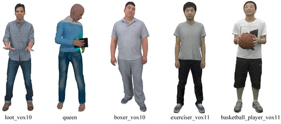
Figure 7.
Original PCs for generating the training dataset: “loot_vox10”, “queen”, “boxer_vox10”, “exerciser_vox11”, and “basketball_player_vox11” [20,61].
To validate the effectiveness of the proposed method, the same test samples provided by MS-GAT [56] are used in this paper. These samples include “Andrew”, “David”, “Phil”, “Ricardo”, “Sarah”, “Model”, “Longdress”, ”Red and black”, “Soldier”, and “Dancer”. It is worth noting that, unlike MS-GAT, the proposed method skips the step of transforming the RGB color space into the YUV color space during the processing, but directly uses the RGB attribute information as the input for the model. It simplifies the processing workflow and makes complete use of the color information in the PCs, without the need to train the three independent channels of Y, U, and V separately, thus improving the overall performance and efficiency of the model.
(2) Training and Testing Setup. We adopt NVIDIA GeForce RTX 3090 GPU (Nvidia, Santa Clara, CA, USA) for network model training. During the training process, the Adam optimization algorithm is used, for which the β1 and β2 parameters are set to 0.9 and 0.999, respectively, the learning rate is set to 10−4, and the batch size is set to 8. For the specific implementation, n, the point number in each patch, is set to 2048. In the feature extraction module, when the graph is constructed, K, the number of neighborhood points, is set to 16, and the dimension of the output feature for all layers is set to 64. For the artifact removal task, the iteration number is set to 2, aiming to effectively reduce the artifacts introduced during the compression process by a limited number of iterations and optimizations. Each network model is trained on the training dataset for 300 epochs.
(3) Performance Metrics. Two evaluation metrics are adopted to comprehensively and objectively measure the quality of the compressed PC after recovery. Firstly, since the color information in the PC is important for visual quality and the RGB peak signal-to-noise ratio (RGB-PSNR) is suitable for assessing the color fidelity of the compressed PC restoration task, we adopt the RGB-PSNR as the basic criterion for revealing the fidelity of PCs in terms of color, which can be calculated as follows:
where MAX is the maximum of the RGB color values and MSE is the mean square error between the recovered PC and the original PC in terms of the RGB color values.
Secondly, to better align with human visual perception, we also utilized the full-reference quality evaluation metric PCQM [63], which integrates both geometric and color information, offering high consistency in terms of subjective human perception. The smaller the PCQM [63] score, the better the quality of the PCs. It can be calculated as follows:
where ωG and ωA are the weights, the geometric feature fG is used to measure the difference in geometric structure between the two sets of PCs, and the color feature fA is used to measure the color difference between the original and recovered PCs.
4.2. Quantitative Quality Evaluation
To verify the performance of the proposed method in removing the attribute compression artifacts of PCs, it is compared with G-PCC [9] and MS-GAT [56]. For fairness, the data for training and testing are consistent across all methods. Table 2 presents the comparison results on the PredLift training and testing, and the optimal experimental results when compared to G-PCC are marked in bold, respectively. As found in Table 2, compared to G-PCC, the proposed method delivers good results for attribute recovery of the compressed PCs, with an average improvement of 3.40% for PCQM [63] and 0.34 dB for RGB-PSNR, indicating a significant quality improvement. As to the comparison with the MS-GAT [56] method, although it performs better for certain compressed PCs, there still exist some PCs with un-improved or even deteriorated quality. In contrast, the proposed method achieves positive quality gains on all the test samples, demonstrating its advantages in removing the attribute compression artifacts of PCs. Additionally, we have published the training curve of the network model, as shown in Figure 8. In the first 100 epochs, the training loss decreases relatively fast and eventually stabilizes with subsequent training rounds, indicating that the model exhibits good convergence using the dataset.
Table 2.
The objective quality metrics for attributes tested using the PredLift algorithm.
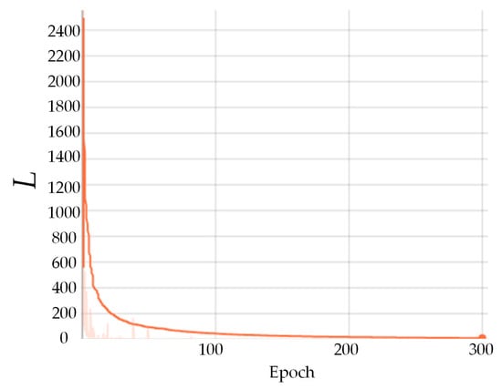
Figure 8.
Loss curve of a network model trained on a dataset for 300 epochs.
4.3. Qualitative Quality Evaluation
To demonstrate the performance of the proposed method in terms of the subjective visual quality, we visually present the recovered PCs, as shown in Figure 9. First, four samples compressed by G-PCC are showcased. As observed, the compressed PC illustrates obvious blurring and blocky features, especially the facial region in the human sample PC demonstrates obvious deformation and blurriness. For e.g., the face of “Phil” is severely blurred, while delivering remarkable blocky effects. After being optimized by the MS-GAT [56] method, the compressed PC is improved in terms of its visual quality, with a less blurred appearance generated. However, there is over-smoothing, which results in some details not being clearly rendered, for example, as seen in the faces of “Longdress”, “Phil”, and “Rachel”. In the case of “Longdress”, the facial details are not sufficiently restored, appearing to be excessively smooth and failing to effectively reproduce the fine structure of the original PC. This indicates that the MS-GAT [56] method is still yet to be optimized in terms of handling artifacts and retaining details.
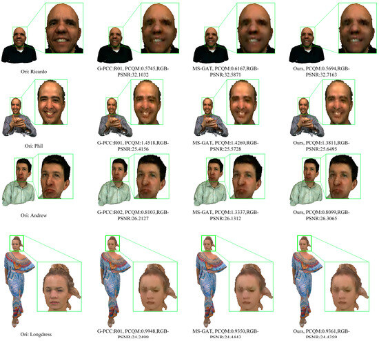
Figure 9.
Schematic diagram of the qualitative quality assessment results. Notes: ”ori” denotes the original PC [64]; “G-PCC” denotes the PC reconstructed using G-PCC TMC13v14; “MS-GAT” denotes the PC reconstructed using the MS-GAT [56] method; “Ours” denotes the PC reconstructed using the proposed method.
In contrast, the proposed method performs better in restoring the visual quality of the PCs. It can be found that, for the four samples, the proposed method delivers more natural restoration results, especially in the facial areas and in for some details, such as the nuances at the nose edge of “Ricardo”. These outcomes benefit mainly from the fact that the proposed method focuses on and incorporates high-frequency information. These visualization results further confirm the superiority of the proposed method. In particular, in recovering the detailed information of PCs, the proposed method showcases remarkable advantages and provides reliable visual evidence for the improvement of the PC quality.
4.4. Extended Application in Terms of RAHT
In order to further verify the generalization performance of the proposed method, a cross-configuration migration test is implemented. Specifically, the network model trained in regard to the G-PCC PredLift configuration is directly applied to the compressed PCs in the G-PCC RAHT configuration. The experimental results are shown in Table 3.
Table 3.
Quantitative comparison of the quality achieved with G-PCC on RAHT.
As clearly observed in Table 3, compared to G-PCC, the proposed method demonstrates a significant quality improvement in regard to the highest attribute compression level (i.e., R01). Specifically, the proposed method gains 0.07 dB in terms of the RGB-PSNR over G-PCC, while rendering a 0.67% gain in the PCQM [63] metric, thus further validating the effectiveness of the proposed method in boosting the quality of PCs. In particular, this performance improvement is delivered without any additional training for the specific configuration of G-PCC RAHT, therefore fully demonstrating the cross-configuration adaptability and generalizability of the proposed method.
4.5. Spatial, Temporal, and Computational Complexity
To quantitatively analyze the spatial and temporal complexity of the proposed method, the processing time for a compressed PC is calculated, and the spatial complexity is evaluated using the number of learnable parameters of a network model. A comparison between the MS-GAT [56] method and the proposed method is given and analyzed, and the results are shown in Table 4. For the MS-GAT [56] method, the following factors are comprehensively considered, i.e., block chunking for Y, U, and V components, thee block combination time, and the artifact removal time. It is worth noting that the processing time does not include the time for compressing and reading/writing files, to ensure a fair comparison. As can be found in Table 4, on average, the proposed method takes about 1/10 of the requirements needed by the MS-GAT method in terms of time for processing the compressed PCs, thus clearly illustrating the advantage of the proposed method in providing a processing speed that is 10-fold faster. In terms of the network model parameters, the scale of each separate color component in regard to the MS-GAT method is about 1.8 M, with a total of about 5.4 M learning parameters required. For the proposed method, the parameter scale of the whole network model is about 3.6M, meaning that 33% of the parameter space is saved. These results fully manifest the outstanding advantages of the proposed method in terms of performance and resource utilization. Moreover, to develop a more comprehensive performance evaluation framework, we additionally provide an analysis of the computational complexity of the network model. Given the MS-GAT [56] method does not cover the complete implementation code, our analysis of the computational complexity focuses on the elaboration of the self-methodology and is intended to provide a benchmark for subsequent studies. Specifically, as shown in Table 4, depending on the different sizes of the PCs, the required FLOPs for the proposed method range from 1.82 T to 21.19 T. Finally, we achieve an average of 7.65 T FLOPs.
Table 4.
Analysis and comparison of running time (in seconds) and computational complexity. The MS-GAT method and the proposed method are both run on the same GPU platform to process the compressed PCs. “Part” and “Comb” stand for the “Partition” and “Combination” of the block patch.
4.6. Ablation Experiments
The ablation experiments in this section are used to verify the effectiveness of the feature constraint mechanism and the bi-branch attention module, and further experimental analysis is conducted for the K number of neighboring points in the constructed graph.
The bi-branch attention block and the feature constraint mechanism. In this paper, the contribution of the bi-branch attention block and the feature constraint mechanism to the proposed method is investigated and the results are shown in Table 5. In this table, I denotes the baseline network model, which contains the complete implementation of all the modules, II represents the network without the bi-branch attention module, and III refers to the network without the feature constraint mechanism. By comparing models I and II, it can be observed that the baseline model outperforms the version without the bi-branch attention module. This result strongly demonstrates the key role of the bi-branch attention module in efficiently fusing the high-frequency features of PCs and also highlights its importance in accurately recovering fine texture details. The unique design of the bi-branch attention block effectively facilitates multi-level interaction and information enhancement, thereby improving the overall network’s ability to capture and recover intricate scene details. Furthermore, the comparison between models I and III demonstrates the positive impact of the feature constraint mechanism on the overall model performance. This mechanism significantly optimizes the quality of reconstructed PCs by enforcing spatial consistency during the recovery of PC attributes.
Table 5.
Analysis of the contribution of the feature constraint mechanism and the bi-branch attention module in the proposed method. The test is carried out on the G-PCC PredLift dataset at compression level R04.
The number (K) of the neighboring points in the constructed graph. To explore the optimal configuration for the number of neighboring points (K) used in graph construction, a series of ablation experiments are designed and implemented, with the results shown in Table 6. In this experiment, the values of K are set to 8, 12, 16, and 20, aiming to explore their effects on the removal of PC attribute compression artifacts. The results clearly showcase a significant statistical correlation between the value of K and the effectiveness of artifact removal. Overall, the performance of the proposed method shows a gradual enhancement trend with the gradual increase in the K value. This improvement can mainly be attributed to the fact that a larger K value can capture richer local neighborhood information, which helps to identify and remove attribute artifacts more accurately. However, when the K value is too large, feature redundancy may arise. While this increases the richness of the information, it also introduces a significant amount of weakly correlated or non-essential data. This can increase computational complexity, introduce noise, and reduce the model’s ability to discriminate between relevant features, ultimately degrading the overall performance. After considering all the factors and making careful analysis, we select the neighboring point number K = 16 as the optimal configuration. This selection strategy aims to achieve a delicate balance between maximizing the artifact removal effect and effectively controlling the computational overhead, achieving an optimal trade-off between efficiency and accuracy.
Table 6.
The effect on the network performance of the number (K) of neighboring points in the constructed graph. The test is carried out on the G-PCC PredLift dataset at compression level R04.
5. Conclusions
This paper develops an iterative removal method for attribute compression artifacts based on a graph neural network, with the aim of enhancing the visual quality of G-PCC compressed point clouds (PCs). It first takes the geometric coordinates of a compressed PC as the cornerstone for constructing the graph, while the attribute information is regarded as the vertex signals in the graph, so as to construct a graph that can reflect the properties of the PC. Given that different points may suffer from different degrees of artifacts during the compression process, adaptive graph convolution is introduced to dynamically adjust the parameters of the convolution kernel, thus extracting the attribute features in the severely damaged regions more effectively. Further, given that each point in the compressed PC may be correlated with its near- and far-distance points, a dynamic graph network structure is adopted to capture the correlation between a current point and its near- and far-distance points. Moreover, to ensure that the attribute information of neighboring points retains a certain level of spatial consistency, a feature constraint mechanism is designed. To address the problem of high-frequency information loss during the PC compression process, a bi-branch attention module is designed to fuse the high-frequency features of the compressed PC and effectively remedy the detail-recovery capability. The experimental results demonstrate that compared with the state-of-the-art methods, the proposed method has advantages in terms of improving the quality of G-PCC compressed PC attributes. The ablation experiments verified the key role of each module in the proposed method in boosting the overall performance.
Author Contributions
Data curation, L.L.; formal analysis, W.Y.; funding acquisition, Z.H.; methodology, Z.H.; supervision, R.B.; validation, W.Y. and L.L.; writing—original draft, W.Y.; writing—review and editing, Z.H. All authors have read and agreed to the published version of the manuscript.
Funding
This research was funded by the Natural Science Foundation of Zhejiang Province, grant number LQ23F010011, and Zhejiang Provincial Postdoctoral Research Excellence Foundation, grant number ZJ2022130.
Data Availability Statement
The original data presented in this study are openly available in [PCC Content Database] at [https://mpeg-pcc.org/index.php/pcc-content-database (accessed on 9 April 2023)], [PCC Datasets] at [http://mpegfs.int-evry.fr/MPEG/PCC/DataSets/pointCloud/CfP/datasets (accessed on 9 April 2023)], and [JPEG Pleno Database] at [https://plenodb.jpeg.org (accessed on 9 April 2023)].
Conflicts of Interest
Author Lijun Li was employed by the company Ningbo Cixing Co., Ltd. The remaining authors declare that the research was conducted in the absence of any commercial or financial relationships that could be construed as potential conflicts of interest.
References
- He, Y.; Li, B.; Ruan, J.; Yu, A.; Hou, B. ZUST Campus: A Lightweight and Practical LiDAR SLAM Dataset for Autonomous Driving Scenarios. Electronics 2024, 13, 1341. [Google Scholar] [CrossRef]
- Gamelin, G.; Chellali, A.; Cheikh, S.; Ricca, A.; Dumas, C.; Otmane, S. Point-cloud avatars to improve spatial communication in immersive collaborative virtual environments. Pers. Ubiquitous Comput. 2021, 25, 467–484. [Google Scholar] [CrossRef]
- Sun, X.; Song, S.; Miao, Z.; Tang, P.; Ai, L. LiDAR Point Clouds Semantic Segmentation in Autonomous Driving Based on Asymmetrical Convolution. Electronics 2023, 12, 4926. [Google Scholar] [CrossRef]
- Wang, Q.; Kim, M.K. Applications of 3D point cloud data in the construction industry: A fifteen-year review from 2004 to 2018. Adv. Eng. Inform. 2019, 39, 306–319. [Google Scholar] [CrossRef]
- Gao, P.; Zhang, L.; Lei, L.; Xiang, W. Point Cloud Compression Based on Joint Optimization of Graph Transform and Entropy Coding for Efficient Data Broadcasting. IEEE Trans. Broadcast. 2023, 69, 727–739. [Google Scholar] [CrossRef]
- Li, D.; Ma, K.; Wang, J.; Li, G. Hierarchical Prior-Based Super Resolution for Point Cloud Geometry Compression. IEEE Trans. Image Process. 2024, 33, 1965–1976. [Google Scholar] [CrossRef] [PubMed]
- Graziosi, D.; Nakagami, O.; Kuma, S.; Zaghetto, A.; Suzuki, T.; Tabatabai, A. An overview of ongoing point cloud compression standardization activities: Video-based (V-PCC) and geometry-based (G-PCC). APSIPA Trans. Signal Inf. Process. 2020, 9, e13. [Google Scholar] [CrossRef]
- MPEG 3DG. V-PCC Codec Description. In Document ISO/IEC JTC 1/SC 29/WG 11 MPEG, N19526; ISO/IEC: Newark, DE, USA, 2020.
- MPEG 3DG. G-PCC Codec Description. In Document ISO/IEC JTC 1/SC 29/WG 7 MPEG, N00271; ISO/IEC: Newark, DE, USA, 2020.
- Sullivan, G.J.; Ohm, J.R.; Han, W.J.; Wiegand, T. Overview of the high efficiency video coding (HEVC) standard. IEEE Trans. Circuits Syst. Video Technol. 2012, 22, 1649–1668. [Google Scholar] [CrossRef]
- Bross, B.; Chen, J.; Ohm, J.R.; Sullivan, G.J.; Wang, Y.K. Developments in international video coding standardization after AVC, with an overview of versatile video coding (VVC). Proc. IEEE 2021, 109, 1463–1493. [Google Scholar] [CrossRef]
- Huang, Y.; Peng, J.; Kuo, C.C.J.; Gopi, M. A generic scheme for progressive point cloud coding. IEEE Trans. Vis. Comput. Graph. 2008, 14, 440–453. [Google Scholar] [CrossRef]
- Jackins, C.L.; Steven, L.T. Oct-trees and their use in representing three-dimensional objects. Comput. Graph. Image Process. 1980, 14, 249–270. [Google Scholar] [CrossRef]
- Schnabel, R.; Reinhard, K. Octree-based Point-Cloud Compression. PBG@ SIGGRAPH 2006, 3, 111–121. [Google Scholar]
- Anis, A.; Chou, P.A.; Ortega, A. Compression of dynamic 3D point clouds using subdivisional meshes and graph wavelet transforms. In Proceedings of the 2016 IEEE International Conference on Acoustics, Speech and Signal Processing (ICASSP), Shanghai, China, 20–25 March 2016; pp. 6360–6364. [Google Scholar]
- Pavez, E.; Chou, P.A.; De Queiroz, R.L.; Ortega, A. Dynamic polygon clouds: Representation and compression for VR/AR. APSIPA Trans. Signal Inf. Process. 2018, 7, e15. [Google Scholar] [CrossRef]
- Mammou, K.; Tourapis, A.M.; Singer, D.; Su, Y. Video-based and hierarchical approaches point cloud compression. In Document ISO/IEC JTC1/SC29/WG11 m41649; ISO/IEC: Macau, China, 2017. [Google Scholar]
- Mammou, K.; Tourapis, A.; Kim, J.; Robinet, F.; Valentin, V.; Su, Y. Lifting scheme for lossy attribute encoding in TMC1. In Document ISO/IEC JTC1/SC29/WG11 m42640; ISO/IEC: San Diego, CA, USA, 2018. [Google Scholar]
- De Queiroz, R.L.; Chou, P.A. Compression of 3D point clouds using a region-adaptive hierarchical transform. IEEE Trans. Image Process. 2016, 25, 3947–3956. [Google Scholar] [CrossRef]
- PCC Content Database. Available online: https://mpeg-pcc.org/index.php/pcc-content-database (accessed on 9 April 2023).
- Karczewicz, M.; Hu, N.; Taquet, J.; Chen, C.-Y.; Misra, K.; Andersson, K.; Yin, P.; Lu, T.; François, E.; Chen, J. VVC in-loop filters. IEEE Trans. Circuits Syst. Video Technol. 2021, 31, 3907–3925. [Google Scholar] [CrossRef]
- Ma, D.; Zhang, F.; Bull, D.R. MFRNet: A new CNN architecture for post-processing and in-loop filtering. IEEE J. Sel. Top. Signal Process. 2020, 15, 378–387. [Google Scholar] [CrossRef]
- Nasiri, F.; Hamidouche, W.; Morin, L.; Dhollande, N.; Cocherel, G. A CNN-based prediction-aware quality enhancement framework for VVC. IEEE Open J. Signal Process. 2021, 2, 466–483. [Google Scholar] [CrossRef]
- Tsai, C.Y.; Chen, C.Y.; Yamakage, T.; Chong, I.S.; Huang, Y.-W.; Fu, C.-M.; Itoh, T.; Watanabe, T.; Chujoh, T.; Karczewicz, M.; et al. Adaptive loop filtering for video coding. IEEE J. Sel. Top. Signal Process. 2013, 7, 934–945. [Google Scholar] [CrossRef]
- Fu, C.M.; Alshina, E.; Alshin, A.; Huang, Y.W.; Chen, C.-Y.; Tsai, C.-Y.; Hsu, C.-W.; Lei, S.-M.; Park, J.-H.; Han, W.-J. Sample adaptive offset in the HEVC standard. IEEE Trans. Circuits Syst. Video Technol. 2012, 22, 1755–1764. [Google Scholar] [CrossRef]
- Norkin, A.; Bjontegaard, G.; Fuldseth, A.; Narroschke, M.; Ikeda, M.; Andersson, K.; Zhou, M.; Van der Auwera, G. HEVC deblocking filter. IEEE Trans. Circuits Syst. Video Technol. 2012, 22, 1746–1754. [Google Scholar] [CrossRef]
- Dong, C.; Deng, Y.; Loy, C.C.; Tang, X. Compression artifacts reduction by a deep convolutional network. In Proceedings of the IEEE International Conference on Computer Vision, Santiago, Chile, 7–13 December 2015; pp. 576–584. [Google Scholar]
- Wang, Z.; Ma, C.; Liao, R.L.; Ye, Y. Multi-density convolutional neural network for in-loop filter in video coding. In Proceedings of the 2021 Data Compression Conference (DCC), Snowbird, UT, USA, 23–26 March 2021; pp. 23–32. [Google Scholar]
- Lin, K.; Jia, C.; Zhang, X.; Wang, S.; Ma, S.; Gao, W. Nr-cnn: Nested-residual guided cnn in-loop filtering for video coding. ACM Trans. Multimed. Comput. Commun. Appl. (TOMM) 2022, 18, 1–22. [Google Scholar] [CrossRef]
- Pan, Z.; Yi, X.; Zhang, Y.; Jeon, B.; Kwong, S. Efficient in-loop filtering based on enhanced deep convolutional neural networks for HEVC. IEEE Trans. Image Process. 2020, 29, 5352–5366. [Google Scholar] [CrossRef] [PubMed]
- Jia, W.; Li, L.; Li, Z.; Zhang, X.; Liu, S. Residual-guided in-loop filter using convolution neural network. ACM Trans. Multimed. Comput. Commun. Appl. (TOMM) 2021, 17, 1–19. [Google Scholar] [CrossRef]
- Zhang, Y.; Shen, T.; Ji, X.; Zhang, Y.; Xiong, R.; Dai, Q. Residual highway convolutional neural networks for in-loop filtering in HEVC. IEEE Trans. Image Process. 2018, 27, 3827–3841. [Google Scholar] [CrossRef] [PubMed]
- Wang, D.; Xia, S.; Yang, W.; Liu, J. Combining progressive rethinking and collaborative learning: A deep framework for in-loop filtering. IEEE Trans. Image Process. 2021, 30, 4198–4211. [Google Scholar] [CrossRef]
- Kong, L.; Ding, D.; Liu, F.; Mukherjee, D.; Joshi, U.; Chen, Y. Guided CNN restoration with explicitly signaled linear combination. In Proceedings of the 2020 IEEE International Conference on Image Processing (ICIP), Abu Dhabi, United Arab Emirates, 25–28 October 2020; IEEE: Piscataway, NJ, USA, 2020; pp. 3379–3383. [Google Scholar]
- Quach, M.; Valenzise, G.; Dufaux, F. Folding-based compression of point cloud attributes. In Proceedings of the 2020 IEEE International Conference on Image Processing (ICIP), Abu Dhabi, United Arab Emirates, 25–28 October 2020; pp. 3309–3313. [Google Scholar]
- Wang, J.; Ding, D.; Li, Z.; Ma, Z. Multiscale point cloud geometry compression. In Proceedings of the 2021 Data Compression Conference (DCC), Snowbird, UT, USA, 23–26 March 2021; pp. 73–82. [Google Scholar]
- Guarda, A.F.; Rodrigues, N.M.; Pereira, F. Adaptive deep learning-based point cloud geometry coding. IEEE J. Sel. Top. Signal Process. 2020, 15, 415–430. [Google Scholar] [CrossRef]
- Quach, M.; Valenzise, G.; Dufaux, F. Learning convolutional transforms for lossy point cloud geometry compression. In Proceedings of the 2019 IEEE International Conference on Image Processing (ICIP), Taipei, Taiwan, 22–29 September 2019; pp. 4320–4324. [Google Scholar]
- Qi, C.R.; Su, H.; Mo, K.; Guibas, L.J. Pointnet: Deep learning on point sets for 3d classification and segmentation. In Proceedings of the IEEE Conference on Computer Vision and Pattern Recognition, Honolulu, HI, USA, 21–26 July 2017; pp. 652–660. [Google Scholar]
- Qi, C.R.; Yi, L.; Su, H.; Guibas, L.J. Pointnet++: Deep hierarchical feature learning on point sets in a metric space. Adv. Neural Inf. Process. Syst. 2017, 30, 2. [Google Scholar]
- Wang, Y.; Sun, Y.; Liu, Z.; Sarma, S.E.; Bronstein, M.M.; Solomon, J.M. Dynamic graph cnn for learning on point clouds. ACM Trans. Graph. (TOG) 2019, 38, 1–12. [Google Scholar] [CrossRef]
- Chen, C.; Fragonara, L.Z.; Tsourdos, A. GAPointNet: Graph attention based point neural network for exploiting local feature of point cloud. Neurocomputing 2021, 438, 122–132. [Google Scholar] [CrossRef]
- Wang, L.; Huang, Y.; Hou, Y.; Zhang, S.; Shan, J. Graph attention convolution for point cloud semantic segmentation. In Proceedings of the IEEE/CVF Conference on Computer Vision and pattern Recognition, Long Beach, CA, USA, 15–20 June 2019; pp. 10296–10305. [Google Scholar]
- Shi, W.; Rajkumar, R. Point-gnn: Graph neural network for 3d Object detection in a point cloud. In Proceedings of the IEEE/CVF Conference on Computer Vision and Pattern Recognition, Seattle, WA, USA, 13–19 June 2020; pp. 1711–1719. [Google Scholar]
- Te, G.; Hu, W.; Zheng, A.; Guo, Z. Rgcnn: Regularized graph cnn for point cloud segmentation. In Proceedings of the 26th ACM International Conference on Multimedia, Seoul, Republic of Korea, 22–26 October 2018; pp. 746–754. [Google Scholar]
- Chen, S.; Duan, C.; Yang, Y.; Li, D.; Feng, C.; Tian, D. Deep unsupervised learning of 3D point clouds via graph topology inference and filtering. IEEE Trans. Image Process. 2019, 29, 3183–3198. [Google Scholar] [CrossRef]
- Liang, Z.; Yang, M.; Deng, L.; Wang, C.; Wang, B. Hierarchical depthwise graph convolutional neural network for 3D semantic segmentation of point clouds. In Proceedings of the 2019 International Conference on Robotics and Automation (ICRA), Montreal, QC, Canada, 20–24 May 2019; pp. 8152–8158. [Google Scholar]
- Zhang, C.; Florencio, D.; Loop, C. Point cloud attribute compression with graph transform. In Proceedings of the 2014 IEEE International Conference on Image Processing (ICIP), Paris, France, 27–30 October 2014; pp. 2066–2070. [Google Scholar]
- Hammond, D.K.; Vandergheynst, P.; Gribonval, R. Wavelets on graphs via spectral graph theory. Appl. Comput. Harmon. Anal. 2011, 30, 129–150. [Google Scholar] [CrossRef]
- Haar, A. Zur Theorie der Orthogonalen Funktionensysteme; Georg-August-Universitat: Gottingen, Germany, 1909. [Google Scholar]
- Schwarz, S.; Preda, M.; Baroncini, V.; Budagavi, M.; Cesar, P.; Chou, P.A.; Cohen, R.A.; Krivokuća, M.; Lasserre, S.; Li, Z.; et al. Emerging MPEG standards for point cloud compression. IEEE J. Emerg. Sel. Top. Circuits Syst. 2018, 9, 133–148. [Google Scholar] [CrossRef]
- Sheng, X.; Li, L.; Liu, D.; Xiong, Z.; Li, Z.; Wu, F. Deep-PCAC: An end-to-end deep lossy compression framework for point cloud attributes. IEEE Trans. Multimed. 2021, 24, 2617–2632. [Google Scholar] [CrossRef]
- He, Y.; Ren, X.; Tang, D.; Zhang, Y.; Xue, X.; Fu, Y. Density-preserving deep point cloud compression. In Proceedings of the IEEE/CVF Conference on Computer Vision and Pattern Recognition, New Orleans, LA, USA, 18–24 June 2022; pp. 2333–2342. [Google Scholar]
- Wang, J.; Ma, Z. Sparse tensor-based point cloud attribute compression. In Proceedings of the 2022 IEEE 5th International Conference on Multimedia Information Processing and Retrieval (MIPR), Virtual, 2–4 August 2022; IEEE: Piscataway, NJ, USA; pp. 59–64. [Google Scholar]
- Fang, G.; Hu, Q.; Wang, H.; Xu, Y.; Guo, Y. 3dac: Learning attribute compression for point clouds. In Proceedings of the IEEE/CVF Conference on Computer Vision and Pattern Recognition, New Orleans, LA, USA, 18–24 June 2022; pp. 14819–14828. [Google Scholar]
- Sheng, X.; Li, L.; Liu, D.; Xiong, Z. Attribute artifacts removal for geometry-based point cloud compression. IEEE Trans. Image Process. 2022, 31, 3399–3413. [Google Scholar] [CrossRef]
- Ding, D.; Zhang, J.; Wang, J.; Ma, Z. CARNet: Compression Artifact Reduction for Point Cloud Attribute. arXiv 2022, arXiv:2209.08276. [Google Scholar]
- Xing, J.; Yuan, H.; Hamzaoui, R.; Liu, H.; Hou, J. GQE-Net: A graph-based quality enhancement network for point cloud color attribute. IEEE Trans. Image Process. 2023, 32, 6303–6317. [Google Scholar] [CrossRef]
- Zhang, K.; Hao, M.; Wang, J.; Chen, X.; Leng, Y.; de Silva, C.W.; Fu, C. Linked dynamic graph cnn: Learning through point cloud by linking hierarchical features. In Proceedings of the 2021 27th International Conference on Mechatronics and Machine Vision in Practice (M2VIP), Shanghai, China, 26–28 November 2021; pp. 7–12. [Google Scholar]
- Wei, M.; Wei, Z.; Zhou, H.; Hu, F.; Si, H.; Chen, Z.; Zhu, Z.; Qiu, J.; Yan, X.; Guo, Y.; et al. AGConv: Adaptive graph convolution on 3D point clouds. IEEE Trans. Pattern Anal. Mach. Intell. 2023, 45, 9374–9392. [Google Scholar] [CrossRef]
- PCC DataSets. Available online: http://mpegfs.int-evry.fr/MPEG/PCC/DataSets/pointCloud/CfP/datasets (accessed on 9 April 2023).
- Schwarz, S.; Martin, C.G.; Flynn, D.; Budagavi, M. Common test conditions for point cloud compression. In Document ISO/IEC JTC1/SC29/WG11 w17766; Ljubljana, Slovenia, 2018.
- Meynet, G.; Nehmé, Y.; Digne, J.; Lavoué, G. PCQM: A full-reference quality metric for colored 3D point clouds. In Proceedings of the 2020 Twelfth International Conference on Quality of Multimedia Experience (QoMEX), Virtual, 26–28 May 2020; pp. 1–6. [Google Scholar]
- JPEG Pleno Database. Available online: https://plenodb.jpeg.org (accessed on 9 April 2023).


Disclaimer/Publisher’s Note: The statements, opinions and data contained in all publications are solely those of the individual author(s) and contributor(s) and not of MDPI and/or the editor(s). MDPI and/or the editor(s) disclaim responsibility for any injury to people or property resulting from any ideas, methods, instructions or products referred to in the content. |
© 2024 by the authors. Licensee MDPI, Basel, Switzerland. This article is an open access article distributed under the terms and conditions of the Creative Commons Attribution (CC BY) license (https://creativecommons.org/licenses/by/4.0/).