Article

Stability of Local Trajectory Planning for Level-2+ Semi-Autonomous Driving without Absolute Localization

1
Automated Driving Lab, The Ohio State University, Columbus, OH 43212, USA
2
State Key Laboratory of Automotive Simulation and Control, Jilin University, Changchun 130022, China
*
Author to whom correspondence should be addressed.
Electronics 2024, 13(19), 3808; https://doi.org/10.3390/electronics13193808
Submission received: 28 August 2024 / Revised: 23 September 2024 / Accepted: 24 September 2024 / Published: 26 September 2024
(This article belongs to the Special Issue Intelligent Technologies for Vehicular Networks, 2nd Edition)

Abstract

:
Autonomous driving has long grappled with the need for precise absolute localization, making full autonomy elusive and raising the capital entry barriers for startups. This study delves into the feasibility of local trajectory planning for Level-2+ (L2+) semi-autonomous vehicles without the dependence on accurate absolute localization. Instead, emphasis is placed on estimating the pose change between consecutive planning timesteps from motion sensors and on integrating the relative locations of traffic objects into the local planning problem within the ego vehicle’s local coordinate system, thereby eliminating the need for absolute localization. Without the availability of absolute localization for correction, the measurement errors of speed and yaw rate greatly affect the estimation accuracy of the relative pose change between timesteps. This paper proved that the stability of the continuous planning problem under such motion sensor errors can be guaranteed at certain defined conditions. This was achieved by formulating it as a Lyapunov-stability analysis problem. Moreover, a simulation pipeline was developed to further validate the proposed local planning method, which features adjustable driving environment with multiple lanes and dynamic traffic objects to replicate real-world conditions. Simulations were conducted at two traffic scenes with different sensor error settings for speed and yaw rate measurements. The results substantiate the proposed framework’s functionality even under relatively inferior sensor errors distributions, i.e., speed error v err N ( 0.1 , 0.1 ) m/s and yaw rate error θ ˙ err N ( 0.57 , 1.72 ) deg/s. Experiments were also conducted to evaluate the stability limits of the planned results under abnormally larger motion sensor errors. The results provide a good match to the previous theoretical analysis. Our findings suggested that precise absolute localization may not be the sole path to achieving reliable trajectory planning, eliminating the necessity for high-accuracy dual-antenna Global Positioning System (GPS) as well as the pre-built high-fidelity (HD) maps for map-based localization.

1. Introduction

1.1. Background

Over the years, fully autonomous driving has struggled to achieve reliability and large-scale implementation. Even today, leading representatives in autonomous driving, such as Waymo and Cruise, face challenges navigating urban environments like San Francisco, with their driverless vehicles occasionally clogging traffic in the middle of the road [1,2]. Despite more than a decade of industry R&D, driverless autonomous solutions appear far from successful business applications based on current performance. Meanwhile, autonomous driving startups are rapidly consuming investments. Uber alone reportedly spent an annual $457 million on self-driving R&D before selling its unit to Aurora [3]. Over time, investors have become less attracted to driverless technology and increasingly hesitant about the technology’s potential business yields in the near future. The landmark shutdown of the star unicorn startup Argo AI [4] and the closure of the first public self-driving truck company Embark Technology [5] both reflect the struggles of Level-4 (L4) startups to secure capital funding. The heightened global economic uncertainty, along with potential recession, exacerbates this struggle. L4 providers like Waymo and TuSimple have reportedly laid off large numbers of employees to cut operating costs [6,7].
The valuation of autonomous driving startups has plummeted drastically in recent times. Waymo’s valuation dropped 80% from $200 billion to $30 billion in just 18 months. TuSimple’s stock, which once peaked above $60, now stands at slightly above $1 as of April 2023. In contrast, Tesla’s Autopilot driver assistance system, first deployed in 2014, has been a significant feature that greatly promotes the sale of Tesla vehicles. Its so-called Full Self-Driving (FSD) add-on package, though questionably named, directly contributed $324 million in revenue for the fourth quarter alone in 2022 [8]. The FSD package is so popular that 19% of Tesla owners opted in despite the price hike from an initial $5000 in 2019 to $15,000 in 2022 [9]. The debate over the autonomous driving development strategy between Tesla and Waymo has persisted for years [10]. Tesla insisted on a progressive evolution path with a vision-based solution that emphasizes cost reduction and mass production application, while Waymo aimed for an all-in-one driverless solution from day one, incorporating advanced and expensive sensors like LiDAR and relying heavily on detailed prerequisite information, such as high-definition (HD) maps. As of now, it seems that the Tesla approach prevails in the industry, generating continuous cash flow to back support its own progression.
The classification of autonomous driving from levels 0 to 5, as defined by the SAE [11], ranges from full human control (Level-0) to complete automation without any human intervention (Level-5). Level-4, which is closest to full autonomy, operates within a predefined operational design domain (ODD) and does not guarantee autonomous operation outside these boundaries, such as beyond a geofenced area or in severe snow conditions. Currently, production vehicles equipped with Advanced Driver Assistance Systems (ADAS) already reach Level-2 (L2), offering partial automation features like adaptive cruise control (ACC) and lane keeping assist (LKA) under limited driving conditions. The enhanced L2+ ADAS further expands the operational scope of L2, enabling complex tasks like lane changes and handling intersection scenarios in both urban and highway settings through features such as Navigate on Autopilot (NOA).
The autonomous vehicle industry has quietly but largely shifted interest towards the cost-efficient L2+ semi-autonomous driving solutions. Semi-autonomous driving, ranging from L2 to L3, still requires close human supervision and timely intervention, which is distinct from fully autonomous driving solutions operating without the need for human intervention. OEMs are especially interested in the potential highway and urban NOA feature [12], an L2+ feature that traditional Level-1 suppliers are unable to provide, to assist driver navigate in complex urban scenarios. L2+ solutions do not guarantee driving safety and demand human attention and intervention during driving. In such applications, “The driver is still responsible for, and ultimately in control of, the car”, as Tesla stated [13]. This easing of liability and the compromise on fully self-driving realization provide L4 startups a midway transition to package their solutions into a viable product. However, this transition is not merely a hardware downgrade and algorithm transplant. The lite version of hardware may imply fewer available resources, such as weaker computing power, the unavailability of sensor data, or less accurate measurement data, among others. As a result, transplanting L4 algorithms, which are designed for data-abundant hardware platforms, to fit L2+ applications is not as simple as it may seem [14].

1.2. Related Work

The centimeter-level accuracy of absolute localization is essential for L4 driving, which relies on detailed lane information available in HD maps. Several mature localization techniques exist in the L4 driving system to achieve this high precision. The Global Navigation Satellite Systems (GNSS)-based method, such as dual-antenna GPS enhanced by real-time kinematic (RTK) systems, is the most straight-forward and widely adopted solution for L4 vehicles [15,16]. The GNSS-based method, however, suffers from performance degradation in urban areas with satellite signal obstructions [17]. The high-precision solution such as RTK-GPS products are also prohibitively expensive. An alternative approach is map-based localization, wherein sensors such as LiDAR or camera continuously scan the environment and match the collected data against a pre-built HD map to localize the vehicle with high accuracy [18,19]. This technique gained popularity in L4 systems, as HD maps provide rich details such as lane markings and traffic signs, thereby reducing the burden on its perception system. However, the pre-built HD maps require continuous updates to align with the ever-changing road environment. The lack of the map’s widespread coverage also limits the adoption of the map localization method. The SLAM technique, originally introduced in robotics [20], is well-suited for low-speed unstructured driving environments like parking garages [21,22]. SLAM allows the vehicle to construct and update its own map in real time as it moves through the environment. However, SLAM is computationally intensive and requires substantial memory to store the constructed maps, making it less practical for high-speed or large-scale environments [23,24]. In L4 driving, these localization methods are often used in combination, leveraging the strengths of each method through sensor fusion to achieve the necessary accuracy and robustness.
However, in cost-sensitive mass production, L2+ vehicles may not come equipped with an expensive dual-antenna GPS or LiDAR sensor. HD maps are also not available to cover every traffic route to work with map-based localization. Therefore, in L2+ applications, the centimeter-level accuracy of absolute localization is not available, making it one of the key challenges for semi-autonomous driving. Now the following question arises: without this critical absolute localization information, is semi-autonomous driving still technically feasible?
Consider the following case of human driving: human drivers do not necessarily need to be aware of their absolute localization in terms of centimeter-level accuracy. Humans also do not have the detailed lane-to-lane transition routes at an intersection beforehand, as HD maps provide. They are more aware of the surroundings, such as the distance from other traffic objects or whether they are in the correct lane. This analogy to human driving may seem simplistic, but it implies that L2+ semi-autonomous driving may be feasible without accurate absolute localization, by instead using relative localization. Relative localization refers to the process of determining the relative position and orientation of the ego vehicle with respect to the surrounding environment, including other vehicles, pedestrians, and obstacles. The relative localization is typically achieved from perception system using a combination of sensors such as cameras, radars, and possibly LiDARs, which are available for L2+ ready vehicles.
But how does the local trajectory planning work with relative localization? During planning, one consideration is the trajectory consistency, meaning the trajectories planned in consecutive timesteps must maintain or approximate the spatial and temporal continuity. This is achievable for absolute localization, since the ego vehicle localization, planned trajectories, and traffic object movements are all under the same global coordinate system. However, for relative localization, there is no way to accurately reflect all these information under the global coordinate system. Few research studies have been addressed this practical problem. To ensure the consistency of the planned trajectory, we emphasized that relative localization with respect to surrounding traffic between adjacent timesteps must be taken into account. The relative motion of the ego vehicle between adjacent timesteps can be estimated by the existing odometry method, including inertial measurement unit (IMU)-based and visual odometry methods. The IMU-based odometry integrates acceleration and yaw rate data from the IMU sensor to estimate motion [25]. The visual odometry technique uses images from onboard cameras to track feature points in the environment and estimate the vehicle’s movements by analyzing the relative changes of these feature points [26]. Both methods will inevitably introduce errors in the estimation of position and posture changes. The inertial navigation system (INS) is based on exactly this idea to estimate absolute localization, but it needs periodic correction/fusion with GNSS data to avoid the build-up of the integration errors. In the L2+ semi-autonomous driving case, there is no accurate source to correct the estimate of absolute localization. Therefore, instead of choosing global coordinates, trajectory planning for L2+ semi-autonomous driving was carried out under the local vehicle coordinates. The trajectory from last timestep was projected to the local vehicle coordinate at the current timestep to ensure planning consistency. In this way, the localization error is limited between timesteps and will not accumulate.
Although the trajectory planning topic is not new in research fields with different approaches based on spline [27,28], potential fields [29], a sampling method [30,31], a graph search [32], optimization [33], and so on, few have evaluated the dynamic stability of the continuously changing planned trajectories. Trajectory planning is usually continuously ongoing in cycles and may be subject to change in response to perturbations, including changes in the environment, sensor noise, execution errors from control, and model uncertainties from vehicle dynamics and the environment. It is important to ensure the planned trajectory is stable and feasible under such perturbations. Ref. [34] presented a learning-based motion planning with stability guaranteed by designing a differential Lyapunov function using contraction theory. In [35], a motion planning framework was designed to maximize a marine vehicle’s stability margins against ocean disturbances. However, few comparable analysis have been seen for trajectory planning in autonomous driving field. Ref. [36] demonstrated the stability of the cost-based lattice controller in event of dynamic environment change but limited to simulation without rigorous theoretical proof. Under the context of trajectory planning without absolute localization, the drift and offset errors from the IMU sensor could build up the estimated relative localization error and affect the continuously planning stability. Hence, this paper specifically considers perturbations from relative localization and proves the necessary conditions under which the trajectory planning could maintain dynamic stability.

1.3. Present Contribution

One major contribution from this paper is the proposal of a local trajectory planning framework that works without the availability of absolute localization, which is challenging for L2+ semi-autonomous driving applications with limited hardware. Another contribution comes from the proof and conclusion that the stability of the dynamic trajectory planning subject to motion-sensor errors could be ensured under certain easy-to-meet conditions. The stability of the proposed local trajectory planning framework is also further validated under different simulation scenarios given the drifting and offset noise from the IMU sensor. This paper could provide some insights and prove the validity for an L2+ semi-autonomous application development with limited hardware equipment.
The structure of this paper is as follows: In Section 2, the methodology of L2+ local trajectory planning without absolute localization was introduced. This is followed by proof and a discussion of the effects of the relative localization error on the trajectory planning stability in Section 3. A simulation pipeline was built based on the proposed L2+ trajectory planning framework. The effects of drifting and offset noise from the IMU sensors on the continuous trajectory planning results were shown in simulation results and discussed in Section 4. Based on the theoretical analysis as well as simulation results under the measurement errors of speed and yaw rate, it is concluded that local trajectory planning for semi-autonomous driving without absolute localization is feasible.

2. Methodology

2.1. Planning Framework

For the purpose of this study, the vehicle state x can be represented by the projection of its position and heading in the XY plane, x R 3 . The trajectory planning problem for the semi-autonomous driving vehicle is to determine its trajectory as a function of time to avoid collisions with obstacles or intrusions into untraversable areas as determined by traffic rules.
Let T = [ t 0 , t f ] represent the time interval over which the trajectory of the semi-autonomous vehicle is to be planned, where t 0 and t f denote the planning initial time and terminal time, respectively. The vehicle position is represented as x R 3 , with x 0 and x f indicating the position at time t 0 and t f separately. Let O denote the set of road objects (obstacles, other road users, illegal traffic area) that are not traversable. O ( t ) = O 1 ( t ) O 2 ( t ) O n ( t ) R 3 is the space occupied by all road objects at time t. The vehicle trajectory can be interpreted as the continuous mapping T from T to R 3 that does not overlap with O ( t ) . Note that the map T has to be continuous to be physically realizable. The trajectory planning problem can be formally stated as [37]:
  • Find a mapping T : T R 3 with x ( t 0 ) = x 0 , x ( t f ) = x f , such that t T , x ( t ) | T O ( t ) .
During driving, the complex and dynamic-changing traffic environment demands the planning to continuously update the trajectory. To ensure the continuity of the planned trajectories between timesteps, the planning at the current timestep usually sets the initial start point x 0 from the last planning result. This would also have the benefit of decoupling the planning process from the execution result of its downstream control module. The diagram in Figure 1 shows the implementation of the trajectory planning proposed for Level-2+ semi-autonomous driving.
As shown in Figure 1, at timestep t k , the new trajectory T k is planned under the local vehicle coordinate system P k from a planning initial state given the obstacle set O ( t ) from the perception results. The perception result O ( t ) itself is determined with respect to local vehicle coordinate system P k and does not need coordinate transformation. The planning initial state x k | T k 1 represents the planned-ahead state for time t k by the last trajectory T k 1 . Its projection to the current local coordinate system P k , however, requires coordinate transformation, as follows:
T k P k   = T k 1 P k 1   P k P k 1
T k 1 P k 1   Δ P ^ k ,
where Δ P ^ k is the estimation for state change P k P k 1 . Δ P ^ k could be derived from the onboard IMU sensor and/or wheel-speed sensors:
Δ P ^ k = Δ x ^ Δ y ^ Δ θ ^ = t k 1 t k a x cos Δ θ ^ a y sin Δ θ ^ d t 2 t k 1 t k a x sin Δ θ ^ + a y cos Δ θ ^ d t 2 t k 1 t k θ ˙ d t ,
or more simply
Δ P ^ k = Δ x ^ Δ y ^ Δ θ ^ = t k 1 t k v cos Δ θ ^ d t t k 1 t k v sin Δ θ ^ d t t k 1 t k θ ˙ d t ,
where v is the deduced speed from the wheel-speed sensors and the vehicle lateral speed is ignored.
Compared with Level-4 planning, because of the unavailability of absolute localization information, the proposed planning for Level-2+ semi-autonomous driving is carried out under the local vehicle coordinate system, which makes the relative state change estimation and coordinate transformation process necessary to associate the planning result from last timestep to the current timestep.

2.2. Validation Pipeline

In this work, a validation pipeline is developed to further validate the proposed local trajectory planning methodology without absolute localization in the simulation (the code for this work is available at https://github.com/codezs09/l2_frenet_planner.git, accessed on 22 September 2024).
The local trajectory planning method used in the validation pipeline is based on the sampling-based approach proposed by Werling et al. in [38], as shown in Figure 2. The main idea is to generate a series of quintic polynomials in the lateral and longitudinal directions, respectively, under the Frenet coordinate system, and are then combined to form a pool of candidate trajectories. The “best” collision-free trajectory is then selected from this pool from a defined cost function which considers driving comfort and safety with respect to road objects. In detail, this process can be broken down into four key steps:
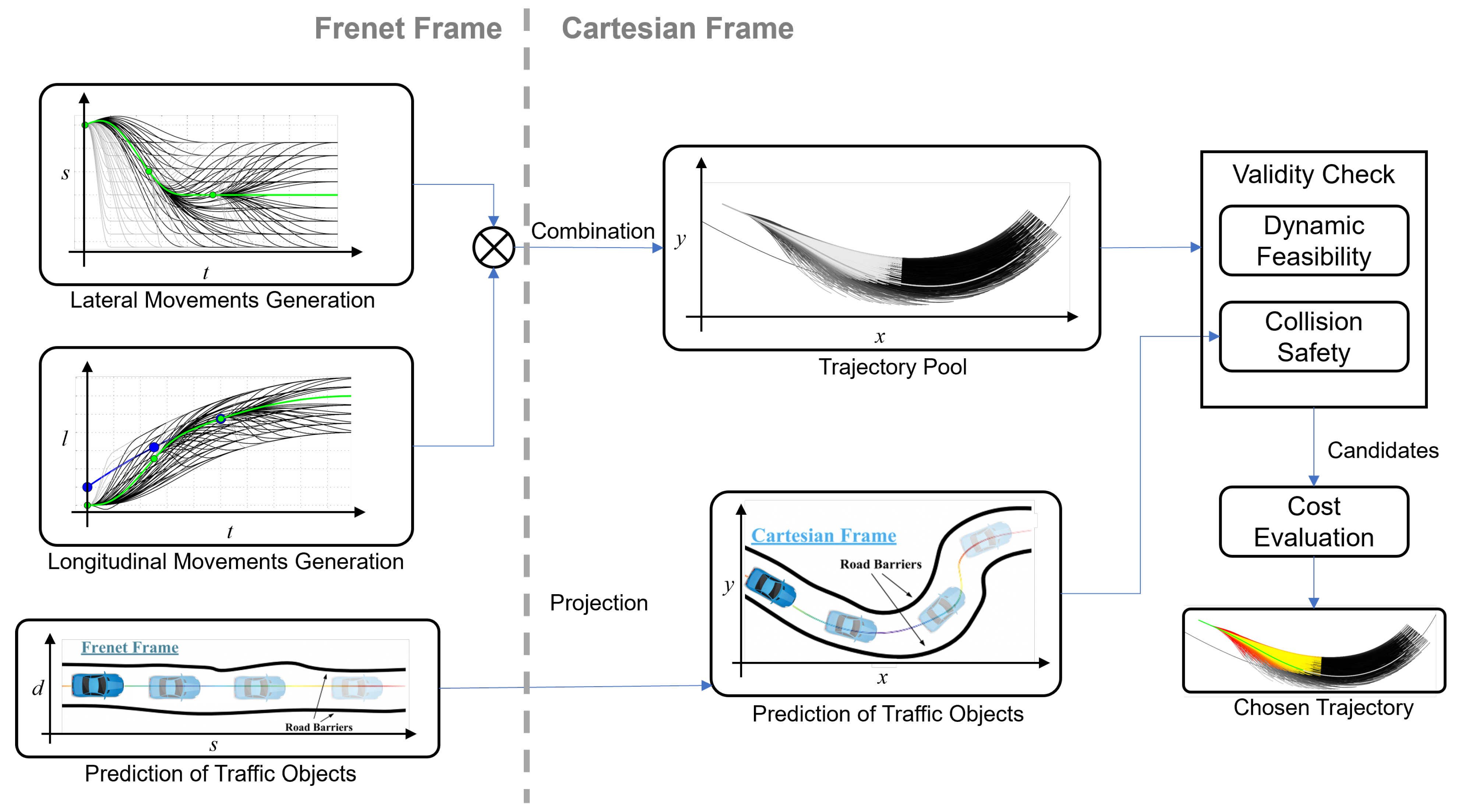
  • Generation of Candidate Trajectories in the Frenet Frame: Quintic polynomials are generated for both the lateral and longitudinal motion in the Frenet coordinate system. The Frenet frame represents the vehicle’s motion along the curvilinear road geometry, where the lateral and longitudinal dimensions are decoupled. These polynomials capture various driving behaviors, such as maintaining velocity, following, merging, or stopping. The polynomials are then combined to form a set of candidate trajectories, which are transformed into the Cartesian frame for further analysis.
  • Object Representation and Prediction: Traffic objects, such as other vehicles, are also represented in the Frenet frame per lane. This simplifies the prediction of their future movements, as road geometry is straightened in this frame. For instance, models like the Intelligent Driver Model (IDM) can be applied to predict object motion, which is then converted back into the Cartesian frame.
  • Feasibility and Collision Checks: The generated candidate trajectories are subjected to the two following checks: (1) dynamic feasibility, ensuring that the trajectories are physically realizable by the ego vehicle, and (2) collision checks in the Cartesian frame, where box-based safety checks are performed, considering the shapes and predicted positions of both the ego vehicle and surrounding objects.
  • Cost Evaluation and Optimal Trajectory Selection: The remaining feasible trajectories are evaluated using a cost function. This function accounts for factors such as collision risk, efficiency, driving comfort, and deviation from the centerline. The trajectory with the lowest cost is selected as the final, optimal path for the vehicle to follow.
The trajectory pool is generated within the Frenet frame for each lane, providing the vehicle with the flexibility to select the most suitable trajectory from among different lanes. This approach proves advantageous in dynamic scenarios involving unexpected road obstacles, as it allows the vehicle to switch to feasible trajectories in alternative lanes if those in the current lane prove suboptimal or unviable [28,38]. Additionally, a cost associated with lane changes is incorporated into the evaluation to penalize frequent lane switching, thereby promoting stability and safety in the vehicle’s navigation strategy.
To simplify the validation pipeline, the control module is not included, and hence the tracking errors are not included in the discussion. As previously noted, the proposed local planning method is decoupled from the downstream control module, and thus, this simplification will not impact the final results. Instead, it is assumed that the trajectory is executed based on the corresponding timestamps during execution.
The estimation error of the state change is partly because of measurement errors from the sensors. The following measurement models are assumed for vehicle speed, derived from wheel speed sensors, and yaw rate, obtained from the yaw rate sensor:
v m = v offset + v ˜ , where v ˜ N ( v , σ v ) .
θ ˙ m = θ ˙ offset + θ ˙ ˜ , where θ ˙ ˜ N ( θ ˙ , σ θ ˙ ) .

3. Stability Analysis

3.1. Problem Description

Equations (3) and (4) give an approximation of the relative motion change between consecutive planning timesteps. However, due to the integrals in the equations, the estimation of vehicle position and posture changes since the first timestep could build up as time progresses. The accumulated error could have adverse effects on the proposed local trajectory planning method, making it infeasible to reach the desired destination.
To simply the analysis, the terminal destination x f of the trajectory planning for consecutive timesteps is assumed unchanged in order to show the stability concept for continuous planning. This simplification is feasible for consecutive timesteps in scenarios like traffic stop, lane changing, etc.
The diagram in Figure 3 illustrates the potential effect of the accumulated estimation error on the continuous trajectory planning results at timestep t k 1 and the subsequent timestep t k . To clearly demonstrate the drift of the trajectory due to the estimation error, the trajectories T k 1 and T k , planned in their respective local coordinate systems, are represented under the same global coordinate system, where the terminal destination is set to 0 .
Figure 3a shows that without an estimation error of the state change, trajectory T k ’s start point x k | T k has the same state as the planned next-timestep state x k | T k 1 by last trajectory T k 1 , which is the prerequisite to realize the consistency of planning between timesteps. This can be proved as follows. From Equation (1), we have
x k | T k 1 P k = x k | T k 1 P k 1 P k P k 1 ,
x ^ k | T k 1 P k = x k | T k 1 P k 1 Δ P ^ k ,
The estimation error of the state change between neighboring timesteps thus comes from:
ε = P k P k 1 Δ P ^ k .
In the case of Figure 3a, when estimation error ε = 0 , Δ P ^ k = P k P k 1 . In this case, x ^ k | T k 1 , used as the initial planning start state x k | T k at time t k , has the following relationship:
x k | T k = x ^ k | T k 1 = x k | T k 1 .
In the case og ε 0 in (9), minus Equation (7) from (8), we have:
x ^ k | T k 1 P k = x k | T k 1 P k + ( P k 1 P k Δ P ^ k ) ,
= x k | T k 1 P k + ε ,
and therefore
x ^ k | T k 1 = x k | T k 1 + ε ,
under the global coordinate system.
Under this case in Figure 3b, the start state x k | T k for T k deviates from the planned next-timestep state x k | T k 1 at T k 1 . The deviation between x k | T k and x k | T k 1 is exactly the estimation error ε of state change.
Also note that both trajectories lead to the same terminal state x f despite the existence of the error term ε . This is because the terminal state is assumed fixed for stability analysis purposes, as mentioned before. Although different local vehicle coordinate systems are used to represent the terminal state at each timestep during planning, i.e., x f P k 1 vs. x f P k , the coordinate transformation itself does not change any global object’s state, including x f . Hence, x f is not affected by the estimation error ε of state change, and every trajectory at each timestep attempts to reach this destination x f .
It is likely that under the case Figure 3b, if the error term ε is large enough, the continuously planned trajectory may never converge to the terminal state x f , as ε may drag the planning start point further and further away from x f . This inference is intuitive but lacks theoretical support. The questions of interest are as follows: Is the terminal state reachable during continuous planning, given the estimation error ε of state change? What are the permissible bounds for ε ?

3.2. Stability Analysis

In the presence of estimation error ε , it is proven in last subsection that:
x k | T k = x ^ k | T k 1 = x k | T k 1 + ε ,
  = x k 1 | T k 1 + Δ x k | T k 1 Planned   state   change at   trajectory   T k 1 +   ε   Estimation   error   of the   state   change ,
as illustrated in Figure 3b.
Denote x k | T k by x k in the above equation, then we have the following discrete-time system, described by:
x k = f ( x k 1 ) = x k 1 + Δ x k | T k 1 + ε
= x k 1 + Δ x k | ρ k 1 ,
where f : D R is locally Lipschitz in D R 3 , and D is an open set containing the origin 0 D .
The stability problem of the continuously trajectory planning then becomes the stability analysis for the discrete-time orbit, i.e., the sequence of state x k starting from an initial state x 0 .
Suppose f has an equilibrium at x f = 0 ; then, the equilibrium 0 is said to be locally Lyapunov stable if:
  • For every r > 0 , there exists a δ > 0 , such that, if x 0 0 < δ , then x k 0 < r for every k > = 0 .
Figure 4 shows an exemplary sequence of discrete state x ( · ) confined in the open ball of radius r, B r = { x R 3 x < r } , projected in a 2D plane.
Define a Lyapunov-alike function V : D R locally Lipschitz in D with the form:
V ( x ) = x T x , x D ,
which satisfies the following properties:
V ( 0 ) = 0 , and V ( x ) > 0 , x D 0 .
Given the ( k 1 ) -th state x k 1 , the value change of function V : D R from x k 1 to x k is:
Δ V ( x k 1 ) = V ( f ( x k 1 ) ) V ( x k 1 )
= x k 1 + ρ k 1 T x k 1 + ρ k 1 x k 1 T x k 1
= 2 x k 1 + ρ k 1 T ρ k 1 .
The following prerequisite is assumed to be satisfied for Δ V ( x k 1 ) :
Prerequisite 1. 
η > 0 , such that x k 1 { x D x > η } , Δ V ( x k 1 ) 0 is always satisfied, given the Lipschitz-continuous function V : D R defined in Equations (18) and (19).
Remark 1. 
Prerequisite 1 is not stringent in the context of the continuous trajectory planning problem. It will be demonstrated in the following that, under certain easily met conditions, the assumed prerequisite can be ensured.
To satisfy Δ V ( x ) 0 , from Equation (22) the inner product of ( 2 x + ρ ) and ρ have to be no greater than 0. Figure 5 shows the physical meaning of this in the Euclidean plane. It shows different possibilities of ρ and how it affects the 2 x + ρ and, correspondingly, their inner product.
Of the three examples given in the figure, either ρ is too long or a wrong direction leads to 2 x + ρ · ρ > 0 . It is straightforward that two conditions have to be met to satisfy the non-positive inner product in Euclidean plane: (1) ρ · x 0 ; and (2) ρ should be less than the projection of 2 x on ρ . For the vector space R 3 , similarly, it is concluded that the following conditions have to be satisfied to ensure Δ V ( x ) 0 :
x T ρ 0 , and ρ T ρ < 2 x T ρ .
It will be demonstrated in the following discussion that condition (23) can be met. The term ρ contains the estimation error of state change, ε , as seen from Equations (15) and (17). The error ε is in probabilistic distribution due to noise and error from the motion sensors. Sensor noise and error is usually small and hence it is safe to assume a upper bound that:
  • ε ¯ , such that ε is bounded ε < ε ¯ .
The other term contained in ρ is Δ x k | T k 1 , which is the planned next-step state change at T k 1 . Figure 6 shows a possible vector of Δ x k | T k 1 given the ( k 1 ) -th step’s planning initial point x k 1 under Euclidean plane as an example. Due to the nature of trajectory planning, the planned trajectory steps towards the terminal state 0 . Consequently, the following relation may be assumed:
Δ x k | T k 1 T x k 1 < 0 .
In Figure 6, the open ball of radius ε ¯ is shown in the grey shaded area atop the tip of Δ x k | T k 1 . Then, the vector ρ , i.e., the sum of Δ x k | T k 1 and ε , is known to be confined in this shaded area. If for any ε that is bounded in ε < ε ¯ , the condition (23) could be satisfied, then Δ V ( x ) 0 can be guaranteed.
This is very likely to be satisfied when the error bound ε ¯ is significantly smaller compared to the norm x k 1 or Δ x k | T k 1 if the relation (24) is met. Consequently, it can be assumed that η > 0 , for any x k 1 D that satisfies x k 1 > η , condition (23) is always met, and hence Δ V ( x k 1 ) 0 . The above discussion shows how the Prerequisite 1 is made.
Prerequisite 2. 
In the discrete system (17), ρ is bounded within an open ball with radius ρ ¯ , i.e., ρ < ρ ¯ .
Proof. 
During planning, the vehicle’s own physical motion capabilities would be considered to limit the planned state change Δ x k | T k 1 , i.e.,
Δ x k | T k 1 < Δ x ¯ .
And hence,
ρ Δ x k | T k 1 + ε < Δ x ¯ + ε ¯
Therefore, there must exist a ρ ¯ , such that ρ < ρ ¯ and ρ ¯ Δ x ¯ + ε ¯ . □
Remark 2. 
For the trajectory planning problem, the terminal state x f = 0 may not be an equilibrium point, since f ( 0 ) = 0 is not guaranteed due to the term ρ in Equation (17). However, according to Prerequisite 2, it is known that the next state from 0 is in close proximity, i.e., f ( 0 ) ρ ¯ .
Claim 1. 
For the discrete system described in Equation (17), with Prerequisites 1 and 2, the Lyapunov stability could not be achieved; but a weaker conclusion could be drawn: there exists a δ > 0 , if x 0 0 < δ , then x k is bounded in the sense that x k 0 < r for every k 0 for some r.
Proof. 
Choose s = m a x η , ρ ¯ where η and ρ ¯ are declared in Prerequisites 1 and 2, such that the open ball B s = x R 3 x < s D . Then, choose r > s + ρ ¯ > 0 that B r = x R 3 x < r D . Let α = min x = r V ( x ) , then we know α > 0 due to (19). Take β ( 0 , α ) , the set Ω β = B r V 1 ( [ 0 , β ] ) B r could have several connected components, as indicated in Figure 7.
Consider C β Ω β is the connected component that contains B s , i.e., B s C β . Since the function has the same form as in (19), this can be ensured with a chosen β ( s + ρ ¯ ) 2 . In the following, it will be proven that f n ( C β ) C β for every n 0 .
First, it is demonstrated that the next discrete state from 0 remains within C β , i.e., f ( 0 ) C β . According to Prerequisite 2, it follows that f ( 0 ) < ρ ¯ s . Thus, f ( 0 ) B s C β .
Next, we prove that f ( C β ) B r V 1 ( [ 0 , β ] ) . This has to be discussed for B s and C β B s separately. For x B s ,
f ( x ) x + ρ < s + ρ ¯ < r ,
and hence,
f T ( x ) f ( x ) < ( s + ρ ¯ ) 2 β .
Therefore, f ( B s ) B r V 1 ( [ 0 , β ] ) .
Then, since f : D R 3 is Lipschitz in D, f ( C β ) is also connected and f ( B s ) f ( C β ) . This implies that at least a portion of f ( C β B s ) is also a subset of B r . It can further be concluded that f ( C β B s ) B r . If this is not true, then f ( C β B s ) overlaps with B r . There is a point x C β B s such that f ( x ) = r . Then, the Lyapunov-alike function
V ( f ( x ) ) α > β V ( x ) .
This is contradictory to the non-increasing characteristics of V ( x ) in Prerequisite 1.
Thus, f ( C β ) is connected and a subset in B r V 1 ( [ 0 , β ] ) . Meanwhile, f ( 0 ) f ( C β ) and f ( 0 ) C β . This implies that f ( C β ) C β . Consequently, it can be concluded that f n ( C β ) C β for any n N . Therefore, a δ > 0 can be chosen such that x D x < δ C β , if x < δ , then f n ( x ) < r . □
Claim 2. 
If Δ V ( x ) is strictly decreasing in Prerequisite 1, for the system (17) along with Prerequisite 2, there exists δ > 0 , such that if x 0 0 < δ , then lim n x n 0 < η + ρ ¯ . This means that the state x k will be contained in B η + ρ ¯ = { x D x < η + ρ ¯ } at some point, and its orbit will remain inside thereafter.
Proof. 
From the proof part for Claim 1, choose the δ that satisfies x D x < δ C β , if x < δ , then f n ( x ) C β for every n 0 .
First, it is shown that for x C β B η , there exists some point, k, such that f k ( x ) B η , where B η = { x D x < η } . For the sake of contradiction, suppose that this is not the case; then, for all k 0 we have
f k ( x ) C β B η .
Since C β B η is compact, and Δ V is continuous and Δ V ( x ) < 0 for x C β B η , then from the Weierstrass theorem, we know Δ V attains a negative maximum μ , i.e.,
Δ V ( x ) μ < 0 , if x C β B η ,
and hence,
  V ( f n ( x ) ) = V ( f n 1 ( x ) ) + Δ V ( f n 1 ( x ) )
      = V ( f n 2 ( x ) ) + Δ V ( f n 2 ( x ) ) + Δ V ( f n 1 ( x ) )
  = V ( x ) + k = 1 n 1 Δ V f k ( x )
V ( x ) ( n 1 ) μ .
Letting n + , the right-hand side tends to . This contradicts V ( x ) > 0 for x D 0 . Therefore, for x C β B η , there must exist some k, such that:
f k ( x ) B η .
For x B η ,
f ( x ) x + ρ
< x + ρ ¯ .
This shows that f ( x ) B η + ρ ¯ if x B η . Together with the summary made in (37), the Claim 2 can be proved. □
Remark 3. 
Claim 2 further extends the boundedness conclusion made in Claim 1, and shows that for the trajectory planning problem, as k + , the planned state will eventually contained in B η + ρ ¯ , despite the state change estimate error. The B η + ρ ¯ is a relatively small area and should satisfy the need for the trajectory planning problem.

4. Results and Discussion

Two scenarios are designed to experiment the local planning method without global positioning information. The simulations of two scenes were conducted with the validation pipeline developed in Section 2.2.
To experiment the effects of sensor drift and noise to the planning results, the measurement errors of the speed and yaw rate sensor in (5) and (6) are set to under normal distributions, with the values of offsets and standard deviations shown in Table 1.
These errors are intentionally set to large values to validate the stability of the proposed local planning methodology. Normally, the speed and yaw rate sensor would achieve more accurate readings with respect to the ground truth.

4.1. Moving Traffic Scene

In this scene, the ego car is set to run in a double-lane road with other moving vehicles. Figure 8 shows the the continuous local planning results under the measurement error settings in Table 1. The moving vehicles are shown in blue bounding boxes, which are enlarged to ensure safe distance is maintained from the ego car. The dashed-line boxes represent the predicted motions for these vehicles. The ego vehicle is represented in a green box in this figure. The candidate trajectory planned for each lane (left lane in blue, right lane in orange) with a planning horizon of 5.0 s is also displayed extended from the tail of the ego vehicle. The selected trajectory is highlighted in red points, with each point representing an increment of 0.1 second per timestep. This helps visualize the speed change by observing the density and spread of the selected trajectory.
In Figure 8, the ego car performs a right lane change first, and then follows the car in front until the gap in the left lane is safe enough for it to make another lane change back to the left lane. The safety distance in both the longitudinal and lateral directions of the ego car are well maintained. The ego car centers well within the lane bounds when not changing lanes. This demonstrates that despite the unavailability of global localization information and the not-so-accurate sensor readings of speed and yaw rate to estimate the relative motion, the continuous planning remains highly feasible under the proposed methodology in Figure 1.
Figure 9 shows the change in the speed and yaw rate of the ego car during the moving traffic scene, as well as the measurement readings in the blue-cross line. The time plots of the measurement errors are also displayed in the right-hand subplots to show the deviation and noise of the sensor readings under the sensor noise settings in Table 1.
It is also examined how the measurement errors from the speed and yaw rate affect the relative motion estimate between the planning timesteps. In Figure 10, the top two plots shows the box plot as well as the scattering of the measurement errors. The bottom plots show how the above measurement errors, which resulted in the estimated errors ε in Equation (9) for the pose change between planning timesteps, i.e., Δ x , Δ y , and Δ θ , under the local coordinate system.

4.2. Stop Scene

Another scene where the vehicle has to stop to wait in traffic was ran with the same measurement error settings for the speed and yaw rate. It is of interest to see how the vehicle will perform under low speed or at static. In this scene, a fixed stop distance was set to observe whether the ego car could reach and maintain the target pose under the impact of measurement errors.
Figure 11 shows that the traffic in both lanes is blocked by a long semi-truck and a sedan in front. The ego car decelerates to a full stop. The bottom subplots demonstrate that the ego car is capable of maintaining the stop pose despite the estimation error of relative motion change between timesteps caused by the sensor errors. Interested readers can refer to the animation (the animation gif is available at https://bit.ly/3sFb1hk, accessed on 22 September 2024) to see how the planning compensates the estimation error and get a sense of how the condition (23) is met under this error setting.
Note that the planned speed is negative in both bottom plots in Figure 11 when the vehicle is stopped. This is due to the fact that negative speed error offset v offset = 0.1 m / s leads to a positive estimation error offset of Δ x along the longitudinal direction, as can be seen in Figure 10. From Equation (13), the planned start point for the next timestep will be further ahead, due to the positive estimation error of the pose change; thus, making the start point being moved back under the local coordinate system.

4.3. Stability Limits at Sensor Offset Errors

As discussed in Section 3, Prerequisites 1 and 2 have to both be satisfied to ensure the stability of the local planning problem, as stated in Claim 2. The experiments were conducted under larger sensor offset errors to check the stability limits for the tested two scenes.
Figure 12 shows the screenshots for the two scenes at a much larger speed measurement offset error, v offset = 1.0 m / s . Figure 12a shows at timestamp 11.5 s, the ego car reaches to a farther position compared to Figure 8 and starts a third lane-change to surpass the vehicle in the left lane. Figure 12b, on the other hand, shows that the ego car keeps creeping forward until it crashes into the front car. This is due to the fact that the estimate error of the pose change between timesteps is too large for the planning motion to compensate, which then gradually accumulated to larger deviations from the target pose, essentially drifting away from the target pose. Claim 2 would not be valid, as the Prerequisite 2 is not satisfied under such cases.
Figure 13 are time frames of the two scenes under yaw rate offset θ ˙ offset of 2.29 deg/s and 5.73 deg/s, respectively. At θ ˙ offset = 2.29 deg / s in Figure 13b, the ego car is not capable of centering itself in the middle of the lane and almost drives on the edge of the right lane compared to Figure 11. Considering that a yaw rate offset of 2.29 deg/s is already abnormally large, it shows that the proposed local planning framework is very robust in maintaining the stability of continuous planning. Under an even larger error θ ˙ offset = 5.73 deg / s in Figure 13c,d, the ego car drifts right so much that it eventually crosses over the lane bound and leads to a potential crash or fails in both scenarios.

5. Conclusions

Overcoming the challenge of Level-2+ semi-autonomous driving without relying on highly accurate absolute localization has been the focal point of this study. This paper has explored the feasibility of local trajectory planning based solely on a vehicle’s local coordinate system, without the need for global localization. The proposed trajectory planning methodology leverages pose change estimation between planning timesteps derived from motion sensors, as well as the relative positions of traffic objects and lane markings with respect to the ego vehicle within this local coordinate framework. Additionally, the stability of the planning method under sensor errors was modeled as a Lyapunov stability problem, with the stability proven under certain conditions (as discussed in Section 3). A validation pipeline was constructed, simulating two scenarios under varying levels of sensor errors related to speed and yaw rate measurements. The simulation results strongly support the theoretical stability analysis, demonstrating that continuous trajectory planning can function robustly even in the presence of significant sensor noise, as detailed in Table 1 with speed error distribution v err N ( 0.1 , 0.1 ) m/s and yaw rate error distribution θ ˙ err N ( 0.57 , 1.72 ) deg/s.
One major contribution of this paper is the introduction of a local trajectory planning framework that operates without the requirement for absolute localization, addressing a critical challenge in L2+ semi-autonomous driving, where the available hardware is often limited. Another key contribution is the proof that the dynamic trajectory planning method, subject to motion sensor errors, maintains stability under conditions that are practical and feasible for real-world systems. The stability of this approach was further validated through a series of simulations involving sensor drift and offset errors, particularly from IMU sensors. These findings provide valuable insights into the potential of L2+ semi-autonomous driving applications under hardware constraints, presenting a practical approach for future development in this domain.
Despite its contributions, the proposed methodology does have limitations. The assumption of certain noise characteristics in the sensors (as modeled in Table 1) may not fully capture the complexities of real-world sensor behavior, including more extreme or intermittent failures. Moreover, the proposed framework assumes idealized environmental conditions, and further testing is required in more complex, dynamically changing environments involving highly congested traffic or unpredictable road conditions.
Regarding future work, further refinement of the proposed methodology is needed to address these limitations. Extending the validation scenarios to include more dynamic and unstructured environments, as well as integrating more sophisticated models for sensor failure modes, would offer a more comprehensive evaluation of the system’s robustness. Future research could also explore real-world deployment and testing to evaluate the practical application of this framework in mass-market vehicles with cost-sensitive hardware setups.

Author Contributions

Conceptualization, S.Z. and B.A.-G.; Methodology, S.Z., J.W., Y.Y. and B.A.-G.; Software, S.Z.; Validation, S.Z.; Formal analysis, S.Z.; Investigation, S.Z., J.W., Y.Y. and B.A.-G.; Resources, B.A.-G.; Writing—original draft, S.Z.; Writing—review & editing, J.W., Y.Y. and B.A.-G.; Visualization, S.Z.; Supervision, B.A.-G.; Project administration, B.A.-G. All authors have read and agreed to the published version of the manuscript.

Funding

This research received no external funding.

Data Availability Statement

Data is contained within the article.

Acknowledgments

The authors thank the Automated Driving Lab at the Ohio State University.

Conflicts of Interest

The authors declare no conflict of interest.

References

  1. Dave, P. Dashcam Footage Shows Driverless Cars Clogging San Francisco. 2023. Available online: https://www.wired.com/story/dashcam-footage-shows-driverless-cars-cruise-waymo-clogging-san-francisco/ (accessed on 12 April 2023).
  2. Metz, C. Self-Driving Car Services Want to Expand in San Francisco Despite Recent Hiccups. 2023. Available online: https://www.nytimes.com/2023/02/01/technology/self-driving-taxi-san-francisco.html (accessed on 12 April 2023).
  3. Korosec, K. Uber Spent $457 Million on Self-Driving and Flying Car R&D Last Year. 2019. Available online: https://techcrunch.com/2019/04/11/uber-spent-457-million-on-self-driving-and-flying-car-rd-last-year/ (accessed on 12 April 2023).
  4. Korosec, K. Ford, VW-Backed Argo AI Is Shutting Down. 2022. Available online: https://techcrunch.com/2022/10/26/ford-vw-backed-argo-ai-is-shutting-down/ (accessed on 12 April 2023).
  5. Hirsch, J. Financial Challenges Shutter Self-Driving Truck Company Embark Technology. 2023. Available online: https://www.autonews.com/mobility-report/embark-technology-shuts-down (accessed on 12 April 2023).
  6. Thorbecke, C. Alphabet’s Self-Driving Car Unit Has Cut 8% of Its Staff This Year. 2023. Available online: https://www.cnn.com/2023/03/01/tech/waymo-layoffs/index.html (accessed on 12 April 2023).
  7. Neill, C. TuSimple to Lay Off 25% of Workforce. 2022. Available online: https://www.reuters.com/business/autostransportation/tusimple-lay-off-25-workforce-2022-12-21/ (accessed on 12 April 2023).
  8. Kolodny, L. Tesla Reports Record Revenue and Beats on Earnings. 2023. Available online: https://www.cnbc.com/2023/01/25/tesla-tsla-earnings-q4-2022.html (accessed on 12 April 2023).
  9. O’Hare, B. Tesla Reveals How Many Buyers Have Bought FSD. 2023. Available online: https://insideevs.com/news/629094/tesla-how-many-buy-fsd/ (accessed on 12 April 2023).
  10. Gassée, J.L. Tesla vs. Waymo. 2019. Available online: https://mondaynote.com/tesla-vs-waymo-762cc6a8771b (accessed on 13 April 2023).
  11. International, S. Taxonomy and definitions for terms related to driving automation systems for on-road motor vehicles. SAE Int. 2018, 4970, 1–5. [Google Scholar]
  12. China L2 and L2+ Autonomous Passenger Car Research Report, 2022; Technical Report 5697800; Research in China: Beijing, China, 2022.
  13. Rosenthal, E. When a Tesla on Autopilot Kills Someone, Who Is Responsible? 2022. Available online: https://www.nyu.edu/about/news-publications/news/2022/march/when-a-tesla-on-autopilot-kills-someone--who-is-responsible--.html (accessed on 13 April 2023).
  14. Ji, X. Why Are L4 Autonomous Driving Firms Delivering L2 Solutions? 2022. Available online: https://equalocean.com/analysis/2022062218310 (accessed on 13 April 2023).
  15. Schütz, A.; Sánchez-Morales, D.E.; Pany, T. Precise positioning through a loosely-coupled sensor fusion of GNSS-RTK, INS and LiDAR for autonomous driving. In Proceedings of the 2020 IEEE/ION position, location and navigation symposium (PLANS), Portland, OR, USA, 20–23 April 2020; pp. 219–225. [Google Scholar]
  16. Yan, Z.; Sun, L.; Krajník, T.; Ruichek, Y. EU long-term dataset with multiple sensors for autonomous driving. In Proceedings of the 2020 IEEE/RSJ International Conference on Intelligent Robots and Systems (IROS), Las Vegas, NV, USA, 24 October 2020–24 January 2021; pp. 10697–10704. [Google Scholar]
  17. Nagai, K.; Spenko, M.; Henderson, R.; Pervan, B. Evaluating INS/GNSS availability for self-driving cars in urban environments. In Proceedings of the 2021 International Technical Meeting of The Institute of Navigation, Online, 25–28 January 2021; pp. 243–253. [Google Scholar]
  18. Chalvatzaras, A.; Pratikakis, I.; Amanatiadis, A.A. A survey on map-based localization techniques for autonomous vehicles. IEEE Trans. Intell. Veh. 2022, 8, 1574–1596. [Google Scholar] [CrossRef]
  19. Wang, L.; Zhang, Y.; Wang, J. Map-based localization method for autonomous vehicles using 3D-LIDAR. IFAC-PapersOnLine 2017, 50, 276–281. [Google Scholar] [CrossRef]
  20. Stachniss, C.; Leonard, J.J.; Thrun, S. Simultaneous localization and mapping. In Springer Handbook of Robotics; Springer: Cham, Switzerland, 2016; pp. 1153–1176. [Google Scholar]
  21. Kummerle, R.; Hahnel, D.; Dolgov, D.; Thrun, S.; Burgard, W. Autonomous driving in a multi-level parking structure. In Proceedings of the 2009 IEEE International Conference on Robotics and Automation, Kobe, Japan, 12–17 May 2009; pp. 3395–3400. [Google Scholar]
  22. Qin, T.; Chen, T.; Chen, Y.; Su, Q. Avp-slam: Semantic visual mapping and localization for autonomous vehicles in the parking lot. In Proceedings of the 2020 IEEE/RSJ International Conference on intelligent robots and systems (IROS), Las Vegas, NV, USA, 24 October 2020–24 January 2021; pp. 5939–5945. [Google Scholar]
  23. Singandhupe, A.; La, H.M. A review of slam techniques and security in autonomous driving. In Proceedings of the 2019 Third IEEE International Conference on Robotic Computing (IRC), Naples, Italy, 25–27 February 2019; pp. 602–607. [Google Scholar]
  24. Zheng, S.; Wang, J.; Rizos, C.; Ding, W.; El-Mowafy, A. Simultaneous localization and mapping (slam) for autonomous driving: Concept and analysis. Remote Sens. 2023, 15, 1156. [Google Scholar] [CrossRef]
  25. Brossard, M.; Bonnabel, S. Learning wheel odometry and IMU errors for localization. In Proceedings of the 2019 International Conference on Robotics and Automation (ICRA), Montreal, QC, Canada, 20–24 May 2019; pp. 291–297. [Google Scholar]
  26. Aqel, M.O.; Marhaban, M.H.; Saripan, M.I.; Ismail, N.B. Review of visual odometry: Types, approaches, challenges, and applications. SpringerPlus 2016, 5, 1897. [Google Scholar] [CrossRef] [PubMed]
  27. Zhu, S.; Gelbal, S.Y.; Aksun-Guvenc, B. Online quintic path planning of minimum curvature variation with application in collision avoidance. In Proceedings of the 2018 21st International Conference on Intelligent Transportation Systems (ITSC), Maui, HI, USA, 4–7 November 2018; pp. 669–676. [Google Scholar]
  28. Guvenc, L.; Aksun-Guvenc, B.; Zhu, S.; Gelbal, S.Y. Autonomous Road Vehicle Path Planning and Tracking Control; John Wiley & Sons: Hoboken, NJ, USA, 2021. [Google Scholar]
  29. Ji, Y.; Ni, L.; Zhao, C.; Lei, C.; Du, Y.; Wang, W. TriPField: A 3D potential field model and its applications to local path planning of autonomous vehicles. IEEE Trans. Intell. Transp. Syst. 2023, 24, 3541–3554. [Google Scholar] [CrossRef]
  30. Ma, L.; Xue, J.; Kawabata, K.; Zhu, J.; Ma, C.; Zheng, N. Efficient Sampling-Based Motion Planning for On-Road Autonomous Driving. IEEE Trans. Intell. Transp. Syst. 2015, 16, 1961–1976. [Google Scholar] [CrossRef]
  31. Zhu, S.; Aksun-Guvenc, B. Trajectory planning of autonomous vehicles based on parameterized control optimization in dynamic on-road environments. J. Intell. Robot. Syst. 2020, 100, 1055–1067. [Google Scholar] [CrossRef]
  32. Dolgov, D.; Thrun, S.; Montemerlo, M.; Diebel, J. Path planning for autonomous vehicles in unknown semi-structured environments. Int. J. Robot. Res. 2010, 29, 485–501. [Google Scholar] [CrossRef]
  33. Chen, J.; Zhan, W.; Tomizuka, M. Constrained iterative lqr for on-road autonomous driving motion planning. In Proceedings of the 2017 IEEE 20th International conference on intelligent transportation systems (ITSC), Yokohama, Japan, 16–19 October 2017; pp. 1–7. [Google Scholar]
  34. Tsukamoto, H.; Chung, S.J. Learning-based Robust Motion Planning With Guaranteed Stability: A Contraction Theory Approach. IEEE Robot. Autom. Lett. 2021, 6, 6164–6171. [Google Scholar] [CrossRef]
  35. Englot, B.; Johannsson, H.; Hover, F. Perception, stability analysis, and motion planning for autonomous ship hull inspection. In Proceedings of the International Symposium on Unmanned Untethered Submersible Technology (UUST), Durham, NH, USA, 23–26 August 2009. [Google Scholar]
  36. Gu, T.; Atwood, J.; Dong, C.; Dolan, J.M.; Lee, J.W. Tunable and stable real-time trajectory planning for urban autonomous driving. In Proceedings of the 2015 IEEE/RSJ International Conference on Intelligent Robots and Systems (IROS), Hamburg, Germany, 28 Septembe–2 October 2015; pp. 250–256. [Google Scholar] [CrossRef]
  37. Kant, K.; Zucker, S.W. Toward efficient trajectory planning: The path-velocity decomposition. Int. J. Robot. Res. 1986, 5, 72–89. [Google Scholar] [CrossRef]
  38. Werling, M.; Kammel, S.; Ziegler, J.; Gröll, L. Optimal trajectories for time-critical street scenarios using discretized terminal manifolds. Int. J. Robot. Res. 2012, 31, 346–359. [Google Scholar] [CrossRef]
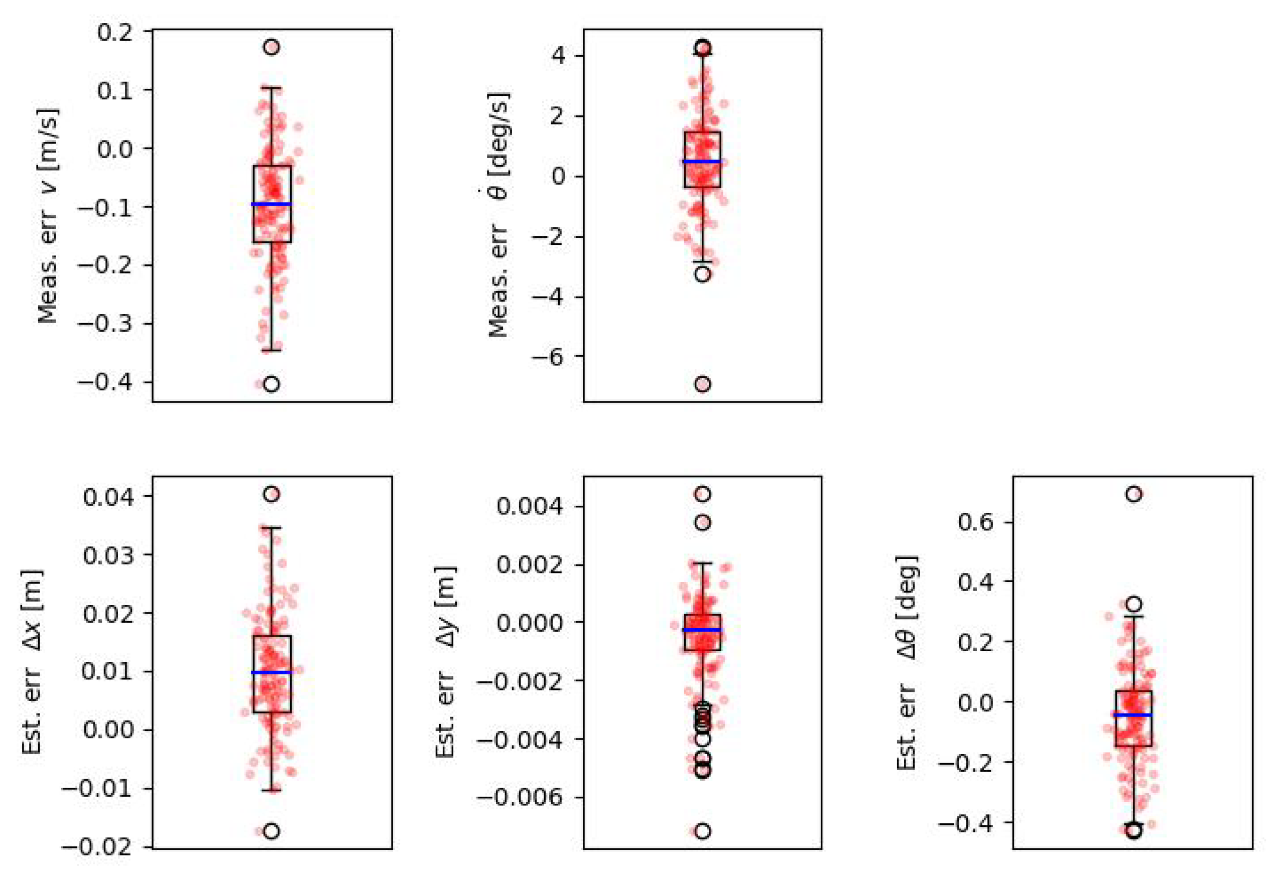
Figure 1. Proposed local trajectory planning framework for Level-2+ semi-autonomous driving without absolute localization.
Electronics 13 03808 g001
Figure 2. The sampling-based local trajectory planning method under the Frenet frame [38] used in the validation pipeline.
Electronics 13 03808 g002
Figure 3. An illustration of the effects of an estimation error of state change ε on continuous planning results at timestep t k 1 and t k .
Electronics 13 03808 g003
Figure 4. Stability in the sense of Lyapunov for discrete-time system projected in 2D plane.
Electronics 13 03808 g004
Figure 5. Inner product of ρ and 2 x + ρ at different combinations in Euclidean plane.
Electronics 13 03808 g005
Figure 6. Example of Δ x k | T k 1 and bounds of ε in Euclidean plane.
Electronics 13 03808 g006
Figure 7. Illustration of the sets’ projection to 2D plane.
Electronics 13 03808 g007
Figure 8. Local planning in a moving traffic scene (The animation gif is available at https://bit.ly/3L4QSHB, accessed on 22 September 2024).
Electronics 13 03808 g008
Figure 9. Time plots of vehicle speed, yaw rate and measurement errors under settings in Table 1.
Electronics 13 03808 g009
Figure 10. Box plots of measurement errors (upper plots) and the resulted estimation errors of relative motion between planning timesteps (bottom plots) under settings in Table 1.
Electronics 13 03808 g010
Figure 11. Local planning in a stop scene (The animation gif is available at https://bit.ly/47XMcxg, accessed on 22 September 2024).
Electronics 13 03808 g011
Figure 12. Effects of significant speed offset error: v err N ( 1.0 , 0.1 ) m / s . (a) Traffic scene at v offset = −1.0 m/s (The animation gif is available at https://bit.ly/3EqyTb4, accessed on 22 September 2024). (b) Stop scene at v offset = −1.0 m/s (The animation gif is available at https://bit.ly/3sAavkt, accessed on 22 September 2024).
Electronics 13 03808 g012
Figure 13. Effects of significant yaw rate offset error at (a,b): θ ˙ err N ( 2.29 , 1.72 ) deg / s ; (c,d) θ ˙ err N ( 5.73 , 1.72 ) deg / s . (a) (Traffic scene at θ ˙ offset = 2.29 deg/s (The animation gif is available at https://bit.ly/3qRgSj7, accessed on 22 September 2024). (b) (Stop scene at θ ˙ offset = 2.29 deg/s (The animation gif is available at https://bit.ly/3P4hMAT, accessed on 22 September 2024). (c) (Traffic scene at θ ˙ offset = 5.73 deg/s (The animation gif is available at https://bit.ly/3ErwE7e, accessed on 22 September 2024). (d) (Stop scene at θ ˙ offset = 5.73 deg/s (The animation gif is available at https://bit.ly/44DSjUB, accessed on 22 September 2024).
Electronics 13 03808 g013
Table 1. Experimental settings of measurement errors.
MeasurementsError Distribution
Speed v v err N ( 0.1 , 0.1 ) m/s
Yaw rate θ ˙ θ ˙ err N ( 0.57 , 1.72 ) deg/s
Disclaimer/Publisher’s Note: The statements, opinions and data contained in all publications are solely those of the individual author(s) and contributor(s) and not of MDPI and/or the editor(s). MDPI and/or the editor(s) disclaim responsibility for any injury to people or property resulting from any ideas, methods, instructions or products referred to in the content.

