Active Power Dispatch of Renewable Energy Power Systems Considering Multiple Renewable Energy Station Short-Circuit Ratio Constraints

Abstract

Active power dispatch of new energy refers to an effective method of ensuring the stable operation and optimal economic benefits of new energy power systems through scientific and rational planning and control of active power output from new energy generation. However, as the proportion of new energy increases, the system’s voltage support capacity decreases, leading to potential voltage collapse and oscillation issues. The Multiple Renewable Energy Station Short-Circuit Ratio (MRSCR) is a critical indicator of the system’s voltage support capacity for power systems with high new energy penetration. This study aims to introduce MRSCR constraints into the active power dispatch to guarantee sufficient grid integration strength and stable operation. The MRSCR constraints are approximated using the least squares fitting method. Additionally, this study compares the economic benefits and margin of the indicators between wind and thermal power active scheduling models with and without considering MRSCR. Case studies show that the active scheduling model considering MRSCR constraints improves the MRSCR margin with minimal loss of economic benefits.

1. Introduction

In the Chinese power grid, large-scale integration of new energy generation equipment, represented by wind and photovoltaic power, has taken place [1]. By the end of 2023, a regional grid in China had added 11.87 million kilowatts of wind and photovoltaic power generation capacity, an increase of 32% year-on-year. Currently, the installed capacity of new energy generation in this regional grid has surpassed 50 million kilowatts, accounting for 76% of the total power capacity. In 2023, the new energy generation in this grid reached 82 billion kilowatt-hours, a year-on-year increase of 14.7%, accounting for 51% of the total power generation. Most existing new energy generation equipment adopts a control mode that tracks the grid voltage, requiring voltage support from the AC grid [2,3,4]. As the proportion of new energy in the system continues to increase, the weak support capability of new energy units causes a continuous decline in the voltage support capacity of the grid. This has led to scenarios where new energy is integrated into a weak AC grid in some regions [5], posing risks to the safe and stable operation of the power system. The focus has thus shifted to ensuring safe and economic dispatch in high-proportion new energy scenarios.

In recent years, scholars, both domestically and internationally, have extensively studied the optimization and dispatch of new energy. Reference [6] studied power dispatch for renewable energy integration based on Reinforcement Learning (RL), aiming to maximize economic benefits and minimize carbon emissions. It focuses on the generation side of the power system and does not consider the impact of the transmission and distribution systems. A cooperative game based on an Integrated Energy System (IES) optimization operation model is proposed in [7], aiming to further optimize the energy utilization rate and operating costs of the comprehensive energy system. It considers cold, heat, electricity, and gas energy; lacking the application and use of new energy sources such as wind power and photovoltaics. The challenge of grasping carbon emission costs across different scheduling periods on multiple time scales is considered in reference [8], aiming to consider carbon emissions and economic benefits of the power system across multiple time scales. The study did not address other environmental impacts. Some scholars proposed a stochastic optimization model based on chance-constrained programming to determine the short-term operational scheduling of a hydro-photovoltaic hybrid energy system, aiming to maximize system power generation efficiency by considering the costs and losses of hydro and photovoltaic power generation [9,10]. It fails to consider the intrinsic impact mechanism of residual load fluctuations influenced by variations in daily average runoff under different typical weather conditions. References [11,12] combined Machine Learning (ML) probabilistic forecasting with robust optimization, aiming to propose a hydrogen refueling station model that relies on integrated hydrogen production and refueling from new energy. The hydrogen refueling station model mentioned in the article does not address the scalability of hydrogen storage for large systems. Improved power supply and demand mismatch by efficiently aggregating and optimizing control of new energy and demand-side resources, reference [13] used Long Short-Term Memory (LSTM) and Latin Hypercube Sampling to forecast day-ahead wind and photovoltaic power output; constructing a day-ahead optimization scheduling model considering system operating costs, curtailment costs and demand response costs while this article does not address the issue of model accuracy under complex energy and economic factors. Reference [14] introduced the generalized short circuit ratio of operation, which can assess the strength of the AC grid after integrating new energy at any power, providing scheduling strategies for new energy integration on different time scales. It established a multi-time scale for new energy integration scheduling model with the objective function of minimizing dispatch costs. The generalized short circuit ratio of operation may not reflect the physical characteristics of the impact of the interaction between multiple renewable energy stations on the system voltage strength. Most of these studies designed dispatch models to maximize economic benefits and minimize carbon emissions, with some evolving from single-objective to multi-objective optimization and incorporating power system stability. Others expanded from single to multiple time scales; incorporating methods such as machine learning, reinforcement learning, and robust optimization. These models mainly focus on the economic and social benefits of the power system, often neglecting the assessment and improvement of grid safety risks under large-scale new energy integration. By considering factors such as the short-circuit capacity at a point in the power system network, defined as the product of the three-phase short-circuit current and the rated voltage, which indicates the system’s voltage strength, we place more emphasis on the impact of indicators such as short-circuit capacity and short-circuit ratio on the model.

However, large-scale integration of new energy into the grid inevitably weakens grid strength and reduces system adjustability, necessitating consideration of the impact of new energy scheduling on system stability. Reference [15] classified the severity of voltage breakdown events in power systems, predicting and classifying the severity of short-term voltage stability events using Long Short-Term Memory (LSTM) and deep learning Convolutional Neural Networks (CNNs). Reference [16] aimed to determine effective power generation while reducing emissions, voltage deviations, and maintaining transmission line voltage stability, guided by the Monkey King Evolution Algorithm based on multiple trial vectors for control selection, achieving optimal power flow and meeting load demand in cogeneration economic dispatch. Reference [17] constructed a novel power system optimization scheduling model considering frequency-inertia safety constraints, introducing an advanced adiabatic compressed air energy storage system as a storage device for wind power absorption, constraining the system’s wind power limit with the rate of frequency change and steady-state frequency deviation. Reference [18] primarily studies the impact of UPFC, wind power units, and photovoltaic units on system stability. It employs a direct optimization algorithm to design stabilizers for the various generation units in a piecewise coordinated manner. Reference [19], based on an analysis of the causes of wind curtailment in new energy power systems, proposes an optimized operational solution. This involves installing heat stations with electric boilers and thermal storage tanks at heating network nodes to enhance the system’s peak-shaving capability and promote wind power integration. Reference [20] delves into the impact of the degree of connection between wind farms and the main power grid, wind farm output, and the connection method of wind farms on the small disturbance stability of the system. Reference [21] establishes a small disturbance stability mathematical model for asynchronous wind turbines and investigates the small disturbance stability analysis method for power systems after the integration of wind farms, achieving its practical engineering application. As the proportion of installed new energy capacity gradually increases, certain regions of the power grid are encountering scenarios where new energy is integrated into weak AC grids, which can lead to issues such as wide-band oscillations and transient overvoltages. These problems affect the safe, stable operation and efficient utilization of new energy. According to China’s mandatory standard, GB38755-2019 [22] “Power System Security and Stability Guidelines”, it is explicitly required that the short-circuit ratio (SCR) of new energy stations should reach a reasonable level. The multi-station short circuit ratio (MRSCR), as a novel SCR metric for evaluating the voltage support strength of the system, helps mitigate the impacts of new energy grid integration and is of great significance in ensuring the safe and stable operation of systems with integrated new energy.

Based on the above analysis, this paper conducts economic dispatch optimization research on the power system of a large-scale new energy cluster using the multi-site short-circuit ratio (MRSCR) index. Under the condition that the MRSCR index is met, the output of thermal power units and wind power units is reasonably arranged to achieve the optimal economic operation of the power system. The arrangement of this paper is as follows: Section 1 introduces the advantages of MRSCR among various short-circuit ratio indicators and linearizes the MRSCR constraints using multivariate least squares fitting combined with formula derivation. Section 2 develops an economic dispatch model for the new energy power system, considering the multi-site short circuit ratio (MRSCR). Section 3 provides examples that solve the new energy dispatch model with and without considering MRSCR, comparing and summarizing the results of these two schemes.

2. Multiple Renewable Energy Stations Short Circuit Ratio Constraint Based on Multivariate Least Squares Fitting

The short circuit ratio (SCR) is an important indicator of system voltage support strength and can clearly assess the impact of new energy grid integration on the power system. In recent years, scholars have been dedicated to proposing more accurate and practical short-circuit ratio indicators. The previously proposed weighted short circuit ratio (WSCR) and composite short circuit ratio (CSCR) [23,24] assume that all power electronic devices are connected at the same AC point, failing to reflect the physical characteristics of the interaction between multiple new energy stations on system voltage strength. The equivalent short circuit ratio (ESCR) and site-dependent short circuit ratio (SDSCR) [25,26] follow the traditional DC short circuit ratio, which neglects the impact of the system equivalent impedance resistance and assumes the same voltage phase angle between stations, failing to reflect the reactive power output of new energy generation equipment and differences in electrical quantity magnitudes and phase angles between nodes within new energy stations. However, the new multiple renewable energy stations’ short circuit ratio (MRSCR) [27] considers the magnitudes and phase differences of electrical quantities between different nodes and can account for the reactive power of new energy generation equipment. It is suitable for evaluating the system voltage strength in various scenarios where multiple new energy stations are integrated.

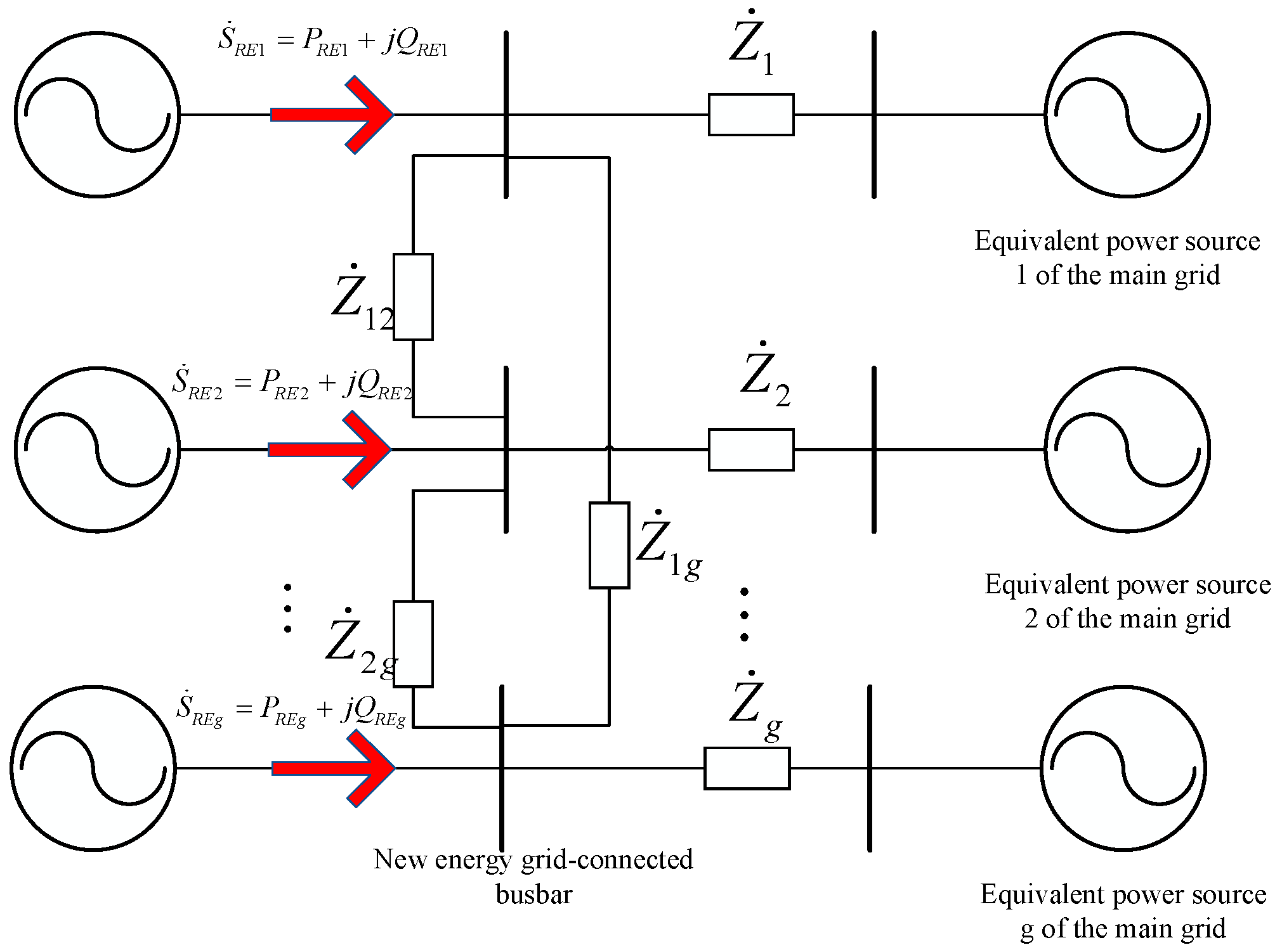
2.1. MRSCR Indicators

Figure 1 is a simplified model of an AC system connected with multiple renewable energy stations. In the figure, ${\dot{S}}_{RE\mathrm{g}}$, $P_{REg}$, $Q_{REg}$ and ${\dot{U}}_{REg}$ represent the apparent power, active power, reactive power, and grid-connected busbar voltage of renewable energy generation station g, respectively. $Z_{gj}$ represents the equivalent impedance between the grid connection points g and j, and $Z_g$ represents the equivalent system-side impedance between the equivalent power source g of the main grid and the corresponding grid connection point.

The short circuit ratio (SCR) measures the relative magnitude between the nominal system voltage and the voltage generated by the equipment after it is connected to the system. Based on the aforementioned physical significance, the MRSCR at the point of connection of the g-th renewable energy unit in the system is given by Equation (1).

$$MRSC{R}_g={\displaystyle \frac{\left|{\dot{U}}_{Ng}\right|}{\left|{\dot{U}}_{REg}\right|}}={\displaystyle \frac{\left|{\dot{U}}_{Ng}\right|}{\left|{\dot{Z}}_{eqgg}{\dot{I}}_g+{\displaystyle \sum _{j=1,j\ne g}^n{\dot{Z}}_{eqgj}{\dot{I}}_j}\right|}}$$

(1)

where ${\dot{U}}_{Ng}$ represents the nominal voltage at the g-th grid connection busbar node; ${\dot{U}}_{REg}$ represents the voltage generated by the renewable energy power at the g-th node, where the subscript RE denotes the renewable energy power station; ${\dot{I}}_g$ and ${\dot{I}}_j$ represents the short-circuit currents provided by the g-th and j-th renewable energy power stations, respectively. ${\dot{Z}}_{eqgg}$ is the self-impedance of node g in the power system, representing the equivalent impedance seen from node g when all other nodes are grounded. ${\dot{Z}}_{eqgj}$ is the mutual impedance between node g and node j in the power system, indicating the ratio of the voltage measured at node j to the current injected at node i.

Let the actual operating voltage of the i-th point of the connection busbar node be ${\dot{U}}_{\mathrm{g}}$, Multiplying both the numerator and the denominator of Equation (13) by $\left|{\dot{U}}_{\mathrm{g}}^{*}/{\dot{Z}}_{eqgg}\right|$, we get:

$$MRSC{R}_g={\displaystyle \frac{\left|{\dot{U}}_g^{*}{U}_{Ng}/{\dot{Z}}_{eqgg}\right|}{\left|{\dot{U}}_g^{*}{\dot{I}}_g+{\displaystyle \sum _{j=1,j\ne g}^n\frac{{\dot{Z}}_{eqgj}}{{\dot{Z}}_{eqgg}}{\dot{U}}_g^{*}{\dot{I}}_j}\right|}}=\left|{\displaystyle \frac{{\dot{U}}_g^{*}{U}_{Ng}}{{\dot{Z}}_{eqgg}}}\right|/\left|{\dot{S}}_{REg}+{\displaystyle \sum _{j=1,j\ne g}^n{\dot{\Pi }}_{gj}{\dot{S}}_{REj}}\right|$$

(2)

where ${\dot{S}}_{REg}$ represents the actual apparent power injected by the g-th renewable energy unit at the point of connection busbar node; ${\dot{\Pi }}_{gj}={\dot{Z}}_{eqgj}{\dot{U}}_g^{*}/{\dot{Z}}_{eqgg}{\dot{U}}_j^{*}$ is the complex power conversion factor between the renewable energy busbars g and j, reflecting the differences in phase and magnitude of electrical quantities between the grid connection points of various renewable energy units/renewable energy stations.

When the resistance is much greater than the reactance, i.e., when X/R > 10, the impact of X/R on the short-circuit ratio is less than 1%. Therefore, in engineering calculations, the resistance part of the system’s equivalent impedance can be neglected. Consequently, the above equation can be simplified to Equation (3).

$$MRSC{R}_g=S_{acg}/(P_{REg}+{\displaystyle \sum _{j\in g,j\ne g}^n{\lambda }_{gj}{P}_{REj}})$$

(3)

where $P_{REg}$ represents the active power injected at the g-th new energy grid connection node, and ${\lambda }_{gj}=\left|Z_{eqgj}/Z_{eqgg}\right|$ is the power conversion factor between the new energy grid connection buses i and j. It reflects the magnitude differences in the equivalent impedance at the grid connection points of various new energy generation devices or new energy power plant grid connection points.

2.2. Constraint Conditions Based on the Short-Circuit Ratio of Multiple Renewable Energy Stations

According to GB38755-2019 “Guidelines for Power System Security and Stability”, the MRSCR at the low-voltage side of the step-up transformer for renewable energy generation units should not be less than 1.5 [27]. Therefore, the MRSCR constraint considered in this paper is given by the following equation:

$$S/(P_{REg}+{\displaystyle \sum _{j\in g,j\ne g}^n{\lambda }_{gj}{P}_{REj}})\ge 1.5$$

(4)

where S and $\lambda$ are constants for a given renewable energy station under the same network topology, while the variable is the active power output of each station. Considering the economic efficiency of the power system, we aim to maximize the output of wind farms and minimize the output of thermal power units. However, the constraint imposed by the MRSCR limits the output of each wind farm, necessitating optimization of the scheduling.

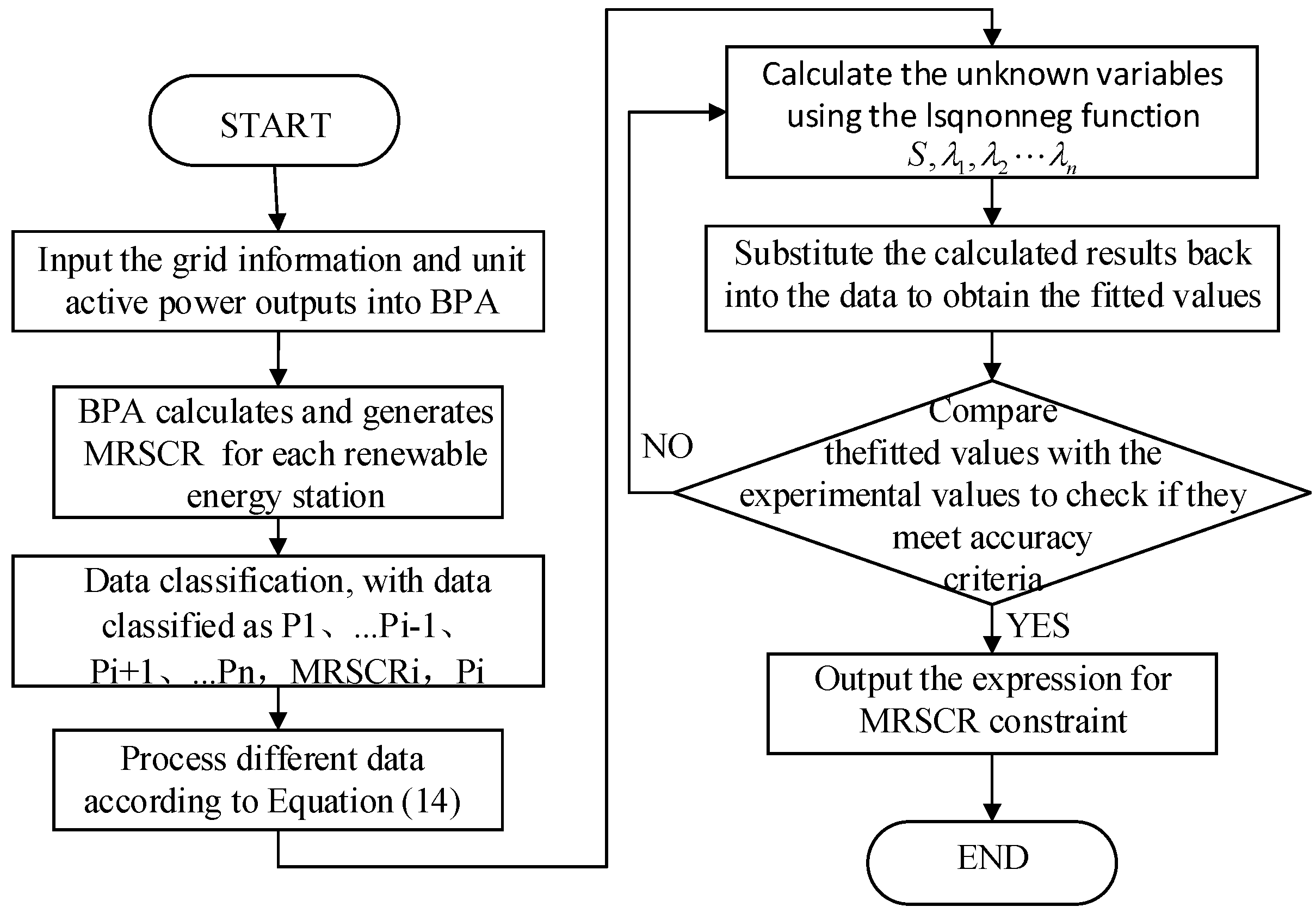
2.3. Multivariate Least Squares Fitting of the MRSCR Constraint

Considering that the MRSCR is closely related to the power output of each renewable energy station in the power system, there must be a set of coefficients that allows the short-circuit ratio to be expressed in terms of active power output. This paper uses multivariate least squares fitting to determine the expression for the MRSCR constraint under the same topology and network configuration.

2.3.1. Multivariate Least Squares Method

Common curve fitting methods include minimizing the sum of absolute deviations (as shown in Equation (5)), minimizing the maximum absolute deviation (as shown in Equation (6)), and minimizing the sum of squared deviations (as shown in Equation (7)).

$$\underset{\phi }{\min }{\displaystyle \sum _{i=1}^m\left|{\delta }_i\right|}={\displaystyle \sum _{i=1}^m\left|\phi (x_i)-y_i\right|}$$

(5)

$$\underset{\phi }{\min } \underset{i}{\max }\left|{\delta }_i\right|=\left|\phi (x_i)-y_i\right|$$

(6)

$$\underset{\phi }{\min }{\displaystyle \sum _{i=1}^m{\delta }_i^2={\displaystyle \sum _{i=1}^m{(\phi (x_i)-y_i)}^2}}$$

(7)

The method of selecting a fitting curve based on the principle of minimizing the sum of squared deviations, using a polynomial equation, is known as the least squares method.

The Multivariate Least Squares Method, often referred as multivariate linear regression, is a statistical technique used to establish linear relationships between multiple independent variables and one or more dependent variables. It is widely used in data fitting, prediction, and analysis due to its ability to quickly and accurately determine linear relationships.

The derivation process is as follows.

Let the fitting polynomial be:

$$y=a_0+a_{1}x+a_2{x}^2+\dots a_k{x}^k$$

(8)

The sum of the distances from each point to this curve, which is the sum of squared deviations, is:

$$R^2={\displaystyle \sum _{i=1}^n{[y_i-(a_0+a_1{x}_i+a_2{x}_i^2+\dots +a_k{x}_i^k)]}^2}$$

(9)

To find the value of coefficients a that meets the conditions, we take the partial derivative of the expression on the right side of the equation with respect to $a_i$. Thus, we obtain

$$\begin{array}{c}-2{\displaystyle \sum _{i=1}^n[y-(a_0+a_{1}x+\dots a_k{x}^k)]=0}\\ -2{\displaystyle \sum _{i=1}^n[y-(a_0+a_{1}x+\dots a_k{x}^k)]x=0}\\ ⋮\\ -2{\displaystyle \sum _{i=1}^n[y-(a_0+a_{1}x+\dots a_k{x}^k)]x^k=0}\end{array}$$

(10)

Simplifying the left side of the equation, we obtain the following equation:

$$\begin{array}{c}{a}_{0}n+a_1{\displaystyle \sum _{i=1}^n{x}_i+}\dots +a_k{\displaystyle \sum _{i=1}^n{x}_i^k}\\ a_0{\displaystyle \sum _{i=1}^n{x}_i}+a_1{\displaystyle \sum _{i=1}^n{x}_i^2+}\dots +a_k{\displaystyle \sum _{i=1}^n{x}_i^{k+1}}\\ ⋮\\ a_0{\displaystyle \sum _{i=1}^n{x}_i^k}+a_1{\displaystyle \sum _{i=1}^n{x}_i^{k+1}+}\dots +a_k{\displaystyle \sum _{i=1}^n{x}_i^{2k}}\end{array}$$

(11)

Express the equation in the following matrix form:

$$\left(\begin{array}{cccc}n& {\displaystyle \sum _{i=1}^n{x}_i}& \cdots & {\displaystyle \sum _{i=1}^n{x}_i^k}\\ {\displaystyle \sum _{i=1}^n{x}_i}& {\displaystyle \sum _{i=1}^n{x}_i^2}& \cdots & {\displaystyle \sum _{i=1}^n{x}_i^{k+1}}\\ ⋮& ⋮& \ddots & ⋮\\ {\displaystyle \sum _{i=1}^n{x}_i^k}& {\displaystyle \sum _{i=1}^n{x}_i^{k+1}}& \cdots & {\displaystyle \sum _{i=1}^n{x}_i^{2k}}\end{array}\right)\left(\begin{array}{c}{a}_0\\ a_1\\ ⋮\\ a_3\end{array}\right)=\left(\begin{array}{c}{\displaystyle \sum _{i=1}^n{y}_i}\\ {\displaystyle \sum _{i=1}^n{x}_i{y}_i}\\ ⋮\\ {\displaystyle \sum _{i=1}^n{x}_i^k{y}_i}\end{array}\right)$$

(12)

Simplifying this Vandermonde matrix, we obtain:

$$\left(\begin{array}{cccc}1& x_1& \cdots & x_1^k\\ 1& x_2& \cdots & x_2^k\\ ⋮& ⋮& \ddots & ⋮\\ 1& x_n& \cdots & x_n^k\end{array}\right)\left(\begin{array}{c}{a}_0\\ a_1\\ ⋮\\ a_k\end{array}\right)=\left(\begin{array}{c}{y}_1\\ y_2\\ ⋮\\ y_n\end{array}\right)$$

(13)

Therefore, the regression coefficient matrix A is given by the following equation:

$$A={(X^{T}X)}^{-1}{X}^{T}Y$$

(14)

2.3.2. Multivariate Least Squares Fitting of the Short-Circuit Ratio Constraint

The short-circuit ratio constraint for multiple renewable energy stations, including those with new energy stations, is easily obtained using the above method. For n renewable energy stations, let the active power output of the i-th station be $P_i$ and the corresponding MRSCR be $MRSC{R}_i$ (calculated online in real-time by the BPA program developed by the China Electric Power Research Institute based on grid information and the active power output of each station).

We can then construct the objective function matrix B, as shown in the following equation.

$$B=[MRSC{R}_i,-x_1,-x_2,\cdots -x_{i-1},-x_{i+1},\cdots -x_n],b=x_i$$

(15)

The regression coefficients are the product of the generalized inverse of matrix B and matrix b. The inversion and multiplication of these matrices can be solved using the lsqnonneg function in MATLAB R2023a. The detailed solution flowchart is shown in Figure 2:

Thus, the overall model is transformed into an optimal power system scheduling problem with the objective function given by Equation (16) and constraints defined by Equations from (17) to Equation (28). The model can then be solved using the Gurobi 11.0.2 solver. Gurobi is a state of the art commercial solver designed for complex mathematical optimization problems and has been widely used in academia and industry. It can efficiently solve linear programming, mixed-integer programming, and other optimization problems.

3. Short-Term Economic Dispatch Model for Wind-Thermal Power Coordination Considering MRSCR

This paper studies a short-term economic dispatch model for a power system with coordinated wind and thermal power generation based on MRSCR constraints. The model aims to maximize the economic benefits of the power system while ensuring that its operation meets various safety and stability constraints; achieving the four fundamental requirements of power systems. Wind power generation is significantly influenced by meteorological conditions, displaying different output characteristics at different times. By leveraging the peak-shaving and valley-filling capabilities of dispatchable thermal power units, the fluctuations in wind power output can be stabilized. At the same time, optimizing the output scheduling of wind power units coordinates the total output of the wind-thermal power system to achieve the best economic benefits. In constructing the dispatch model, this paper aims to make the original output of wind power units fluctuate according to a typical hourly output fluctuation curve for a specific region in China. This curve exhibits distinct time-segmented characteristics, ensuring that the optimized dispatch of the power system is more in line with practical engineering applications.

3.1. Objective Function

This paper establishes the objective function for coordinated wind and thermal power generation: maximizing the economic benefits of power system generation. This involves meeting the power demand at each node while minimizing the production costs within the operational range of the power system. Since wind energy is a renewable and clean energy source, its production costs are significantly lower than those of thermal power, and the shutdown costs of the units are much lower than other costs and can usually be ignored. Therefore, these costs are not considered in our model. The production costs of the power system are primarily determined by the fixed operation and maintenance costs of dispatchable thermal power units, the startup and shutdown costs of generators, the variable costs of fuel consumption, the cost of fuel oil consumption, and the variable operation and maintenance costs.

Thus, the mathematical expression for the objective function is as follows:

$$\min {\displaystyle \sum _{t=1}^T({\displaystyle \sum _g^G(F{C}_g\times O{N}_{g,t}+Ele{c}_{g,t}\times (HeatRat{e}_g\times F{P}_g+V{C}_g)+S{C}_g\times Switc{h}_{g,t})})}$$

(16)

where $F{C}_g$ represents the fixed costs of dispatchable unit g, $F{P}_g$ represents the fuel costs, $V{C}_g$ represents the variable operation and maintenance costs, and $S{C}_g$ represents the startup and shutdown costs of dispatchable unit g. $Ele{c}_{g,t}$ is the power generation of unit g at hour t, and $HeatRat{e}_g$ is the heat rate of unit g. Additionally, $O{N}_{g,t}$ and $Switc{h}_{g,t}$ are two decision variables in the model that describe the operating status of unit g at time t, where $O{N}_{g,t}=1$ indicates that unit g is online at time t, and $Switc{h}_{g,t}=1$ indicates a change in the operating status of unit g at time t. To account for power system operational losses and capacity margins, the model introduces the decision variable voltage angle to estimate the power flow on each transmission line and the decision variables spinning and non-spinning reserves to consider the power system capacity margins.

3.2. Constraints

• Logical constraints on the operational status of dispatchable units:

$$Switc{h}_{g,t}\ge 1-O{N}_{g,t-1}-(1-O{N}_{g,t})$$

(17)

$$O{N}_{g,t}\in \left[0,1\right],Switc{h}_{g,t}\in \left[0,1\right],\forall g,\forall t$$

(18)

Additionally, $O{N}_{g,t}$ and $Switc{h}_{g,t}$ are two binary decision variables in the model that describe the operational status of dispatchable unit g at time t. We can determine the values of these decision variables based on the on/off status of the generator over consecutive hours, and subsequently calculate the startup and shutdown costs of the generator.

2.

Minimum startup and shutdown time constraints for generators:

$$\begin{array}{l}O{N}_{g,t}-O{N}_{g,t-1}\le O{N}_{g,j},\forall g,t\in \left[2,T-1\right]\\ t<j\le \min (t+T_g^{\min -up}-1,T)\end{array}$$

(19)

$$\begin{array}{l}O{N}_{g,t-1}-O{N}_{g,t}\le 1-O{N}_{g,j},\forall g,t\in \left[2,T-1\right]\\ t<j\le \min (t+T_g^{\min -down}-1,T)\end{array}$$

(20)

Minimum startup and shutdown time constraints are crucial in power system scheduling. These constraints ensure that the startup and shutdown times of generators meet their physical and operational requirements, preventing frequent startups and shutdowns that could damage the generators and maintaining system stability. In Equations (19) and (20), the binary decision variables $O{N}_{g,t}$ and $Switc{h}_{g,t}$ are subject to the maximum and minimum startup and shutdown time constraints of the units. They determine the on/off status and changes in the on/off state of each dispatchable unit. Parameter T is defined as the planning horizon. It is the duration of the planning period, measured in hours. $T_g^{\min -up}$, $T_g^{\min -down}$ represent the minimum on-time and minimum off-time, respectively.

3.

Ramp rate limit constraints for generators:

$$Ele{c}_{g,t}-Ele{c}_{g,t-1}\le R{U}_g;\forall g,\forall t$$

(21)

$$Ele{c}_{g,t-1}-Ele{c}_{g,t}\le R{D}_g;\forall g,\forall t$$

(22)

In practical applications, the actual operating range of each generator g within the interval t is constrained by the corresponding ramp rate limit. This is to avoid placing excessive stress on the boilers and combustion equipment and to prevent damage to the generators or instability in the system due to rapid power changes. $R{U}_g$ and $R{D}_g$ are the ramp-up and ramp-down rates of dispatchable unit g, respectively. The overall ramp rate limit constraints can be modeled as shown in Equations (21) and (22).

4.

Maximum and minimum generation capacity constraints for generators:

$$MinCa{p}_g\times O{N}_{g,t}\le Ele{c}_{g,t}\le MaxCa{p}_g\times O{N}_{g,t}\times Derate{F}_{g,t};\forall g,\forall t$$

(23)

The hourly power generation $Ele{c}_{g,t}$ of generator g is constrained by its minimum and maximum generation capacities, as shown in Equation (23). $MinCa{p}_g$ represents the minimum generation power of dispatchable unit g, and $MaxCa{p}_g$ represents the maximum generation power. The term $Derate{F}_{g,t}$ is used to account for the impact of prolonged drought on dispatchable units that rely on freshwater. For example, thermal units may not be able to operate at full capacity due to limited cooling capabilities. Under normal conditions, $DerateF$ is equal to 1.

5.

Power balance constraints:

$$(1-loss)\times {\displaystyle \sum Ele{c}_{n,t}-Deman{d}_{n,t}}+Expor{t}_{n,t}={\displaystyle \sum _{k\in N}LineSu{s}_{n,k}\times (VoltAngl{e}_{n.t}-VoltAngl{e}_{k.t})}$$

(24)

Equation (24) applies to the power balance constraints for each node n connected to any other node k in the power system. The left side of the equation represents the difference between the sum of generation power and incoming power at node n and the network losses and load at n. The right side represents the power flow from node n to all connected nodes k. In this, the power flow variable $VoltAngle$ is a decision variable optimized by the model. The voltage angle of the reference node is set at 0, while the voltage angles of non-reference nodes can be positive or negative. The parameter loss is used to discount the energy production and import, representing the power losses in transmission lines.

6.

Transmission line capacity constraints:

$$-criterio{n}_{N1}\times LineCa{p}_{n,k}\le LineSu{s}_{n.k}\times (VoltAngl{e}_{n,t}-VoltAngl{e}_{k,t})\le criterio{n}_{N1}\times LineCa{p}_{n.k}$$

(25)

Transmission line capacity is constrained by the N-1 standard of the power system. The N-1 standard is a crucial principle for the safety and reliability of the power system. It requires that the system remains stable and operational in the event of a failure or shutdown of any single component (such as a transmission line, transformer, or generator), preventing widespread outages or system collapse. Specifically, the power flow from node n to node k must be limited to a certain percentage of the maximum online transmission capacity, with the remaining percentage reserved as the system safety margin, as shown in Equation (25). The common value for this parameter is typically 0.75, and the values for $LineCap$ and $LineSus$ can be obtained from the power system design specifications.

7.

Power system reserve capacity constraints:

$${\displaystyle \sum _g^G(SpinRe{s}_{g,t}+NonSpinRe{s}_{g,t})}\ge ResMargin\times {\displaystyle \sum _n^{N}Deman{d}_t};\forall t$$

(26)

$${\displaystyle \sum _g^{G}SpinRe{s}_{g,t}}\ge SpinMargin\times ResMargin\times {\displaystyle \sum _n^N{Demand}_t};\forall t$$

(27)

Additionally, the model is subject to reserve capacity constraints, which are crucial for ensuring that the power system can quickly respond and maintain supply stability and reliability in the event of sudden failures or demand fluctuations. Reserve capacity is categorized into spinning reserve and non-spinning reserve, which are used to ensure that the system remains stable and reliable during unexpected failures or sudden increases in demand. In Equation (26), $SpinRes$ represents the spinning reserve capacity, and $NonSpinRes$ represents the non-spinning reserve capacity; ensuring that the power system’s reserve is greater than a predefined percentage of the system demand over time t. Equation (27) ensures that the sum of the spinning reserves provided by all generators in the system must be at least equal to the minimum required spinning reserve capacity.

8.

MRSCR Constraints:

$${\displaystyle \frac{S_g}{P_g+{\lambda }_i{P}_i+\cdots {\lambda }_j{P}_j}}\ge 1.5$$

(28)

where $S_g$ represents the apparent power injected by the renewable energy stations, while P denotes the active power injected by each renewable energy station at the connection point. For a given scenario, the MRSCR constraints impose limits on the output of each renewable energy unit.

4. Case Study

4.1. Experimental Parameters and Scenario Setup

This case uses a real power system case from the database of the China Electric Power Research Institute, comprising dispatchable thermal power units, wind power cluster units, substations, transmission lines, and electrical loads. The economic dispatch period for the model is set to three days. The overall network topology of the model, shown in Figure 3, is a power system with 109 nodes, including 6 wind power units and 17 thermal power units. Node 88 is the balance node of the entire power system. Nodes 78, 79, 80, 81, 82, 83, 84, 85, 86, 87, 88, 89, 90, 91, 92, 93, 94, and 95 are thermal power unit nodes. Nodes 96, 97, 104, 105, 106, and 107 are wind power unit nodes. The electrical loads are distributed at nodes 88, 98, 99, 100, 102, and 203.

4.1.1. Parameters of Dispatchable Thermal Power Units

Since the objective function of the model includes the fixed operation and maintenance costs of dispatchable thermal power units, the start-up and shut-down costs of generators, variable fuel consumption costs, fuel consumption costs, and variable operation and maintenance costs, we have selected the unit parameters of the thermal power units shown in

Table 1. Parameters of Thermal Power Units.

Node	Maxcap (MW)	Mincap (MW)	heat_rate (MMBtu/MWh)	var_om ($/MWh)	fix_om ($)	st_cost ($/start)	Ramp (MW/h)	Minup (h)	Mindn (h)
78	600	180	10.05	4.6	2.7	90	800	10	10
79	580	174	10.05	4.6	2.7	90	800	10	10
80	544	163	10.05	4.6	2.7	90	800	10	10
81	560	168	10.05	4.6	2.7	90	800	10	10
82	640	192	10.05	4.6	2.7	90	800	10	10
83	500	150	10.05	4.6	2.7	90	800	10	10
84	650	195	10.05	4.6	2.7	90	800	10	10
85	680	204	10.05	4.6	2.7	90	800	10	10
86	600	180	10.05	4.6	2.7	90	800	10	10
87	600	180	10.05	4.6	2.7	90	800	10	10
88	620	186	10.05	4.6	2.6	90	1000	9	11
89	580	174	14.1	26	1	60	800	1	1
90	600	180	14.1	26	1	60	800	1	1
91	560	168	14.1	26	1	60	800	1	1
92	640	192	14.1	26	1	60	800	1	1
93	600	180	14.1	26	1	60	800	1	1
94	620	186	14.1	26	1	60	800	1	1
95	600	180	14.1	26	1	60	800	1	1

to set the parameters for the thermal power units in the model.

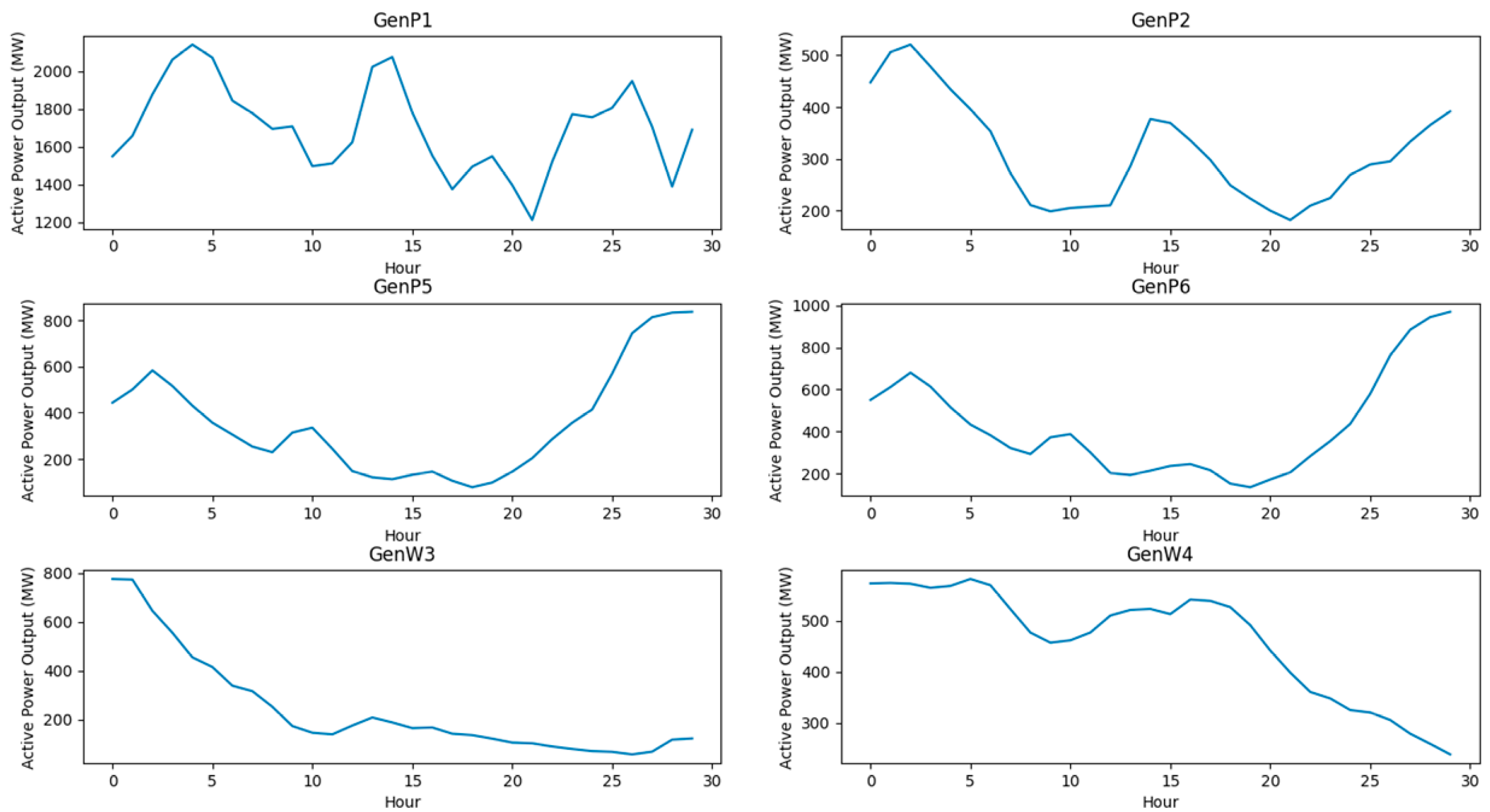
4.1.2. Wind Power Plant Output Curve

The output curve of a wind power plant is significantly influenced by weather conditions, particularly variations in wind speed and direction. Changes in wind speed directly affect the output power of the wind power plant, which can be described by the power curve. Generally, higher wind speeds result in higher output power, while lower wind speeds result in lower output power. Within a specific range of wind speeds (typically between the cut-in wind speed and the rated wind speed), the wind turbines can produce rated power. However, when the wind speed exceeds a certain limit (the cut-out wind speed), the wind turbines stop operating for protection, causing the output power to drop to zero. Under clear and cloudless conditions, wind speed is relatively stable, and the output power of the wind power plant fluctuates minimally. In cloudy and occasionally windy conditions, wind speed varies more, resulting in more significant fluctuations in output power. During storms or extreme weather conditions, wind speed fluctuates dramatically, leading to the highest fluctuations in output power and sometimes causing shutdowns if the cut-out wind speed is exceeded. This study uses a typical spring season as the verification scenario with a planning horizon of 240 h. The power generation data for a specific wind power plant are selected, and the output curves for the wind power plants on a certain day are shown in Figure 4 below. GenP1 corresponds to node 104, GenP2 to node 105, GenP5 to node 106, GenP6 to node 107, GenW3 to node 96, and GenW4 to node 97.

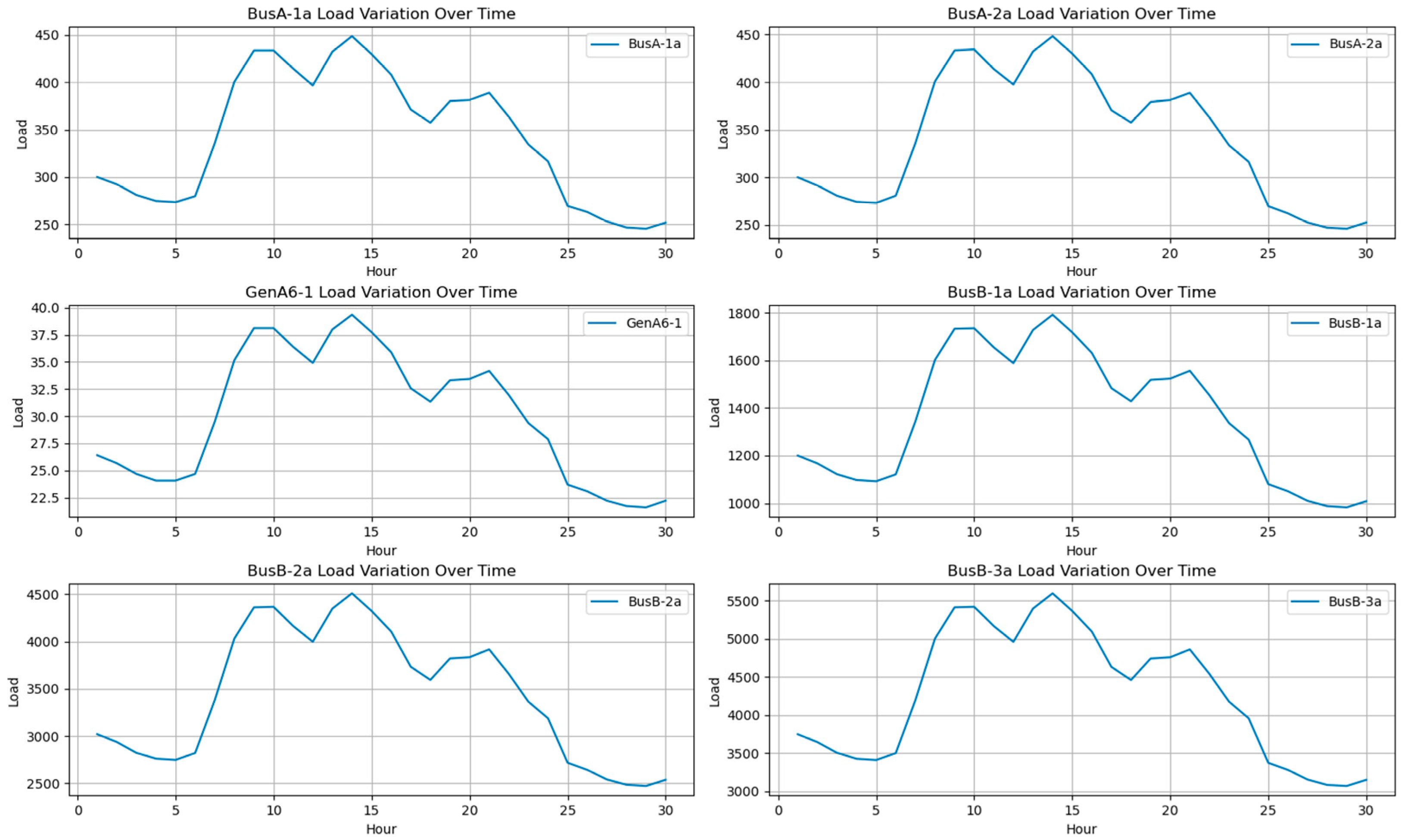
4.1.3. Grid Load Curve

The power system studied in this paper uses the same 240-h period as the wind power for the experimental scenario. The load fluctuation curve is shown in Figure 5. During the selected period, the grid load peaks around 10:00 AM and 3:00 PM and reaches its lowest point in the early morning. This pattern reflects a typical daily variation in power consumption.

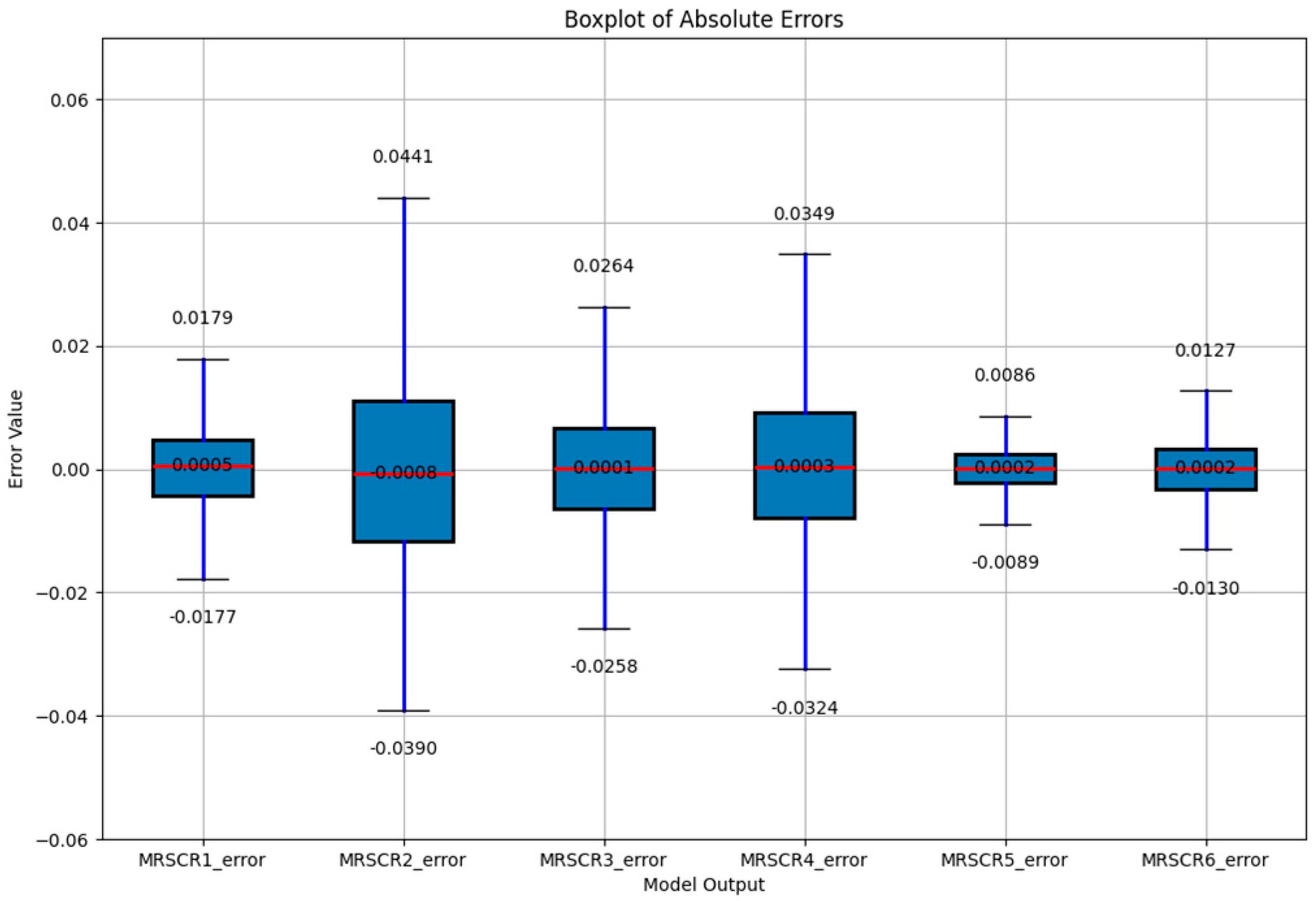
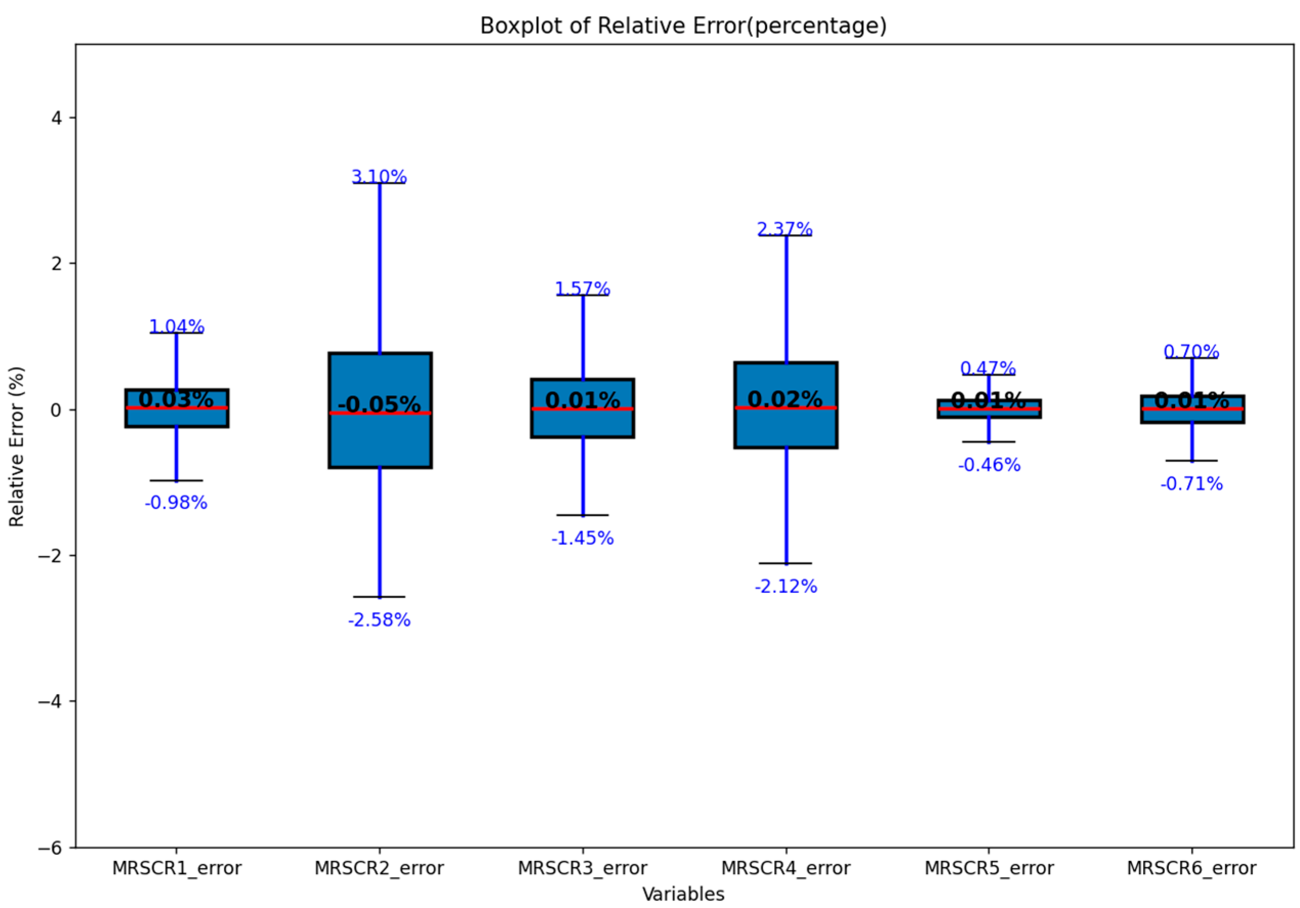
4.2. Fitting and Calculation of MRSCR Constraints

The power system used in the case study includes six wind farms, so i = 6i = 6i = 6. According to the methodology described in Section 2.3.2, the expression for the MRSCR for different wind farms is given by Equation (27).

$$MRSC{R}_1=2775.25/(P_1+0.1904P_2+0.1894P_3+0.1498P_4+0.1413P_5+0.1424P_6)$$

(29)

$$MRSC{R}_2=3568.05/(P_2+0.2094P_1+0.2546P_3+0.1902P_4+0.3184P_5+0.2436P_6)$$

(30)

$$MRSC{R}_3=2901.22/(P_3+0.1749P_1+0.1858P_2+0.1596P_4+0.1538P_5+0.1506P_6)$$

(31)

$$MRSC{R}_4=3592.84/(P_4+0.2206P_1+0.2299P_2+0.1013P_3+0.2616P_5+0.2422P_6)$$

(32)

$$MRSC{R}_5=2903.23/(P_5+0.1124P_1+0.1344P_2+0.1168P_3+0.0977P_4+0.1580P_6)$$

(33)

$${MRSCR}_6=2879.66/(P_6+0.1268P_1+0.1570P_2+0.1395P_3+0.1113P_4+0.1769P_5)$$

(34)

Based on the criterion of MRSCR > 1.5, we derived the constraints for the MRSCR. We randomly sampled 100 sets of data to fit Expressions (27) through (32) and another 1000 sets of data to calculate the formula results as the fitted values and compare them with the actual MRSCR values. The boxplot of the MRSCR fitting errors for the 6 wind farms is shown in the figure below.

As shown in Figure 6 and Figure 7, the fitting absolute errors range from approximately 0.01 to 0.04, with the maximum outlier deviating from the true value by 0.06. The maximum deviation of relative errors from the true value is 3.1%, indicating that the fitting results are relatively accurate. Thus, we can use the Gurobi solver to solve the model.

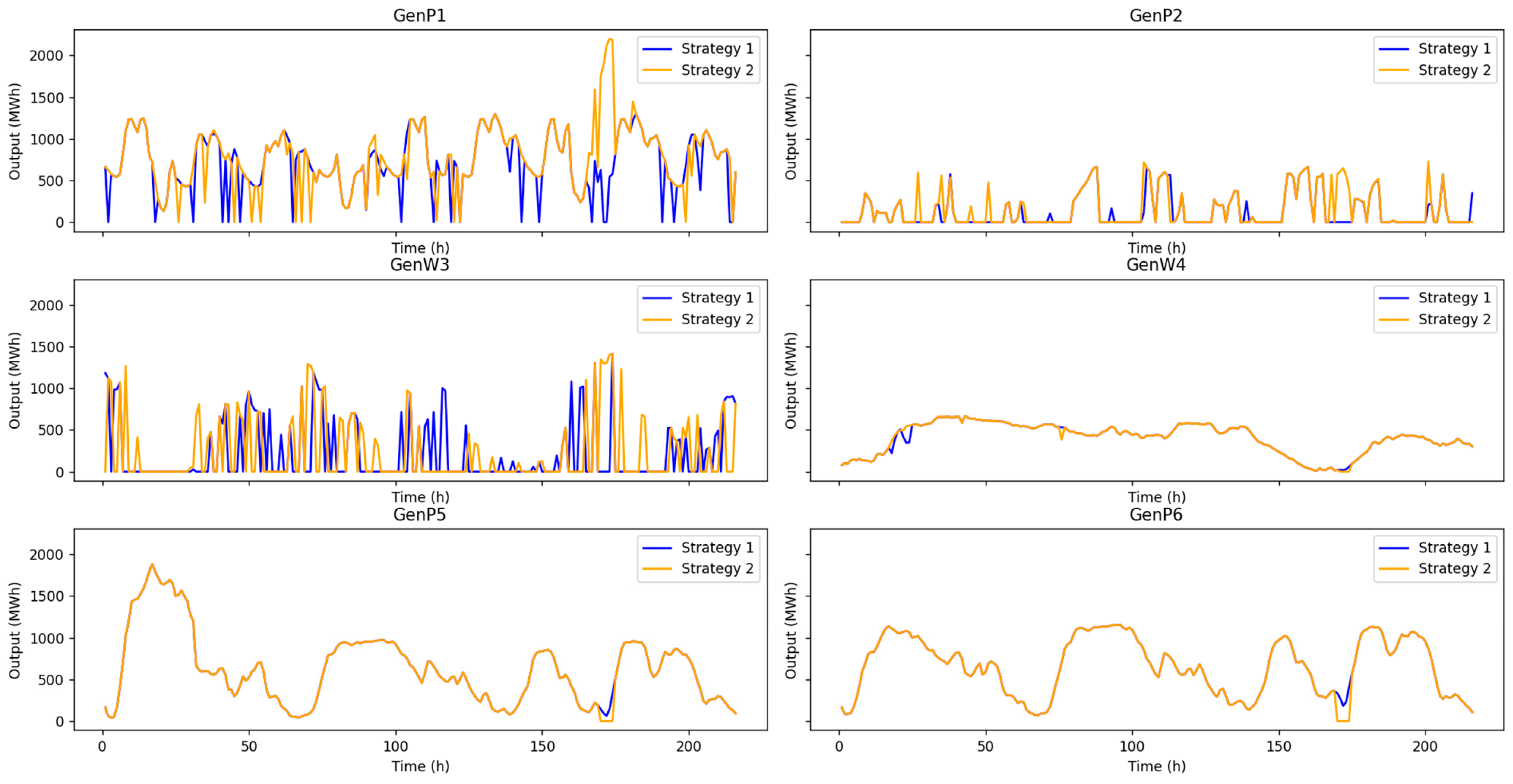
4.3. Experimental Results and Analysis

This case study compares the results of the model with MRSCR constraints to those without MRSCR constraints, highlighting the impact of MRSCR constraints on power system operation and scheduling.

Figure 8 shows the output of thermal and renewable energy units after solving the model. Wind (D) represents six wind power units connected at nodes 96, 97, 104, 105, 106, and 107. Thermal (A) represents thermal power units in Region A connected at nodes 78 to 87. Thermal (B) represents thermal power units in Region B connected at nodes 89 to 95. Thermal (C) represents thermal power units connected to the system balance node in Region C.

Figure 9 shows the output of thermal power units and wind farms after optimization, with and without considering MRSCR constraints.

In Figure 9, the blue curve (strategy 1) represents the scheduling results of wind farm outputs considering the MRSCR constraint, while the yellow curve (strategy 2) represents the scheduling results without considering the MRSCR constraint. The figure shows that the MRSCR constraint limits the output of each wind farm to some extent, reducing output fluctuations and improving wind power quality.

The power system dispatch results, considering whether the MRSCR constraint is applied, are shown in the following Figure 10:

In the figure, the black line represents the MRSCR of each wind farm with the MRSCR constraint, while the red line represents the MRSCR of each wind farm without the MRSCR constraint. It can be seen that the black line generally envelopes the red line, leaving a greater margin compared to the set standard of 1.5. The red line, on the other hand, falls below the standard of 1.5 in some cases where wind farm output is too high. This indicates that, in most cases, the MRSCR of each wind farm with the MRSCR constraint is better than that without the MRSCR constraint.

We extracted the MRSCR curves for each wind farm from the 165th to the 170th hour to illustrate the differences more clearly. Detailed information is shown in

Table 2. Comparison of MRSCR Results for Specific Periods at Different Stations.

TIME (h)	MRSCR1	MRSCR2	MRSCR3	MRSCR4	MRSCR5	MRSCR6
166	18.85373	18.31047	8.08322	13.35676	26.45281	6.22232
166	13.40469	12.00423	6.87182	10.07883	16.48418	3.26143
167	22.62489	30.29640	8.38348	14.65219	51.59498	43.5647
167	11.67327	11.33970	6.20249	8.689696	15.78557	3.29426
168	5.510105	2.191812	3.85195	4.620816	8.062710	2.82580
168	3.927695	1.767404	2.99019	3.282451	2.722518	1.45523
169	15.44229	14.38219	6.24638	9.245981	20.99923	5.19328
169	13.51455	12.22165	5.901937	8.432638	17.41708	3.92059
170	14.45075	13.29922	6.384079	9.916256	18.88385	4.16951
170	4.574496	1.817756	4.781466	4.385137	2.801712	1.38901

.

Similar to the figure, the black number represents strategy considered MRSCR constraint, the red number represents strategy neglect MRSCR constraint. MRSCR values below 1.5 are highlighted in yellow in the table. As shown in the table, the vertical coordinate of the black number is overall bigger: the smallest MRSCR at station1 of Strategy1 is 5.51, bigger than Strategy2’s 3.93; the smallest MRSCR at station2 of Strategy1 is 2.19, still bigger than Strategy2’s 1.77; the smallest MRSCR at station3 of Strategy1 is 3.85, bigger than Strategy2’s 2.99; the smallest MRSCR at Station 4 of Strategy1 is 4.62, bigger than Strategy2’s 3.28; the smallest MRSCR at Station 5 of Strategy1 is 8.06, bigger than Strategy2’s 2.72; and the smallest MRSCR at Station 6 of Strategy1 is 2.83. Meanwhile, Strategy2’s MRSCR has already dropped to the critical point of 1.5. At hour 170, the output of Wind Farm 6 without considering the MRSCR constraint reaches 1757.443 MW, with the MRSCR dropping to 1.39, below the standard of 1.5. However, the output of Wind Farm 6 considering the MRSCR constraint is reduced to 629.0049 MW, keeping the MRSCR above 3. The power deficit is compensated by thermal power units GenB1-1, GenB2-1, GenB2-2, and GenB2-3. An MRSCR value below the national standard of 1.5 will severely impact the integration of renewable energy into the grid, as a low MRSCR indicates insufficient voltage support capacity, leading to system oscillation and instability. The scheduling results considering the MRSCR constraint demonstrate superior performance in terms of this indicator.

The comparison table of scenarios considering and not considering the MRSCR constraint is shown in

Table 3. Comparison of Optimization Results for Different Scenarios.

Approach	Objective Function	Computation Time	Metric Evaluation
MRSCR-Constrained Approach	10,200,210.74	131.94 s	Better
MRSCR-Nonconstrained Approach	10,200,209.73	95.356 s	Normal

:

The results indicate that while the computation time for the scenario considering MRSCR constraints is longer, the economic benefits of the model are almost equivalent to those of the scenario without MRSCR constraints, significantly improving the stability of the MRSCR indicator.

5. Conclusions

This study investigates a power system active dispatch model constrained by MRSCR indicators. It simplifies the indicator approximation using the multivariate least squares and fits them into linear constraints closely related to the active output of renewable energy stations. The results indicate that the dispatch model, based on the MRSCR indicators, achieves optimal economic benefits and ensuring that the MRSCR exceeds 1.5 so that the system has an appropriate stability margin. This improves the system’s acceptance of renewable energy and reduces the fluctuations in renewable energy generation. To make the proposed method more suitable for real-world applications, several key points should be further addressed. Firstly, the assumptions used in the model are idealized and do not fully account for the complex factors in actual power grids, such as load fluctuations, equipment failures, and various uncertainties. Secondly, while the model performs well in terms of economic benefits and renewable energy integration, it lacks an in-depth analysis of environmental impacts and carbon emissions over long-term operations. In future research, we will conduct more detailed studies to address these limitations.

References

1. Zhou, X.; Lu, Z.; Liu, Y.; Chen, S. Development models and key technologies of future grid in China. Proc. CSEE 2014, 34, 4999–5008. (In Chinese) [Google Scholar]
2. Sun, H.; Xu, T.; Guo, Q.; Li, Y.; Lin, W.; Yi, J.; Li, W. Analysis on blackout in Great Britain power grid on August 9th, 2019 and its enlightenment to power grid in China. Proc. CSEE 2019, 39, 6183–6192. (In Chinese) [Google Scholar]
3. Ma, J.; Zhao, D.; Qian, M.; Zhu, L.; Yao, L.; Wang, N. Reviews of control technologies of large-scale renew-able energy connected to weakly-synchronized sending-end DC power grid. Power Syst. Technol. 2017, 41, 3112–3120. (In Chinese) [Google Scholar]
4. Kang, C.; Yao, L. Key scientific issues and theoretical research framework for power systems with high proportion of renewable energy. Autom. Electr. Power Syst. 2017, 41, 2–11. (In Chinese) [Google Scholar]
5. Sun, H.; Zhang, Z.; Lin, W.; Yang, Y.; Luo, X.; Wang, A. Analysis on serious wind turbine generators tripping accident in northwest China power grid in 2011 and its lessons. Power Syst. Technol. 2012, 36, 76–80. (In Chinese) [Google Scholar]
6. Ebrie, A.S.; Kim, Y.J. Reinforcement learning-based optimization for power scheduling in a renewable energy connected grid. Renew. Energy 2024, 230, 120886. [Google Scholar] [CrossRef]
7. Wu, Y.; Wang, C.; Wang, Y. Cooperative game optimization scheduling of multi-region integrated energy system based on ADMM algorithm. Energy 2024, 302, 131728. [Google Scholar] [CrossRef]
8. Zhu, X.; Hu, M.; Xue, J.; Li, Y.; Han, Z.; Gao, X.; Wang, Y.; Bao, L. Re-search on multi-time scale integrated energy scheduling optimization considering carbon constraints. Energy 2024, 302, 131776. [Google Scholar] [CrossRef]
9. Zhang, Y.; Ma, C.; Yang, Y.; Pang, X.; Liu, L.; Lian, J. Study on Short-Term Optimal Operation of Cascade Hydro-Photovoltaic Hybrid Systems. Appl. Energy 2021, 291, 116828. [Google Scholar] [CrossRef]
10. Guo, S.; Zheng, K.; He, Y.; Kurban, A. The Artificial Intelligence-Assisted Short-Term Optimal Scheduling of a Cascade Hydro Photovoltaic Complementary System with Hybrid Time Steps. Renew. Energy 2023, 202, 1169–1189. [Google Scholar] [CrossRef]
11. Aguilar, D.; Quinones, J.J.; Pineda, L.R.; Ostanek, J.; Castillo, L. Optimal sched-uling of renewable energy microgrids: A robust multi-objective approach with machine learning-based probabilistic forecasting. Appl. Energy 2024, 369, 123548. [Google Scholar] [CrossRef]
12. Gao, Y.; Chang, X.; Xue, Y.; Su, J.; Li, Z.; Sun, H. Interval Optimization Scheduling of Renewable Hydrogen Refueling Stations Considering Wind and Solar Uncertainties and Dynamic Hydrogen Prices. Power Syst. Technol. 2024, 1–13. [Google Scholar] [CrossRef]
13. Dong, Z.; Zhang, Z.; Huang, M.; Yang, S.; Zhu, J.; Zhang, M.; Chen, D. Research on day-ahead optimal dispatching of virtual power plants considering the coordinated operation of diverse flexible loads and new energy. Energy 2024, 297, 131235. [Google Scholar] [CrossRef]
14. Li, X.; Dong, Y.; Liu, H.; Yao, Z. Multi-Time-Scale Scheduling Model for Renewable Energy Grid Integration Considering the Generalized Short-Circuit Ratio. Mod. Electr. Power 2024, 41, 240–248. (In Chinese) [Google Scholar] [CrossRef]
15. Vineeth, V.V.; Vijayalakshmi, V.J. A novel deep learning approach for estimating and classifying short-term voltage stability events in modern power systems with composite load and distributed energy resources. Electr. Eng. 2024, 1–13. [Google Scholar] [CrossRef]
16. Paul, C.; Sarkar, T.; Dutta, S.; Hazra, S.; Roy, P.K. Optimal Power Flow of Multi-objective Combined Heat and Power with Wind-Solar-Electric Vehicle-Tidal Using Hybrid Evolutionary Approach. Process Integr. Optim. Sustain. 2024, 1–31. [Google Scholar] [CrossRef]
17. Hong, H. Optimization Scheduling of Novel Power Systems Considering Frequency-Inertia Safety Constraints; Hangzhou Dianzi University: Hangzhou, China, 2024. (In Chinese) [Google Scholar] [CrossRef]
18. Zhang, Y. Study on the Impact of UPFC and New Energy Devices on Power System Stability; North China Electric Power University: Beijing, China, 2017. (In Chinese) [Google Scholar]
19. Lai, B. Optimization Operation and Small Disturbance Stability Analysis of New Energy Power Systems; North China Electric Power University: Beijing, China, 2016. (In Chinese) [Google Scholar]
20. Jia, H.; Wang, L. Study on Small Disturbance Stability of Power Systems with Large-Scale Wind Farms. Power Syst. Technol. 2012, 36, 61–69. (In Chinese) [Google Scholar] [CrossRef]
21. Zhang, H.; Zhang, L.; Chen, S.; An, N. Impact of Large-Scale Wind Farms on the Small Disturbance Stability and Damping Characteristics of Power Systems. Power Syst. Technol. 2007, 13, 75–80. (In Chinese) [Google Scholar]
22. GB 38755-2019; Code on Security and Stability for Power System. National Energy Agency: Beijing, China, 2019.
23. Zhang, Y.; Huang, S.H.; Schmall, J.; Conto, J.; Billo, J.; Rehman, E. Evaluating system strength for large-scale wind plant integration. In Proceedings of the IEEE PES General Meeting, National Harbor, MD, USA, 27–31 July 2014. [Google Scholar]
24. Report to NERC ERSTF for Composite Short Circuit Ratio (CSCR) Estimation Guideline; GE Energy Consulting: Sche-nectady, NY, USA, 2015.
25. CIGRE. CIGRE Working Group B4.41. In Connection of Wind Farms to Weak AC Networks; CIGRE: Paris, France, 2016. [Google Scholar]
26. Wu, D.; Li, G.; Javadi, M.; Malyscheff, A.M.; Hong, M.; Jiang, J.N. Assessing impact of renewable energy integration on system strength using site-dependent short circuit ratio. IEEE Trans. Sustain. Energy 2018, 9, 1072–1080. [Google Scholar] [CrossRef]
27. Sun, H.; Xu, S.; Xu, T.; Guo, Q.; He, J.; Zhao, B.; Yu, L.; Zhang, Y.; Li, W.; Zhou, Y. Definition and Metrics of Multiple Renewable Energy Station Short-Circuit Ratio. Proc. CSEE 2021, 41, 497–506. (In Chinese) [Google Scholar] [CrossRef]
Figure 1. Simplified model of AC system connected with multiple renewable energy stations.
Electronics 13 03811 g001
Figure 2. Flowchart of Multivariate Least Squares Fitting for MRSCR Constraints.
Electronics 13 03811 g002
Figure 3. Network Topology of the 109-Node Power System.
Electronics 13 03811 g003
Figure 4. Output Curves of Different Wind Power Plants.
Electronics 13 03811 g004
Figure 5. Grid Load Curve.
Electronics 13 03811 g005
Figure 6. Boxplot of Absolute Errors in MRSCR Fitting.
Electronics 13 03811 g006
Figure 7. Boxplot of Relative Errors in MRSCR Fitting (percentage).
Electronics 13 03811 g007
Figure 8. Stacked percentage output over time for wind and thermal generators.
Electronics 13 03811 g008
Figure 9. Power Output Planning Curves for Wind Farms with and without MRSCR Constraints.
Electronics 13 03811 g009
Figure 10. Comparison of MRSCR Results.
Electronics 13 03811 g010