High-Precision Forward Modeling of Controlled Source Electromagnetic Method Based on Weighted Average Extrapolation Method

Abstract

To achieve high-precision calculation of the electromagnetic field of layered media and to ensure that the apparent resistivity calculation and sensitivity are not affected by numerical errors, this paper implements high-precision calculation of the layered electromagnetic field based on the weighted average (WA) extrapolation method. Firstly, the 1D electromagnetic field expression of an arbitrary attitude field source is obtained by using the magnetic vector potential; then, the WA extrapolation technique is introduced to achieve the high-precision and fast solution of the Hankel transform, and the effects of the number of Gaussian points and the number of integration intervals on the accuracy are investigated. The theoretical model test shows that, compared with the open-source Dipole1D, the algorithm proposed in this paper has wider adaptability, and can achieve high-precision calculation of electric and magnetic dipole sources with higher efficiency. Compared with the epsilon algorithm studied by previous researchers, the WA extrapolation method proposed in this article can improve the convergence rate by approximately 20% under the same conditions. It can obtain high-precision numerical solutions with less integration time. The relative accuracy can reach the order ${10}^{-10}$, and its computational efficiency is significantly better than the existing epsilon algorithm. Finally, we used two cases of marine controlled source electromagnetic method to show the application. The sensitivity and Poynting vectors are calculated, which provides a technical tool for a deep understanding of physical mechanisms in layered media.

1. Introduction

There are many variations of the basic electromagnetic sounding technique, and it is necessary to have an in-depth understanding of the mathematical and physical characteristics of the field sources. An understanding of the basic theory of electromagnetic fields is useful in determining the similarities, capabilities and limitations of electromagnetic sounding techniques for different sources. The knowledge of the basic distribution and composition of fields under layered media is fundamental to the theory of electromagnetic detection. The methods for deriving EM fields under layered media can be divided into two categories, one directly adopts EM field components [1,2,3]. The other employs potential field, such as using the Hertiz potential [4], the Schelkunoff potential [5], and vector potential [6,7]. Directly using the electromagnetic field derivation is more complicated, and not conducive to understanding the components of the field, in this paper, with the help of vector potential based on the Lorentz gauge for the derivation, the derivation of the formulae under the layered medium considering the magnetic permeability and electrical conductivity [8]. We first derive the expressions for the field components of the horizontal and vertical electric dipole sources; however, the duality is used to obtain the response of the horizontal and vertical magnetic dipole sources by interchanging the electric and magnetic permeability parameters.

Mosig [9] pointed out that Sommerfeld integrals can provide direct evaluations of the involved electromagnetic fields. Disciplines involving layered media, like seismology and geological prospection, also benefit from these integrals in the geophysical EM method. The formulas for both the horizontal and vertical dipole sources are finally transformed into a numerical integration of the product of the kernel function and the Bessel function over the interval from zero to infinity, i.e., the Hankel transform. The Bessel function decays slowly and oscillates violently, making the calculation of Hankel transform difficult. Commonly used methods include digital filtering methods, extrapolated accelerated numerical integration methods, and complex mirror image methods. Filtering algorithms are the most commonly used methods in geophysics and have the advantage of fast computation speed, which can be achieved using lagged convolution for fast computation at multiple measurement points, and the method is widely used in geophysics [10].

Numerical integration methods have the advantage of controllable accuracy. Hunziker [3] used a 61-point Gauss–Kronrod integral to implement calculations of the Hankel transform, with the upper limit of the integral typically being twice the Nyquist frequency of the spatial sampling rate. He computed the Hankel transform at a portion of the measurement points in the spatial domain, and then obtained the field values of the other measurement points by cubic spline interpolation to obtain the field values at other measurement points. He also pointed out that the field value accuracy can be greatly improved by increasing the number of numerical integration points, but the computational efficiency is relatively low. To improve the computational efficiency of numerical integration, extrapolation acceleration methods have been proposed, such as Euler transform, Levin-type transforms, robust epsilon algorithm [11] (i.e., shanks transform of sequences), and Weighted Averages (WA) extrapolation method. Weniger [12] gave a review of the level acceleration methods and nonlinear transformation methods. Lucas and Stone [13] illustrated the selection of breakpoints and pointed out that the consecutive zeros of the Bessel function were the best choices of breakpoints. Michalski [14] systematically deduced and compared different extrapolation methods, and introduced several extrapolation algorithms best suited for the integration of Sommerfeld tails. Their performances are also compared, and it is pointed out that the WA method and the W-algorithm in Levin-type transforms are usually the most versatile and effective convergence accelerators for integration formulas in multilayer media.

Sequence and extrapolation acceleration have been less used in geophysics. Chave [4] used the concatenated fractional method to accelerate the convergence of integral tails for one-dimensional computation of electromagnetic fields in geophysics. Key [11] studied the epsilon algorithmic extrapolation and compared the accuracy and efficiency with that of digital filtering algorithms, and found that the algorithm converged faster, stably, and with controllable accuracy.

As a technique to compute the tails of Sommerfeld integrals appearing in Green’s function formulation of planar multilayer problems, the WA algorithm was introduced in the microwave and antenna fields [7,9]. Michalski further extended and improved the WA algorithm in his review paper [14]. Mosig [9,15] reviewed and reevaluated the classical WA algorithm and introduced a new implementation of the WA algorithm. Golubović et al. [16] applied the method to the integral function of the Bessel function and the results showed that it can still converge quickly. The algorithm can even be efficiently applied to anomalous integrals including oscillatory or divergent product functions. The WA method is one of the most efficient extrapolation methods applied to accelerate the convergence of integral sequences. Lovat [17] compared the most powerful extrapolation techniques, i.e., the Levin–Sidi extrapolation method and the generalized weighted averages method. Extensive numerical results clearly show the robustness, the accuracy, and the efficiency of the proposed method: in particular, for a class of integrals often encountered in a variety of applications. Therefore, it has been widely used in the field of computational electromagnetism.

However, sequence and extrapolation acceleration have been less used in geophysics. As a classic quadrature with extrapolation method, the epsilon algorithm has been widely adopted. Key [11] studied the epsilon algorithmic extrapolation and compared the accuracy and efficiency with that of digital filtering algorithms, and found that the algorithm converged faster, stably, and with controllable accuracy. Liu [8] adapted the epsilon algorithm to calculate the integration of Bessel functions to produce EM responses with the desired accuracy. Kien [18] presents a C++ package using quadrature with extrapolation (the epsilon algorithm) which computes the electromagnetic field for a one-dimensional model in geophysics.

The WA algorithm, which is commonly used and considered to be one of the best algorithms in computational electromagnetism, has not been studied in geophysical electromagnetic methods. This paper introduces the algorithm into the field of geophysical electromagnetic methods and studies the efficiency and accuracy of the algorithm. To achieve high accuracy and ensure that the apparent resistivity calculations and sensitivity are not affected by numerical errors, this paper implements a new extrapolation method, i.e., the classical Mosig–Michalski version of the weighted extrapolation algorithm [19], and investigates the numerical accuracy of the method concerning the number of Gaussian points, the number of integration interval segment relationships, and the reliability of the algorithm for calculating sensitivity and energy flow density is verified.

2. Methods

The basic procedure for the derivation of the electromagnetic field of a layered medium is as follows: firstly, the potential field of each layer is expressed as the sum of the general solution and the special solution, the special solution is the expression of the potential field of the source in the homogeneous full space, and the general solution of each layer is controlled by the interlayer coefficients [7]. Then, the recurrence relation of the interlayer coefficients is obtained by using the layer interface junction condition to form a system of equations for the interlayer coefficients. With the help of reflection coefficients, the general coefficients of the field source layer are solved first, and then the general coefficients of each layer are obtained by the recursive equation, to obtain the electromagnetic field at any position. In this paper, the derivation is extended to the magnetic dipole source, and the permeability variation is considered; the expressions for the field components of the horizontal and vertical electric dipole sources are obtained first; however, the response of the horizontal and vertical magnetic dipole sources is obtained by interchanging the electric and magnetic permeability parameters using the duality.

2.1. Layered Medium Response Expression

This section derives expressions for the fields generated by a source at any location. Establish a right-handed coordinate system with the z-axis facing down, see Figure 1, where the electric field $E$ and the magnetic field $B$ can be expressed in magnetic vector potential $A$ (See Equation (5) for details). The field can be specified as:

$$\begin{array}{l}E=i\omega A+\nabla \left({\displaystyle \frac{\nabla ·A}{\mu \sigma }}\right)\\ B=\nabla \times A\end{array}$$

(1)

At the interface, the electric and magnetic fields satisfy the tangential continuity boundary condition:

$$\begin{array}{l}{E}_{x1}=E_{x2},E_{y1}=E_{y2}\\ H_{x1}=H_{x2}, H_{y1}=H_{y2}\end{array}$$

(2)

Substituting Equation (1) into the boundary condition Equation (2) yields an articulation condition concerning the vector potential at the layer interface.

2.1.1. Horizontal Dipole Sources

Assume that the horizontal electric dipole source is along the y-direction, the source is located in the jth layer, the electric conductivity of each layer is $\left({\sigma }_1,{\sigma }_2,\cdots {\sigma }_n\right)$, the magnetic permeability is $\left({\mu }_1,{\mu }_2,\cdots {\mu }_n\right)$, and for a land source, ${\sigma }_1$ is the air layer, $I$ is transmission current. In each layer, substituting the vector potential into the electromagnetic field dual curl equation with moments $Ids{u}_{\mathrm{y}}$, electric dipole $J_e^s=u_{y}I\delta (x)\delta (y)\delta (z)$, yields vector potential $A$ satisfying the equation.

$${\nabla }^2{A}_i+i\omega \mu {\sigma }_i{A}_i=-\mu J_s$$

(3)

To facilitate the solution, Equation (3) is 2D Fourier transformed in the x and y directions and converted to the Hankel transform, and the control equation becomes:

$$\begin{array}{c}-{\displaystyle \frac{{\partial }^2{\widehat{\mathrm{A}}}_{y\mathrm{i}}}{\partial z^2}}+{\gamma }_i^2{\widehat{A}}_{yi}=\mu {\widehat{J}}_{yi}\hspace{0.33em}\hspace{0.33em}\hspace{0.33em}\hspace{0.33em}\hspace{0.33em}\hspace{0.33em}\hspace{0.33em}\hspace{0.33em}\hspace{0.33em}\hspace{0.33em}\hspace{0.33em}\hspace{0.33em}\hspace{0.33em}\hspace{0.33em}\hspace{0.33em}\hspace{0.33em}\hspace{0.33em}\hspace{0.33em}\hspace{0.33em}\hspace{0.33em}\hspace{0.33em}\hspace{0.33em}\hspace{0.33em}i=1,\cdots ,n\\ -{\displaystyle \frac{{\partial }^2{\widehat{\mathsf{\Lambda }}}_{zi}}{\partial z^2}}+{\gamma }_i^2{\widehat{\mathsf{\Lambda }}}_{zi}=0\hspace{0.33em}\hspace{0.33em}\hspace{0.33em}\hspace{0.33em}\hspace{0.33em}\hspace{0.33em}\hspace{0.33em}\hspace{0.33em}\hspace{0.33em}\hspace{0.33em}\hspace{0.33em}\hspace{0.33em}\hspace{0.33em}\hspace{0.33em}\hspace{0.33em}\hspace{0.33em}\hspace{0.33em}\hspace{0.33em}\hspace{0.33em}\hspace{0.33em}\hspace{0.33em}\hspace{0.33em}\hspace{0.33em}\hspace{0.33em}\hspace{0.33em}\hspace{0.33em}i=1,\cdots ,n\end{array}$$

(4)

where the following relationship exists between the wavenumber domain ${\widehat{\mathrm{A}}}_{y\mathrm{i}}$ and the spatial domain $A_y$, the wavenumber domain ${\widehat{\mathsf{\Lambda }}}_z$ and the spatial domain $A_z$:

$$\begin{array}{l}{A}_y\left(r\right)={\displaystyle \frac{1}{2\pi }}{\displaystyle {\int }_0^{\infty }{\widehat{A}}_y\left(\lambda ,z\right)}{J}_0\left(\lambda r\right)\lambda d\lambda \\ A_z\left(r\right)={\displaystyle \frac{1}{2\pi }}{\displaystyle \frac{\partial }{\partial y}}{\displaystyle {\int }_0^{\infty }{\widehat{\mathsf{\Lambda }}}_z\left(\lambda ,z\right)}{J}_0\left(\lambda r\right)\lambda d\lambda \end{array}$$

(5)

It is necessary to solve for the wavenumber domain ${\widehat{A}}_y\left(\lambda ,z\right),{\widehat{\mathsf{\Lambda }}}_z\left(\lambda ,z\right)$, and then the magnetic vector potential in the space domain can be obtained by using Equation (5). For the y-direction electric dipole source $J_e^s=u_{y}I\delta (x)\delta (y)\delta (z)$, the magnetic vector potential in the space domain should be represented by two components $A=\left(0,A_y,A_z\right)$, so that $A_z=\partial {\mathsf{\Lambda }}_z/\partial y$, borrowed from Λ_z, can simplify the subsequent derivation, and in the wavenumber domain ${\widehat{A}}_z=i{k}_y{\widehat{\mathsf{\Lambda }}}_z$. In the following text, if not otherwise specified, the variable $\widehat{A}$ indicates that it is in the wavenumber domain, and the variable $A$ indicates that it is in the space domain.

The special solution together with the corresponding general solution table yields a representation of the wavenumber domain vector potential in the $z\in \left[z_i,z_{i+1}\right]$ layer [20]:

$$\begin{array}{l}{\widehat{A}}_{yi}=a_i{e}^{{\gamma }_i\left(z-z_{i+1}\right)}+b_i{e}^{-{\gamma }_i\left(z-z_i\right)}+{\delta }_{ij}{\displaystyle \frac{{\mu }_j}{2{\gamma }_j}}{e}^{-{\gamma }_j|z-z_s|}\\ {\lambda }^2{\widehat{\mathsf{\Lambda }}}_{zi}={\mu }_i\left[c_i{e}^{{\gamma }_i\left(z-z_{i+1}\right)}+d_i{e}^{-{\gamma }_i\left(z-z_i\right)}\right]-{\gamma }_i\left[a_i{e}^{{\gamma }_i\left(z-z_{i+1}\right)}-\hspace{0.33em}{b}_i{e}^{-{\gamma }_i\left(z-z_i\right)}\right]\end{array}$$

(6)

where $z_i$ denotes the depth of the top layer $i$, $z_s$ denotes the depth of the field source, $j$ denotes the layer in which the source is located, and ${\delta }_{ij}$ denotes the source distribution function, which is ${\delta }_{ij}=1$ if $j=i$ and zero otherwise. The coefficients $b_1,d_1,c_n,a_n$ are all zero because the electromagnetic field decays to zero at z infinity.

To solve for the coefficients of each layer and to determine the ${\widehat{A}}_{\mathrm{i}}$ of each layer, it is necessary to analyze the recurrence relation between ${\widehat{A}}_{\mathrm{i}}$ and ${\widehat{A}}_{\mathrm{i}-1}$. Substituting the wavenumber domain magnetic vector potential into the continuity conditions for the electric and magnetic field Equation (2) yields the boundary conditions for the wavenumber domain magnetic vector potential:

$$\begin{array}{c}{\displaystyle \frac{1}{{\mu }_{\mathrm{i}}{\sigma }_i}}\left({\widehat{A}}_{yi}+{\displaystyle \frac{\partial {\widehat{\mathsf{\Lambda }}}_{zi}}{\partial z}}\right)={\displaystyle \frac{1}{{\mu }_{i+1}{\sigma }_{i+1}}}\left({\widehat{A}}_{yi+1}+{\displaystyle \frac{\partial {\widehat{\mathsf{\Lambda }}}_{zi+1}}{\partial z}}\right)\\ {\widehat{A}}_{yi}={\widehat{A}}_{yi+1}\\ {\displaystyle \frac{1}{{\mu }_i}}{\displaystyle \frac{\partial {\widehat{A}}_{yi}}{\partial z}}={\displaystyle \frac{1}{{\mu }_{i+1}}}{\displaystyle \frac{\partial {\widehat{A}}_{yi+1}}{\partial z}}\\ {\displaystyle \frac{1}{{\mu }_i}}{\widehat{\mathsf{\Lambda }}}_{zi}={\displaystyle \frac{1}{{\mu }_{i+1}}}{\widehat{\mathsf{\Lambda }}}_{zi+1}\end{array}$$

(7)

where ${\gamma }_i=\sqrt{{\lambda }^2-i\omega {\mu }_i{\sigma }_i}$. Substituting the expression of each layer’s potential field Equation (6) into the boundary conditions of Equation (7) yields a system of $4n-4$ equations relating the generalized solution coefficients of each layer, together with the known $b_1=d_1=c_n=a_n=0$, forming 4n equations.

If the coefficients are obtained by directly solving the inverse of the formed system of equations, there will be numerical instability. The solution can be carried out recursively layer by layer, and there are two ways of linking layer-to-layer coefficients. One is the layer-by-layer coefficient recursion used in this paper; the other is the matrix-propagation technique. The use of matrix-propagation techniques is prone to the presence of positive exponential terms, leading to numerical stability problems. Special treatment is required when dealing with the layer where the field source is located to deal with the junction conditions, which need to be divided into the upper and lower source layer interfaces for separate derivations.

For the source layer upper interface $\left(i=j\right)$:

$$\begin{array}{l}{a}_j{e}^{-{\gamma }_j{l}_j}+b_j+{\displaystyle \frac{{\mu }_j}{2{\gamma }_j}}{e}^{-{\gamma }_j|z_j-z_s|}=a_{j-1}+b_{j-1}{e}^{-{\gamma }_{j-1}{l}_{j-1}}\\ {\displaystyle \frac{1}{{\mu }_j}}\left(a_j{\gamma }_j{e}^{-{\gamma }_j{l}_j}-b_j{\gamma }_j-{\displaystyle \frac{{\mu }_j\mathrm{sgn}|z_j-z_s|}{2}}{e}^{-{\gamma }_j|z_j-z_s|}\right)={\displaystyle \frac{1}{{\mu }_{j-1}}}\left(a_{j-1}{\gamma }_{j-1}-b_{j-1}{\gamma }_{j-1}{e}^{-{\gamma }_{j-1}{l}_{j-1}}\right)\\ \left(c_j{e}^{-{\gamma }_j{l}_j}+d_j\right)-{\displaystyle \frac{\mathrm{sgn}(z_j-z_s)}{2}}{e}^{-{\gamma }_j\left|z_j-zs\right|}=\left(c_{j-1}+d_{j-1}{e}^{-{\gamma }_{j-1}{l}_{j-1}}\right)\\ {\displaystyle \frac{1}{{\sigma }_j}}\left(\left[\left({\gamma }_j{c}_j{e}^{-{\gamma }_j{l}_j}-{\gamma }_j{d}_j\right)+{\displaystyle \frac{1}{2}}\left({\gamma }_j{e}^{-{\gamma }_j\left|z_j-z_s\right|}\right)\right]\right)={\displaystyle \frac{1}{{\sigma }_{j-1}}}\left(\left[\left({\gamma }_{j-1}{c}_{j-1}-{\gamma }_{j-1}{d}_{j-1}{e}^{-{\gamma }_{j-1}{l}_{j-1}}\right)\right]\right)\end{array}$$

(8)

For the source layer lower interface $\left(i=j+1\right)$, the simplified expression is:

$$\begin{array}{l}{a}_{j+1}{e}^{-{\gamma }_{j+1}{l}_{j+1}}+b_{j+1}=a_j+b_j{e}^{-{\gamma }_j{l}_j}+{\displaystyle \frac{{\mu }_j}{2{\gamma }_j}}{e}^{-{\gamma }_j|z_{j+1}-z_s|}\\ {\displaystyle \frac{1}{{\mu }_{j+1}}}\left(a_{j+1}{\gamma }_{j+1}{e}^{-{\gamma }_{hj+1}{l}_{j+1}}-b_{j+1}{\gamma }_{j+1}\right)={\displaystyle \frac{1}{{\mu }_j}}\left(a_j{\gamma }_j-b_j{\gamma }_j{e}^{-{\gamma }_j{l}_j}-{\displaystyle \frac{{\mu }_j\mathrm{sgn}\left|z_{j+1}-z_s\right|}{2}}{e}^{-{\gamma }_j|z_{j+1}-z_s|}\right)\\ \left(c_{j+1}{e}^{-{\gamma }_{j+1}{l}_{j+1}}+d_{j+1}\right)=\left(c_j+d_j{e}^{-{\gamma }_j{l}_j}\right)-{\displaystyle \frac{\mathrm{sgn}(z_{j+1}-z_s)}{2}}\left(e^{-{\gamma }_j\left|z_{j+1}-z_s\right|}\right)\\ {\displaystyle \frac{1}{{\sigma }_{j+1}}}\left(\left[\left({\gamma }_{j+1}{c}_{j+1}{e}^{-{\gamma }_{j+1}{l}_{j+1}}-{\gamma }_{j+1}{d}_{j+1}\right)\right]\right)={\displaystyle \frac{1}{{\sigma }_j}}\left(\left[\left({\gamma }_j{c}_j-{\gamma }_j{d}_j{e}^{-{\gamma }_j{l}_j}\right)+{\displaystyle \frac{1}{2}}\left({\gamma }_j{e}^{-{\gamma }_j\left|z_{j+1}-zs\right|}\right)\right]\right)\end{array}$$

(9)

Equations (8) and (9) form 4n equations, and it can be shown that $a_{i,}{b}_i$$c_{i,}{d}_i$ and are completely decoupled and can be solved independently.

The global reflection coefficients $R_i^{-},R_i^{+},S_i^{+},S_i^{-}$ and local reflection coefficients $r_i^{-},r_i^{+},s_i^{-},s_i^{+}$ are derived for all layers, where $R_i^{-},S_i^{-},r_i^{-},s_i^{-}$ exist only in the source and upper source layers, recursively from layer 1 to layer $j$, and $R_i^{+},S_i^{+},r_i^{+},s_i^{+}$ exist only in the source and lower source layers, recursively from the bottom layer to layer $j$. After obtaining all the coefficients of the source layer, the remaining layers are obtained by recursion from the source layer. From the interlayer coefficients, the magnetic vector potential is obtained and converted to the electromagnetic field components using Equation (1). The final expression for the electromagnetic field components can be obtained as:

$$\begin{array}{l}{E}_x=-{\displaystyle \frac{\sin 2\phi }{4\pi \mu {\sigma }_i}}{\displaystyle {\int }_0^{\infty }({\widehat{\mathrm{A}}}_y(\lambda ,z)+\frac{\partial {\widehat{\mathsf{\Lambda }}}_z(\lambda ,z)}{\partial z}})({\lambda }^3{J}_0(\lambda r)-{\displaystyle \frac{2{\lambda }^2}{r}}{J}_1(\lambda r))d\lambda \\ E_y={\displaystyle \frac{i\omega }{2\pi }}{\displaystyle {\int }_0^{\infty }{\widehat{\mathrm{A}}}_y(\lambda ,z)\lambda J_0(\lambda r)d\lambda }-{\displaystyle \frac{{\cos }^2\phi }{2\pi \mu {\sigma }_i}}{\displaystyle {\int }_0^{\infty }({\widehat{\mathrm{A}}}_y(\lambda ,z)+\frac{\partial {\widehat{\mathsf{\Lambda }}}_z(\lambda ,z)}{\partial z}}){\lambda }^3{J}_0(\lambda r)d\lambda \\ \hspace{0.33em}\hspace{0.33em}\hspace{0.33em}\hspace{0.33em}\hspace{0.33em}\hspace{0.33em}\hspace{0.33em}+{\displaystyle \frac{\cos 2\phi }{2\pi \mu {\sigma }_i}}{\displaystyle {\int }_0^{\infty }({\widehat{\mathrm{A}}}_y(\lambda ,z)+\frac{\partial {\widehat{\mathsf{\Lambda }}}_z(\lambda ,z)}{\partial z}}){\displaystyle \frac{{\lambda }^2}{r}}{J}_1(\lambda r)d\lambda \\ E_z=-{\displaystyle \frac{\cos \phi }{2\pi \mu {\sigma }_i}}{\displaystyle {\int }_0^{\infty }({\lambda }^2{\widehat{\mathsf{\Lambda }}}_z(\lambda ,z)+\frac{\partial {\widehat{\mathrm{A}}}_y(\lambda ,z)}{\partial z}}){\lambda }^2{J}_1(\lambda r)d\lambda \\ H_x=-{\displaystyle \frac{\cos 2\phi }{4\pi {\mu }_i}}\left[{\displaystyle {\int }_0^{\infty }{\widehat{\mathsf{\Lambda }}}_z(\lambda ,z)({\lambda }^3{J}_0(\lambda r)-\frac{2{\lambda }^2}{r}{J}_1(\lambda r))}d\lambda \right]\\ \hspace{0.33em}\hspace{0.33em}\hspace{0.33em}\hspace{0.33em}\hspace{0.33em}\hspace{0.33em}\hspace{0.33em}-{\displaystyle \frac{1}{2\pi {\mu }_i}}\left[{\displaystyle {\int }_0^{\infty }\left(\frac{1}{2}{\lambda }^2{\widehat{\mathsf{\Lambda }}}_z(\lambda ,z)+\frac{\partial {\widehat{\mathrm{A}}}_y(\lambda ,z)}{\partial z}\right)\lambda J_0(\lambda r)}d\lambda \right]\\ H_y={\displaystyle \frac{\sin 2\phi }{4\pi {\mu }_i}}{\displaystyle {\int }_0^{\infty }({\widehat{\mathsf{\Lambda }}}_z(\lambda ,z)})({\lambda }^3{J}_0(\lambda r)-{\displaystyle \frac{2{\lambda }^2}{r}}{J}_1(\lambda r))d\lambda \\ H_z=-{\displaystyle \frac{\sin \phi }{2\pi {\mu }_i}}{\displaystyle {\int }_0^{\infty }({\widehat{\mathrm{A}}}_y(\lambda ,z)}){\lambda }^2{J}_1(\lambda r)d\lambda \end{array}$$

(10)

In the above equation $\sin \phi =x/r$, all electromagnetic field components are expressed in the form of the Hankel transform.

2.1.2. Vertical Electric Dipole Source

For the z-direction electric dipole $J_e^s=u_{z}I\delta (x)\delta (y)\delta (z-z_s)$, the magnetic vector is simple $A_z$. For the ith layer, Equation (3) transforms to:

$${\displaystyle \frac{{\partial }^2{\widehat{A}}_z}{\partial z^2}}-{\gamma }_i^2{\widehat{A}}_z=-\mu J_s$$

(11)

Substituting to the continuous boundary, the boundary conditions that should be satisfied are:

$$\begin{array}{l}{\displaystyle \frac{1}{{\mu }_1}}{\widehat{A}}_{z1}={\displaystyle \frac{1}{{\mu }_2}}{\widehat{A}}_{z2}\\ {\displaystyle \frac{1}{{\mu }_1{\sigma }_1}}{\displaystyle \frac{{\widehat{\partial A}}_{z1}}{\partial z}}={\displaystyle \frac{1}{{\mu }_2{\sigma }_2}}{\displaystyle \frac{\partial {\widehat{A}}_{z2}}{\partial z}}\end{array}$$

(12)

According to the space wavenumber conversion formula of vector potential, the analytical solution of uniform full space is obtained as follows:

$$A_z={\displaystyle \frac{1}{2\pi }}{\displaystyle {\int }_0^{\infty }\frac{\mu }{2{\gamma }_j}{e}^{-{\gamma }_j\left|z-z_s\right|}{J}_0(\lambda r)}\lambda d\lambda$$

(13)

Therefore, the general solution of the ith layer can be written as:

$${\widehat{A}}_{zi}=\left[c_i{e}^{{\gamma }_i\left(z-z_{i+1}\right)}+d_i{e}^{-{\gamma }_i\left(z-z_i\right)}\right]+{\delta }_{ij}{\displaystyle \frac{{\mu }_j}{2{\gamma }_j}}{e}^{-{\gamma }_j\left|z-z_s\right|}$$

(14)

Here, $c_i,d_i$ are the interlayer coefficients of ith layer. Using the same derivation process as the horizontal electric dipole source, the coefficient of the source layer $\left(i=j\right)$ can be obtained:

$$\begin{array}{l}{c}_j={\displaystyle \frac{{\mu }_j}{2{\gamma }_j}}{\displaystyle \frac{S_j^{+}{e}^{{\gamma }_j{l}_j}}{1-S_j^{+}{S}_j^{-}}}\left(S_j^{-}{e}^{-{\gamma }_j\left|z_j-z_s\right|}+e^{-{\gamma }_j\left|z_{j+1}-z_s\right|}\right)\\ d_j={\displaystyle \frac{{\mu }_j}{2{\gamma }_j}}{\displaystyle \frac{S_j^{-}{e}^{{\gamma }_j{l}_j}}{1-S_j^{+}{S}_j^{-}}}\left(e^{-{\gamma }_j\left|z_j-z_s\right|}+S_j^{+}{e}^{-{\gamma }_j\left|z_{j+1}-z_s\right|}\right)\end{array}$$

(15)

The coefficient above the source layer $\left(1\le i\le j-1\right)$ is:

$$\begin{array}{l}{c}_i={\mu }_i{\displaystyle \frac{c_{i+1}{e}^{-{\gamma }_{i+1}{l}_{i+1}}+d_{i+1}}{{\mu }_{i+1}\left(1+S_i^{-}{e}^{-{\gamma }_i{l}_i}\right)}}+{\mu }_i{\displaystyle \frac{{\delta }_{i+1,j}{\mu }_j}{2{\gamma }_j{\mu }_{i+1}}}{\displaystyle \frac{e^{-{\gamma }_j\left|z_j-z_s\right|}}{1+S_i^{-}{e}^{-{\gamma }_i{l}_i}}},\hspace{0.33em}i=j-1,j-2,\cdots 1\\ d_i=c_i{S}_i^{-}\hspace{0.33em}\hspace{0.33em}\hspace{0.33em}\hspace{0.33em}\hspace{0.33em}\hspace{0.33em}\hspace{0.33em}\hspace{0.33em}\hspace{0.33em}\hspace{0.33em}\hspace{0.33em}\hspace{0.33em}\hspace{0.33em}\hspace{0.33em}\hspace{0.33em}\hspace{0.33em}\hspace{0.33em}\hspace{0.33em}\hspace{0.33em}\hspace{0.33em}\hspace{0.33em}\hspace{0.33em}\hspace{0.33em}\hspace{0.33em}\hspace{0.33em}\hspace{0.33em}\hspace{0.33em}\hspace{0.33em}\hspace{0.33em}\hspace{0.33em}\hspace{0.33em}\hspace{0.33em}\hspace{0.33em}\hspace{0.33em}\hspace{0.33em}\hspace{0.33em}\hspace{0.33em}\hspace{0.33em}\hspace{0.33em}\hspace{0.33em}\hspace{0.33em},i=j-1,j-2,\cdots 1\end{array}$$

(16)

The coefficient below the source layer $\left(j+1\le i\le n\right)$ is:

$$\begin{array}{l}{d}_i={\mu }_i{\displaystyle \frac{d_{i-1}{e}^{-{\gamma }_{i-1}{l}_{i-1}}+c_{i-1}}{{\mu }_{i-1}\left(1+S_i^{+}{e}^{-{\gamma }_i{l}_i}\right)}}+{\mu }_i{\displaystyle \frac{{\delta }_{i-1,j}{\mu }_j}{2{\gamma }_j{\mu }_{i-1}}}{\displaystyle \frac{e^{-{\gamma }_j\left|z_{j+1}-z_s\right|}}{1+S_i^{+}{e}^{-{\gamma }_i{l}_i}}},\hspace{0.33em}i=j+1,j+2,\cdots n\\ c_i=d_i{S}_i^{+}\hspace{0.33em}\hspace{0.33em}\hspace{0.33em}\hspace{0.33em}\hspace{0.33em}\hspace{0.33em}\hspace{0.33em}\hspace{0.33em}\hspace{0.33em}\hspace{0.33em}\hspace{0.33em}\hspace{0.33em}\hspace{0.33em}\hspace{0.33em}\hspace{0.33em}\hspace{0.33em}\hspace{0.33em}\hspace{0.33em}\hspace{0.33em}\hspace{0.33em}\hspace{0.33em}\hspace{0.33em}\hspace{0.33em}\hspace{0.33em}\hspace{0.33em}\hspace{0.33em}\hspace{0.33em}\hspace{0.33em}\hspace{0.33em}\hspace{0.33em}\hspace{0.33em}\hspace{0.33em}\hspace{0.33em}\hspace{0.33em}\hspace{0.33em}\hspace{0.33em}\hspace{0.33em}\hspace{0.33em}\hspace{0.33em}\hspace{0.33em}\hspace{0.33em}\hspace{0.33em}\hspace{0.33em}\hspace{0.33em}\hspace{0.33em}\hspace{0.33em}\hspace{0.33em}\hspace{0.33em},i=j+1,j+2,\cdots n\end{array}$$

(17)

The $S_i^{-},S_i^{+}$ calculation method is the same as the electric dipole. Substituting it into Equation (1), the electromagnetic field expression is:

$$\begin{array}{l}{E}_x=-{\displaystyle \frac{\sin \phi }{2\pi \mu {\sigma }_i}}{\displaystyle {\int }_0^{\infty }\frac{\partial {\widehat{A}}_z(\lambda ,z)}{\partial z}{\lambda }^2{J}_1(\lambda r)d\lambda }\\ E_y=-{\displaystyle \frac{\cos \phi }{2\pi \mu {\sigma }_i}}{\displaystyle {\int }_0^{\infty }\frac{\partial {\widehat{A}}_z(\lambda ,z)}{\partial z}{\lambda }^2{J}_1(\lambda r)d\lambda }\\ E_z={\displaystyle \frac{1}{2\pi \mu {\sigma }_i}}{\displaystyle {\int }_0^{\infty }{\widehat{A}}_z(\lambda ,z){\lambda }^3{J}_0(\lambda r)d\lambda }\\ H_x=-{\displaystyle \frac{\cos \phi }{2\pi \mu }}\left[{\displaystyle {\int }_0^{\infty }{\widehat{A}}_z(\lambda ,z){\lambda }^2{J}_1(\lambda r)}d\lambda \right]\\ H_y={\displaystyle \frac{\sin \phi }{2\pi \mu }}{\displaystyle {\int }_0^{\infty }{\widehat{A}}_z(\lambda ,z){\lambda }^2{J}_1(\lambda r)d\lambda }\\ H_z=0\end{array}$$

(18)

After obtaining the expressions for horizontal and vertical electric dipole sources, vector decomposition can be used to calculate electric dipole sources of any orientation. The electromagnetic field generated by a long wire can be obtained by Gaussian integration along the wire.

2.1.3. Magnetic Dipole Source

After deriving the formula for the electric dipole source, there is no need to derive the expression for the magnetic dipole source again. The duality principle, which refers to the duality between electricity and magnetism, can be utilized to directly obtain the expression for a magnetic dipole source using the formula for an electric dipole source. The basic principle of duality is the symmetry between the equations of electric and magnetic fields; that is, the electric field of an electric dipole source corresponds to the magnetic field of a magnetic dipole source, and the magnetic field of an electric dipole source corresponds to the electric field of a magnetic dipole source. Assuming that the field generated by a magnetic dipole source is represented by $\left(E_1,H_1\right)$ and the electrical parameter is ${\sigma }_1,{\mu }_1$, the curl equation satisfied is [7]:

$$\begin{array}{l}\nabla \times E_1=i\omega {\mu }_1{H}_1+u_{x}i\omega {\mu }_{s}m\delta (x)\delta (y)\delta (z+h)\\ \nabla \times H_1={\sigma }_1{E}_1\end{array}$$

(19)

${\mu }_s$ represents the magnetic permeability of the source layer. Assuming that the field $\left(E_2,H_2\right)$ generated by the electric dipole source and the electrical parameter ${\sigma }_2,{\mu }_2$ satisfies the curl equation:

$$\begin{array}{l}\nabla \times H_2={\sigma }_2{E}_2+u_{x}I\delta (x)\delta (y)\delta (z)\\ \nabla \times E_2=i\omega {\mu }_2{H}_2\end{array}$$

(20)

Comparing Equations (19) and (20), it can be observed that there are similarities between the two sets of equations. Through symbol substitution, $E_1$ and $H_2$, $E_2$ and $H_1$ can be interchanged. There are many types of interchangeability between the two, and this article presents one of them, namely:

$$H_2={\displaystyle \frac{E_1}{i\omega {\mu }_s}},{\sigma }_2={\displaystyle \frac{{\mu }_1}{{\mu }_s}},{\mu }_2={\sigma }_1{\mu }_s,E_2=H_1$$

(21)

If there is already a program for an electric dipole source, simply convert the electrical parameters of the magnetic dipole source to those of the electric dipole source to obtain the field of the magnetic dipole source.

2.2. Hankel Transform Calculation Based on Weighted Average Extrapolation

2.2.1. Hankel Transform

The formulas for both the horizontal and vertical dipole sources are finally transformed into a numerical integration of the product of the kernel function and the Bessel function in the interval from zero to infinity, i.e., the Hankel transform [21], which is known as the Sommerfeld integrals in computational electromagnetism (Generalised Sommerfeld Integrals), of the form:

$$F(r)={\displaystyle {\int }_0^{\infty }f(\lambda )J_v(\lambda r)d\lambda }$$

(22)

The Bessel function decays slowly and oscillates violently, leading to difficulties in the computation of the Hankel transform. Commonly used methods include digital filtering methods, extrapolated accelerated numerical integration methods, and complex mirror methods. The filtering algorithm is the most commonly used method in the field of geophysics, which has the advantage of fast computation and can be used to achieve fast computation of multiple measurement points using hysteresis convolution, which is widely used in geophysics, and the basic principle is to convert the Hankel transform into a convolution equation by transforming Equation (22) through a parametric transformation:

$$e^{x}F(e^x)={\displaystyle {\int }_{-\infty }^{+\infty }f\left(e^{-y}\right)J_v\left(e^{x-y}\right)e^{x-y}}dy$$

(23)

Discretize the above equation, then Equation (23) can be converted into:

$$F(r)={\displaystyle \frac{1}{r}}{\displaystyle \sum _{i=1}^{n}f(\frac{e^{ai}}{r})h_i}$$

(24)

The filter coefficients can be obtained by using the known Hankel transform function pairs [22]. Kong [1] improved the method of filter coefficients by transforming Equation (24) into matrix form by inverting the function values of the known function pairs to obtain the filter coefficients. However, the accuracy of the filtering algorithm and filter coefficient selection relationship is large; there are no universal filter coefficients that can be adapted to wide-band and large transmit–receive distance changes; they generally meet the sampling theorem when the accuracy can be guaranteed, but the calculation of the relative accuracy cannot be controlled. Although the numerical integration algorithm is less efficient, the accuracy can be artificially controlled, and it has better accuracy for the case of wider frequency band range and larger change of transmit–receive distance. The Hankel transform divides the infinite integral into a finite number of segmented intervals by setting breakpoints, denoted as:

$$F(r)={\displaystyle {\int }_0^{\infty }f(\lambda )J_v(\lambda r)d\lambda =}{\displaystyle \sum _{i=0}^{\infty }{F}_i}={\displaystyle \sum _{i=0}^{\infty }{\displaystyle {\int }_{k_{i-1}}^{k_i}f(\lambda )J_v(\lambda r)d\lambda }}$$

(25)

where $F_i$ denotes the integration result of the ith interval, which can be realized by Gaussian integration or adaptive numerical integration. The fixed-point Gaussian integration can be used to fix the integration points and their weights, so that there is no need to re-calculate the weights when dealing with measurement points with different transmit–receive distances, and the efficiency is higher than that of the adaptive Gaussian integration, and the expression of the fixed-point Gaussian integration is as follows:

$$F_i={\displaystyle {\int }_{r{k}_{i-1}}^{r{k}_i}f(x/r)g(x)/rdx}={\displaystyle \frac{k_i-k_{i-1}}{2}}{\displaystyle \sum _{j=1}^{m}f(x_j/r)}{w}_{j}g(x_j)$$

(26)

2.2.2. WA Extrapolation

In the study of computational electromagnetism, dielectric media are mostly considered, so the real axis is closer to the poles of the integral function, so the integration interval from zero to infinity is divided into two intervals $\left[0,a\right]$$\left[a,\infty \right]$, and extrapolation is only used $\left[a,\infty \right]$. In geophysics, the lower frequency lossy medium is studied and the poles are generally far away from the real axis, so the integral can be directly extrapolated from zero.

Key [11] used the epsilon algorithm to accelerate the partial sum of segmented integration. The recursive process of the epsilon algorithm [23,24,25] is shown in Equation (27):

$$\begin{array}{l}{\epsilon }_0^{(n)}=S_n={\displaystyle \sum _{i=1}^n{F}_i},n\ge 0\\ {\epsilon }_1^{(n-1)}={\displaystyle \frac{1}{{\epsilon }_1^{(n)}-{\epsilon }_1^{(n-1)}}},n\ge 1\\ {\epsilon }_j^{(n-j)}={\epsilon }_{j-2}^{(n-j+1)}+{\displaystyle \frac{1}{{\epsilon }_1^{(n-j+1)}-{\epsilon }_1^{(n-j)}}},n\ge 2,2\le j\le n\end{array}$$

(27)

It has been shown that the epsilon algorithm is ineffective when dealing with logarithmic sequences and its efficiency is not optimal when dealing with linear sequences. In this paper, the classical Mosig–Michalski version of the weighted extrapolation algorithm is used. The speed of convergence of the partial sum sequence $S_n$ can be described by the following equation:

$$p=\underset{n\to \infty }{\lim }{\displaystyle \frac{r_{n+1}}{r_n}}=\underset{n\to \infty }{\lim }{\displaystyle \frac{F_{n+1}}{F_n}}$$

(28)

The sequence is linearly convergent if $\left|p\right|<1$, logarithmically convergent if $\left|p\right|=1$, superlinearly convergent if $\left|p\right|=0$, and divergent if $\left|p\right|>1$. It has been shown that the epsilon algorithm is effective for alternating and linear sequences but cannot handle logarithmic sequences, and that the WA algorithm can still converge effectively even when dealing with logarithmic sequences. The truncated residual of the first N terms of the sum of the sequence is denoted as:

$$r_n=S_n-S=-{\displaystyle {\int }_{{\lambda }_n}^{\infty }f\left(\lambda \right)d\lambda },n\ge 0$$

(29)

$S$ denotes the theoretical value of the integral, and the residual term generally decays slowly as n increases. Depending on the estimation of the residual term, extrapolation methods can be classified into those based on numerical residual term estimation and analytical residual term estimation. Among them, WA extrapolation utilizes an analytical estimate of the residual term and can use unequally spaced breakpoints. For Sommerfeld integrals in electromagnetic methods, the residual term can be expanded approximately:

$$r_n\sim {\omega }_n{\displaystyle \sum _{i=0}^{\infty }{a}_i{\lambda }_n^{-i}}\hspace{0.33em}\hspace{0.33em},n\to \infty$$

(30)

where $a_i$ is n completely uncorrelated coefficients; ${\omega }_n$ is called the residual estimate and provides a characterization of $r_n$ when n is large; these estimates play an important role in accelerating the convergence of the sequence due to the information provided about the principal terms of the residuals and ${\lambda }^n$ denotes the segmentation node. The convergence accelerator makes use of the information contained in the residual estimates, which are either obtained numerically from the elements of the sequence or derived analytically based on the known asymptotic behavior.

These analytic residual (type a) estimates of ${\omega }_n$ are also the basis for some of the powerful extrapolation methods currently known. In cases where asymptotic information about the product function is unavailable or difficult to extract, estimates can also be based on the residuals of the actual values of one or several consecutive terms in the sequence. The a-type of estimation using analytic remainders has a slight advantage over the numerical type in terms of convergence efficiency. However, the latter is easier to use because it does not require asymptotic analysis of the integrand. The sequence of WA methods is obtained by repeatedly applying some very simple transformations, generated by the WA of two successive partial sums:

$$S_n^{\prime }={\displaystyle \frac{W_n{S}_n+W_{n+1}{S}_{n+1}}{W_n+W_{n+1}}}$$

(31)

$W_n$ denotes the weight of $S_n$. Therefore, $S_n^{\prime }$ can be expressed as:

$$S_n^{\prime }=S+{\displaystyle \frac{W_n{r}_n+W_{n+1}{r}_{n+1}}{W_n+W_{n+1}}}\equiv S+r_n^{\prime }$$

(32)

$r_n^{\prime }$ denotes the residual term of $S_n^{\prime }$. Introducing suitable weights: ${\eta }_n=-W_n/W_{n+1}$, we thus obtain:

$$S_n^{\prime }={\displaystyle \frac{S_{n+1}-{\eta }_n{S}_n}{1-{\eta }_n}},\hspace{1em}{\displaystyle \frac{r_n^{\prime }}{r_n}}={\displaystyle \frac{r_{n+1}/r_n-{\eta }_n}{1-{\eta }_n}}$$

(33)

and $r_{n+1}/r_n$ has the following approximation as n tends to infinity:

$${\displaystyle \frac{r_{n+1}}{r_n}}={\displaystyle \frac{{\omega }_{n+1}}{{\omega }_n}}\left[1+\mathcal{O}\left(x_n^{-2}\right)\right],\hspace{1em}n\to \infty$$

(34)

Thus, the weight ${\eta }_n$ should be chosen as ${\eta }_n={\omega }_{n+1}/{\omega }_n$. Michalski and Mosig [19] show that using such a weight makes $1-{\eta }_n=\mathcal{O}\left(x_h^{-2+\mu }\right),\hspace{1em}n\to \infty$, which finally makes the remainder term $r_n^{\prime }$ of $S_n^{\prime }$ have the following decay:

$${\displaystyle \frac{\left|r_n^{\prime }\right|}{\left|r_n\right|}}=o({\lambda }_n^{-\mu }),\mu >0,n\to \infty$$

(35)

The recursive formulae are obtained as follows:

$$S_n^{(k+1)}={\displaystyle \frac{S_{n+1}^{(k+1)}-{\eta }_n^{(k)}{S}_n^{(k)}}{1-{\eta }_n^{(k)}}},\hspace{0.33em}\hspace{0.33em}\hspace{0.33em}n,k\ge 0$$

(36)

The corresponding sequence can be represented in the following triangular format for easy understanding [26]:

$$\begin{array}{ccccc}{S}_0^{\left(0\right)}& S_0^{\left(1\right)}& \cdots & \cdots & S_0^{\left(n\right)}\\ S_1^{\left(0\right)}& S_1^{\left(1\right)}& \cdots & S_1^{\left(n-1\right)}& \\ S_2^{\left(0\right)}& \cdots & S_2^{\left(n-2\right)}& & \\ ⋮& ⋰& & & \\ S_k^{\left(0\right)}& & & & \end{array}$$

(37)

The sequence starts with $S_0$. The first column of the table contains the initial value $S_k^0=S_k$, and the recursion proceeds along the inverse diagonal, where the sum of the row and column indices on that diagonal is a constant, and the final result is $S_0^{\left(k\right)}$. Michalski gives the expression for the corresponding coefficients as:

$${\eta }_n^{(k)}={\eta }_n{\left({\displaystyle \frac{x_n}{x_{n+1}}}\right)}^{\mu k}={\displaystyle \frac{{\eta }_n}{{\left(1+\Delta x_n/x_n\right)}^{\mu k}}}\approx {\displaystyle \frac{{\eta }_n}{\left(1+\mu k\Delta x_n/x_n\right)}}$$

(38)

For a logarithmic sequence $\mu =2$, the other sequences $\mu =1$. For partial sum $S_0,S_0,\cdots ,S_k$, the best approximation $S_0^{(k)}$ is to $\mathrm{S}$. If ${\eta }_n^{(k)}=1$, it degenerates to a Euler Transform. The asymptotic form of the weight coefficients given by Equation (38) is difficult to prove mathematically; however, Michalski observes that in many cases it achieves satisfactory convergence, and in practice, this particular approximation turns out to be significantly better than the exact form. n still needs to be estimated from the integral function properties. Since the WA method relies on explicit residual estimates, it can be classified as a Levin-type transform and therefore has similar properties to the Levin transform if the same residual estimates are used. The general integral function in the wavenumber domain has the following expansion:

$$f(\lambda )\sim {\displaystyle \frac{e^{-\lambda \left|z-z\prime \right|}}{{\lambda }^{\alpha }}}\left(C+O\left({\lambda }^{-1}\right)\right),\lambda \to \infty$$

(39)

where $C$ is a constant and $\alpha$ can be obtained by theoretical analysis. There is large parameter approximation with the help of Bessel functions:

$$J_v\left(\lambda \rho \right)\sim \sqrt{{\displaystyle \frac{2}{\pi \lambda \rho }}}\cos \left(\lambda \rho -v\pi /2-\pi /4\right)\hspace{0.33em}\hspace{0.33em}\hspace{0.33em}\hspace{0.33em}\hspace{0.33em}\lambda \to \infty$$

(40)

Based on the Bessel function approximation of the half-periodic point as the breakpoint, the breakpoint distance $q=\pi /\rho$, the analytical estimate of the residual term can be expressed in the following form:

$${\omega }_n={(-1)}^{n+1}{\displaystyle \frac{e^{-nq\left|z-z\prime \right|}}{{\lambda }_n^{\alpha }}}$$

(41)

Thus, the analytic estimate ${\eta }_n$ in Equation (38) is:

$${\eta }_k={\displaystyle \frac{{\omega }_k}{{\omega }_{k-1}}}=-e^{-q\left|z-z\prime \right|}{\left({\displaystyle \frac{{\lambda }_{k-1}}{{\lambda }_k}}\right)}^{\alpha },\hspace{1em}k\ge 1$$

(42)

If the asymptotic form of the actual integral kernel function is not easy to estimate, the numerical form can be used to estimate the formation of different variants of the WA algorithm, including t-type, u-type, and v-type; three kinds of its corresponding residual term can be expressed as:

$${\omega }_n=\left\{\begin{array}{c}\hspace{0.33em}\hspace{0.33em}\hspace{0.33em}\hspace{0.33em}\hspace{0.33em}{F}_n \mathrm{or} F_{n+1}\hspace{0.33em}\hspace{0.33em}\hspace{0.33em}\hspace{0.33em}\hspace{0.33em}\hspace{0.33em}\hspace{0.33em}\hspace{0.33em}\hspace{0.33em}(t-type )\\ \hspace{0.33em}\hspace{0.33em}\hspace{0.33em}\hspace{0.33em}\hspace{0.33em}\hspace{0.33em}\hspace{0.33em}{\lambda }_n{F}_n\hspace{0.33em}\hspace{0.33em}\hspace{0.33em}\hspace{0.33em}\hspace{0.33em}\hspace{0.33em}\hspace{0.33em}\hspace{0.33em}\hspace{0.33em}\hspace{0.33em}\hspace{0.33em}\hspace{0.33em}\hspace{0.33em}\hspace{0.33em}(u-type)\\ F_n{F}_{n+1}/\left(F_n-F_{n+1}\right)\hspace{0.33em}\hspace{0.33em}\hspace{0.33em}(v-type )\end{array}\right.$$

(43)

After numerical simulation experiments, it is found that the convergence properties of the three variants, u-type, t-type, and v-type, are basically equivalent for geophysical electromagnetic fields. Determine the termination condition; $S_n^{*}$ is defined as the value of $S_n$ recursively, the absolute error of $S_n^{*}$ is estimated by the difference between $S_{n-1}^{*}$ and $S_n^{*}$, and the termination condition of the iteration is determined by setting the absolute error $\beta$ and the relative error $\alpha$:

$$\delta S_n^{*}\le \alpha \left|S_n^{*}\right|+\beta$$

(44)

3. Numerical Tests

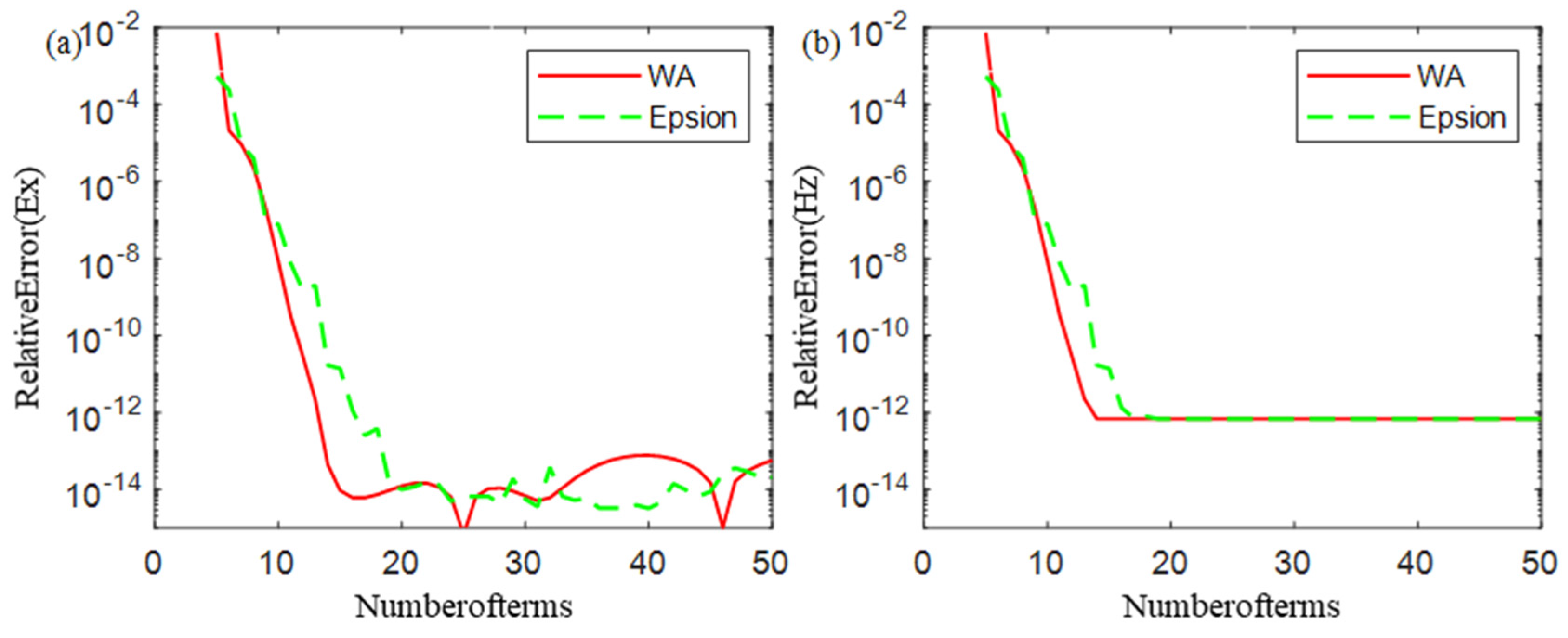
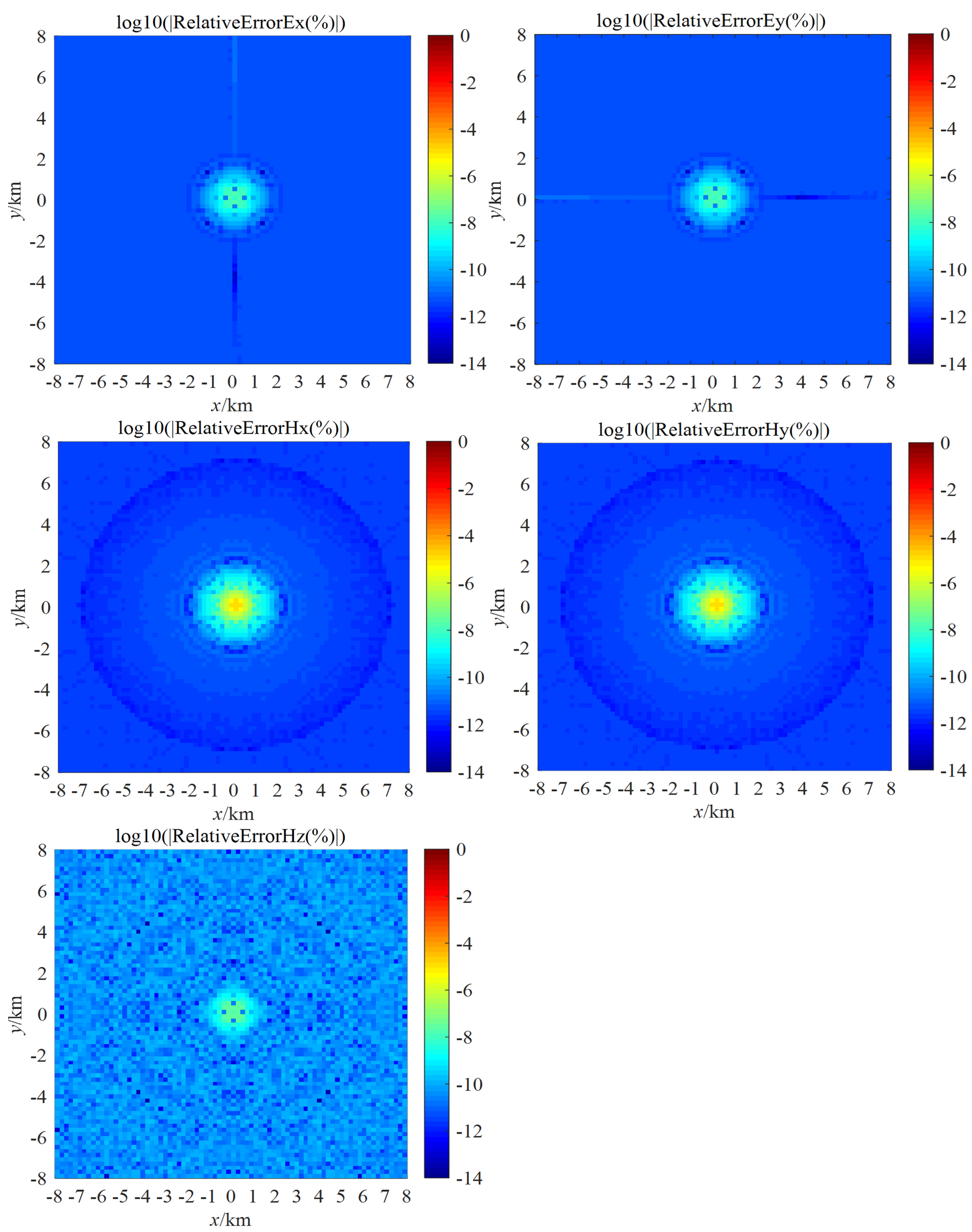
3.1. Accuracy Verification

3.1.1. Horizontal Dipole Source

To verify the correctness of the formulae derivation and the reliability of the code (all of the code mentioned in this article is implemented using MATLAB), the methodology of this paper is compared with the open-source code Dipole1D, an oceanic controlled source electromagnetic method that employs a digital filtering algorithm. To fully determine the numerical stability of the code, the field source is placed at a certain depth, see Figure 2, and the field values of the measurement points at different depths are considered to ensure that the numerical results do not overflow as the depth changes. The field source z = 1750 m with a frequency of 1 Hz was compared to the results for r = 1000 m. The number of Gaussian points is 51, the absolute error $\beta$ is set to ${10}^{-30}$, and the relative error $\alpha$ is set to ${10}^{-10}$.

As can be seen in Figure 3, the results of the six field components are in good agreement with those of Dipole1D at all depths, with no numerical overflow of field values at different depths. The comparative experiment verified the reliability of the derived formula and the WA extrapolation method.

The accuracy of the WA extrapolation algorithm is analyzed below. The accuracy of the WA extrapolation method is mainly affected by the number of Gaussian points and the number of integration intervals. In the following, the accuracy of the electromagnetic field of the electric dipole source is tested in relation to the number of Gaussian points and the number of integration intervals. Sett the model as a uniform half-space, with resistivity of 1000 Ωm, with two sets of transmit–receive distances of 100 m and 1000 m, with an equatorial device, and with frequency of 1 Hz. The number of Gaussian points increases logarithmically from 10 to 1000, and the number of integration intervals increases from 5 to 50. We test the variation law of the relative accuracy of the electric field Ex and magnetic field Hz.

Figure 4 and Figure 5 show the variation in the relative accuracy of the electric dipole source, the horizontal coordinate is the number of integration intervals, the vertical coordinate is the number of Gaussian points, and the color code indicates that the relative error is logarithmic with a base of 10, and the color code in −3 indicates that the relative error is 0.001, and −14 indicates that the relative error is 10–14.

It can be seen that, for both electromagnetic and magnetic fields, as the number of integration intervals and Gaussian points increases, the relative accuracy of the algorithm appears to increase significantly, and the highest relative accuracy achievable is ${10}^{-14}$. After reaching the highest accuracy, increasing the number of integration intervals and Gaussian points will not further improve the field value accuracy. The phenomenon is further illustrated by the obvious horizontal and vertical stripes that appear in the figure. For a transmit–receive distance of r = 100 m, 200 Gaussian integration points are sufficient to achieve the highest accuracy; for a transmit–receive distance of r = 1000 m, 50 Gaussian points are sufficient to achieve the highest accuracy. The larger the transmit–receive distance, the fewer Gaussian integration points are available to achieve the same accuracy, and this phenomenon can be somewhat explained by Equation (22). When r is larger, $J_v(\lambda r)$ decays faster with $\lambda$, which is equivalent to shortening $J_v(\lambda r)$ by a factor of r. Therefore, the whole integral function decays faster with $\lambda$, and the integral is more likely to converge. Therefore, setting the number of Gaussian points to 500 is sufficient to maintain high accuracy in practical calculations.

The following is a comparison of the advantages and disadvantages of the WA algorithm and the epsilon algorithm. Using the same uniform half-space model with a frequency of 1 H, a transmission distance of 100 m, and fixed 500 Gaussian points, the accuracy of the two algorithms was compared under the same number of integration intervals. The results are shown in Figure 6, where “Epsion” represents the existing algorithm. As shown in the figure, the WA extrapolation algorithm has a similar highest accuracy as the epsilon algorithm but can achieve high accuracy in fewer integration intervals.

3.1.2. Vertical Magnetic Dipole Source

Since the magnetic dipole source cannot be calculated in the open source code Dipole1D, this paper compares with the five-component analytical solution generated by a vertical magnetic dipole source at the surface of a uniform half-space. The uniform half-space model, with a resistivity of 1000 $\mathsf{\Omega }·\mathrm{m}$, is computed at a frequency of 1 Hz, comparing the accuracy distribution at different planar locations at the same frequency, with Gaussian points of 51 and a magnetic moment of 1 Am².

The results are shown in Figure 7, where the vertical coordinate is the percentage relative error taken in the logarithm. It can be seen that the numerical accuracy decreases as the transmit–receive distance becomes smaller. For the magnetic dipole source, the numerical integration solution is more accurate, and the relative error level is basically below ${10}^{-12}$ (%) except near the source, which verifies that the principle of duality can be correctly used to calculate the electromagnetic field of the magnetic dipole source. There is a decrease in the accuracy of the electromagnetic fields near the source, which may be because the electromagnetic fields near the source change more rapidly and are more difficult to integrate numerically.

To determine the field value accuracy of the magnetic dipole source in relation to the number of Gaussian points and the number of integration intervals, the effects of the number of integration intervals and the number of Gaussian integration points on the Ex and Hz accuracies were tested for two sets of transmit–receive distance (r = 100 m and r = 1000 m). The results are shown in Figure 8 and Figure 9. The horizontal coordinates are the number of integration intervals, the vertical coordinates are the number of Gaussian points, and the color code indicates that the relative accuracies are taken in the logarithm.

Similar to the horizontal dipole source, the relative accuracy is closely related to the number of Gaussian points and the number of integration intervals, and as the number of Gaussian points and the number of integration intervals increase, the accuracy improves, but there is a maximum accuracy. For a transmit–receive distance of r = 100 m, the highest accuracy in the electric field is about ${10}^{-11}$, and the highest accuracy in the magnetic field is about ${10}^{-10}$. Continuing to increase the number of Gaussian points and integration intervals will not improve the accuracy. As the distance increases, the maximum accuracy increases slightly to ${10}^{-14}$ for both the electric and magnetic fields. A comparison between the epsilon algorithm and the WA algorithm is made and the results are shown in Figure 10, which shows that the WA algorithm has better accuracy for the same number of integration intervals.

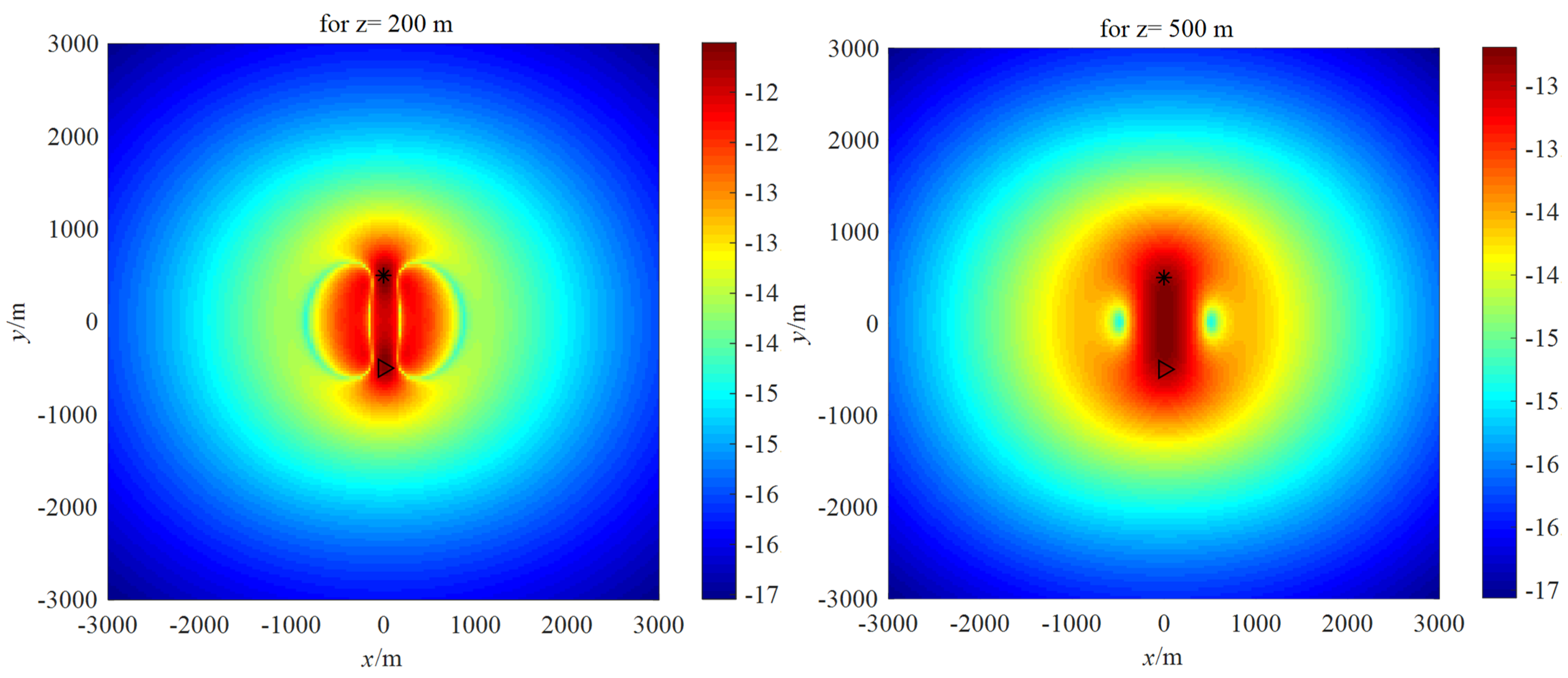
3.2. Algorithmic Applications

3.2.1. Sensitivity Calculation

The sensitivity is the derivative of the data at the receiving point concerning the change in conductivity in a given part of the subsurface [27,28,29,30], and in the continuous case is the Frechet derivative, which represents how the subsurface medium is “illuminated” during the measurement. In the derived integral equation expression, the sensitivity function acts as a weighting function for the conductivity, despite the non-linear correlation between the model and the data. For the sensitivity in the conductivity voxel D, Mcgillivray et al. [31] gave a general formula for calculating the sensitivity by the concomitant method:

$${\displaystyle {\int }_D\left(J_m^{†}·\frac{\partial H}{\partial {\sigma }_k}+J_e^{†}·\frac{\partial E}{\partial {\sigma }_k}\right)dV=}{\displaystyle {\int }_D{E}^{†}·EdV}$$

(45)

where $J_m^{†}$, $J_e^{†}$ denotes the accompanying field source, $E^{†}$ is the accompanying field component, and $E$ denotes the forward field component. Taking the sensitivity of the horizontal electric field Ex of the electric dipole source as an example, the receiving is a horizontal electric field, and the accompanying field source is a horizontal electric dipole source $J_e^{†}=\delta (x_r)\delta (x_r)\delta (z_r)$ placed at the receiving point. By substituting the generated accompanying field $E^{†}$ into Equation (43), the expression for the sensitivity of the electric field component Ex can be obtained:

$${\displaystyle \frac{\partial E_x}{\partial {\sigma }_D}}\left(x,y,z\right)={\displaystyle \frac{{\displaystyle {\int }_D{E}^{†}·EdV}}{i\omega \mu m}}$$

(46)

From this, the sensitivity distribution of any transmitting and receiving device to the conductivity of any voxel D can be obtained. Similarly, the sensitivity of any transmitting and receiving device can be obtained by taking the inner product of the accompanying field and forward field vectors. One-dimensional sensitivity can be obtained by Gaussian integration along the corresponding coordinate axis using a 3D sensitivity function.

In the following, we calculate the sensitivity distribution of a surface electric dipole source transmitting and a surface electric field Ex receiving, with a transmit–receive distance of 1000 m, an equatorial device, a frequency of 10 Hz, and a resistivity of 1000 $\mathsf{\Omega }·\mathrm{m}$, and analyze the distribution pattern of the sensitivity at different depths.

As can be seen in Figure 11, the sensitivity decays rapidly with depth. In the shallow layer, the electric field is mainly sensitive to the region directly below the transmission and receiving points. As the depth increases, the sensitive region gradually shifts from the region directly below the transmit and receive to the middle region of the transmit and receive.

3.2.2. Energy Flow Density Calculation

The electromagnetic field used in the controlled source electromagnetic method is a diffuse field and it is not possible to understand the characteristics of the field with the help of the concepts related to rays in the wavefield, and it is useful to study the energy flow to visualize the behavior of the CSEM field. The propagation of electromagnetic fields is more thoroughly studied in the marine controlled source electromagnetic method, in which the Poynting vectors are a tool for expressing the energy flow to visualize the average energy flow of the electromagnetic field through geological structures.

It has been shown that the time average (over a complete period) of the Poynting vectors is equal to the complex Poynting vector S, which represents the average energy flow in a volume [32]. Chave and Luther used the real part of the complex Poynting vectors to visualize the energy flow in a model of the Earth that contains a low-conductivity lithospheric zone. Weidelt [33] also used energy flow density to demonstrate the fundamental laws of electromagnetic fields in the application of the ocean controlled source electromagnetic method for detecting a hydrocarbon. After calculating the electromagnetic field components, the Poynting vector can be obtained, expressed as:

$$\overline{\mathbf{S}}={\displaystyle \frac{1}{2{\mu }_0}}\mathrm{Re}\left(E\times B^{*}\right)$$

(47)

In the xz-plane at y = 0, the corresponding components can be expressed as:

$${\overline{S}}_x=-{\displaystyle \frac{1}{2{\mu }_0}}\mathrm{Re}\left(E_z{B}_y^{*}\right),\hspace{1em}{\overline{S}}_z=+{\displaystyle \frac{1}{2{\mu }_0}}\mathrm{Re}\left(E_x{B}_y^{*}\right),$$

(48)

Calculate the K-type model with a frequency of 1 Hz, the field source is located at the origin of the coordinates, and the field source is along the x-direction. The parameters are $\left({\rho }_1,{\rho }_2,{\rho }_3\right)=\left(10 \mathsf{\Omega }·\mathrm{m},1000 \mathsf{\Omega }·\mathrm{m},10 \mathsf{\Omega }·\mathrm{m}\right)$, $\left(h_1,h_2\right)=\left(800 \mathrm{m},500 \mathrm{m}\right)$.

The results are shown in Figure 12, where the vector arrows represent only the direction and the color code represents the logarithm of the amplitude of the energy flow density. A clear energy flow channel is formed inside the high resistance layer, similar to the guided wave phenomenon in ocean controlled sources, which means that the electric dipole source has a certain degree of detectability for the high-resistance layer. When the transmit–receive distance is small, the energy flow density basically spreads towards the direction away from the field source similar to the spherical diffusion; when the transmit–receive distance gradually becomes larger, the energy flow density vector gradually turns to the vertical direction, which indicates that the electromagnetic field in the far area basically propagates vertically.

4. Conclusions

The contribution of this article lies in deepening the theoretical basis of electromagnetic field calculation in layered media. By deriving in detail the recursive formula of electromagnetic field in layered media and the conversion formula between Schelkunoff potentials and magnetic vector potential, the significance of interlayer coefficients is clarified, and the application of the duality principle in magnetic dipole source calculation is expanded. These works provide new perspectives and tools for the development of electromagnetic field theory, enriching research methods in fields such as geological exploration and geophysics.

The high-resolution electromagnetic field-calculation algorithm based on the weighted average (WA) extrapolation method proposed in this article not only ensures high accuracy in the calculation of apparent resistivity and sensitivity, and effectively eliminates the influence of numerical errors, but also achieves high-precision calculation of electric dipole sources and magnetic dipole sources in different orientations. Compared with the open-source Dipole1D and traditional epsilon algorithms, this algorithm has faster convergence speed and higher computational efficiency, and can achieve relative accuracy on the order of ${10}^{-10}$ in fewer integration intervals, significantly improving the practicality and reliability of electromagnetic field simulation.

This article further developed calculation methods for sensitivity and Poynting vector, providing powerful tools for in-depth analysis of electromagnetic field response laws. These tools play an irreplaceable role in interpreting electromagnetic exploration data, evaluating detection effectiveness, and optimizing exploration design.

In the later stage, we will further optimize the parameter settings of the WA extrapolation method and explore more efficient algorithm-implementation methods to improve computational efficiency and accuracy. Secondly, we will strengthen the application testing of algorithms in actual geological exploration projects to verify their effectiveness and reliability under complex geological conditions. In addition, we will consider extending the WA extrapolation method to two-dimensional and three-dimensional electromagnetic field calculations to address a wider range of geological structures and exploration needs.

References

1. Kong, F. Hankel transform filters for dipole antenna radiation in a conductive medium. Geophys. Prospect. 2007, 55, 83–89. [Google Scholar] [CrossRef]
2. Løseth, L.; Ursin, B. Electromagnetic fields in planarly layered anisotropic media. Geophys. J. Int. 2007, 170, 44–80. [Google Scholar] [CrossRef]
3. Hunziker, J.; Thorbecke, J.; Slob, E. The electromagnetic response in a layered vertical transverse isotropic medium: A new look at an old problem. Geophysics 2015, 80, F1–F18. [Google Scholar] [CrossRef]
4. Chave, A.D. Numerical integration of related Hankel transforms by quadrature and continued fraction expansion. Geophysics 1983, 48, 1671–1686. [Google Scholar] [CrossRef]
5. Ward, S.H.; Hohmann, G.W. Electromagnetic theory for geophysical applications. In Electromagnetic Methods in Applied Geophysics: Volume 1, Theory; Society of Exploration Geophysicists: Houston, TX, USA, 1988; pp. 130–311. [Google Scholar]
6. Kaufman, A.A.; Keller, G.V. Frequency and Transient Soundings; King, C.-Y., Scarpa, R., Eds.; Elsevier: Amsterdam, The Netherlands, 1983; p. 207. [Google Scholar]
7. Key, K. 1D inversion of multicomponent, multifrequency marine CSEM data: Methodology and synthetic studies for resolving thin resistive layers. Geophysics 2009, 74, F9–F20. [Google Scholar] [CrossRef]
8. Liu, R.; Liu, J.; Wang, J.; Wang, J.; Liu, Z.; Guo, R. 1D electromagnetic response modeling with arbitrary source-receiver geometry based on vector potential and its implementation in MATLAB. Geophysics 2020, 85, F27–F38. [Google Scholar] [CrossRef]
9. Mosig, J. The weighted averages algorithm revisited. IEEE Trans. Antennas Propag. 2012, 60, 2011–2018. [Google Scholar] [CrossRef]
10. Ghosh, D. Inverse filter coefficients for the computation of apparent resistivity standard curves for a horizontally stratified earth. Geophys. Prospect. 1971, 19, 769–775. [Google Scholar] [CrossRef]
11. Key, K. Is the fast Hankel transform faster than quadrature? Geophysics 2012, 77, F21–F30. [Google Scholar] [CrossRef]
12. Weniger, E.J. Nonlinear sequence transformations for the acceleration of convergence and the summation of divergent series. Comput. Phys. Rep. 1989, 10, 189–371. [Google Scholar] [CrossRef]
13. Lucas, S.; Stone, H. Evaluating infinite integrals involving Bessel functions of arbitrary order. J. Comput. Appl. Math. 1995, 64, 217–231. [Google Scholar] [CrossRef]
14. Michalski, K.A. Extrapolation methods for Sommerfeld integral tails. IEEE Trans. Antennas Propag. 1998, 46, 1405–1418. [Google Scholar] [CrossRef]
15. Mosig, J.R.; Michalski, K.A. Sommerfeld integrals and their relation to the development of planar microwave devices. IEEE J. Microw. 2021, 1, 470–480. [Google Scholar] [CrossRef]
16. Golubović, R.; Polimeridis, A.G.; Mosig, J.R. The weighted averages method for semi-infinite range integrals involving products of Bessel functions. IEEE Trans. Antennas Propag. 2012, 61, 5589–5596. [Google Scholar] [CrossRef]
17. Lovat, G.; Celozzi, S. Lucas decomposition and extrapolation methods for the evaluation of infinite integrals involving the product of three Bessel functions of arbitrary order. J. Comput. Appl. Math. 2025, 453, 116141. [Google Scholar] [CrossRef]
18. Kien, P.N.; Lee, S.M. 1DCSEMQWE: 1D Controlled Source Electromagnetic Method in Geophysics Using Quadrature with Extrapolation. SoftwareX 2022, 19, 101128. [Google Scholar] [CrossRef]
19. Michalski, K.; Mosig, J. The Sommerfeld half-space problem revisited: From radio frequencies and Zenneck waves to visible light and Fano modes. J. Electromagn. Waves Appl. 2016, 30, 1–42. [Google Scholar] [CrossRef]
20. Wang, F. Isotropic and Anisotropic Three-dimensional Inversion of Frequency-Domain Controlled-Source Electromagnetic Data Using Finite Element Techniques. Doctoral Dissertation, Fakultät Für Geowissenschaften, Geotechnik und Bergbau der Technischen Universität Bergakademie Freiberg, Saxony, Germany, 2016. [Google Scholar]
21. Abdalla, M. On Hankel transforms of generalized Bessel matrix polynomials. AIMS Math. 2021, 6, 6122–6139. [Google Scholar] [CrossRef]
22. Werthmüller, D.; Key, K.; Slob, E.C. A tool for designing digital filters for the Hankel and Fourier transforms in potential, diffusive, and wavefield modeling. Geophysics 2019, 84, F47–F56. [Google Scholar] [CrossRef]
23. Thukral, R. A family of the functional epsilon algorithms for accelerating convergence. Rocky Mt. J. Math. 2008, 38, 291–307. [Google Scholar] [CrossRef]
24. Brezinski, C.; Redivo-Zaglia, M.; Salam, A. On the kernel of vector ε-algorithm and related topics. Numer. Algorithms 2023, 92, 207–221. [Google Scholar] [CrossRef]
25. Nagid, N.; Belhadj, H. New Approach for Accelerating Nonlinear Schwarz Iterations. Bol. Soc. Parana. Matemática 2020, 38, 51–69. [Google Scholar] [CrossRef]
26. Michalski, K.A.; Mosig, J.R. Efficient computation of Sommerfeld integral tails–methods and algorithms. J. Electromagn. Waves Appl. 2016, 30, 281–317. [Google Scholar] [CrossRef]
27. Hanssens, D.; Delefortrie, S.; Pue, J.D.; Meirvenne, M.C.; Smedt, P.D. Frequency-Domain Electromagnetic Forward and Sensitivity Modeling: Practical Aspects of Modeling a Magnetic Dipole in a Multilayered Half-Space. IEEE Geosci. Remote Sens. Mag. 2019, 7, 74–85. [Google Scholar] [CrossRef]
28. Rincon-Tabares, J.-S.; Velasquez-Gonzalez, J.C.; Ramirez-Tamayo, D.; Montoya, A.; Millwater, H.; Restrepo, D. Sensitivity Analysis for Transient Thermal Problems Using the Complex-Variable Finite Element Method. Appl. Sci. 2022, 12, 2738. [Google Scholar] [CrossRef]
29. Uhm, J.; Oh, J.W.; Min, D.J.; Heo, J. Analysis of sensitivity patterns for characteristics of magnetotelluric (MT) response functions in inversion. Geophys. J. Int. 2023, 233, 1746–1771. [Google Scholar] [CrossRef]
30. Liu, T.T.; Bohlen, T. Time-domain poroelastic full-waveform inversion of shallow seismic data: Methodology and sensitivity analysis. Geophys. J. Int. 2023, 232, 1803–1820. [Google Scholar] [CrossRef]
31. McGillivray, P.; Oldenburg, D.; Ellis, R.; Habashy, T. Calculation of sensitivities for the frequency-domain electromagnetic problem. Geophys. J. Int. 1994, 116, 1–4. [Google Scholar] [CrossRef]
32. Chave, A.D. On the electromagnetic fields produced by marine frequency domain controlled sources. Geophys. J. Int. 2009, 179, 1429–1457. [Google Scholar] [CrossRef]
33. Weidelt, P. Guided waves in marine CSEM. Geophys. J. Int. 2007, 171, 153–176. [Google Scholar] [CrossRef]
Figure 1. Schematic diagram of layered model.
Electronics 13 03827 g001
Figure 2. Schematic diagram of the layered model.
Electronics 13 03827 g002
Figure 3. Horizontal electric dipole (r = 1000 m) electromagnetic field component comparison results. (a) E x component; (b) E y component; (c) E z component; (d) H x component; (e) H y component; (f) H z component.
Electronics 13 03827 g003
Figure 4. Relative error of electric dipole at r = 100 m. (a) Ex accuracy; (b) Hz accuracy.
Electronics 13 03827 g004
Figure 5. Relative error of electric dipole at r = 1000 m. (a) Ex accuracy; (b) Hz accuracy.
Electronics 13 03827 g005
Figure 6. Comparison of acceleration effects of extrapolation methods for electric dipole sources. (a) Ex component accuracy; (b) Hz component accuracy.
Electronics 13 03827 g006
Figure 7. Relative error between the numerical integration solution and the analytical solution for the five components Ex, Ey, Hx, Hy, Hz generated by the VMD.
Electronics 13 03827 g007
Figure 8. Analysis of vertical magnetic dipole accuracy at r = 100 m. (a) Ex accuracy; (b) Hz accuracy.
Electronics 13 03827 g008
Figure 9. Analysis of vertical magnetic dipole accuracy at r = 1000 m. (a) Ex accuracy; (b) Hz accuracy.
Electronics 13 03827 g009
Figure 10. Comparison of acceleration effects of magnetic dipole source extrapolation. (a) Ex accuracy; (b) Hz accuracy.
Electronics 13 03827 g010
Figure 11. Sensitivity distribution at different depths ( represents the position of the transmission source, represents the position of the receiver).
Electronics 13 03827 g011aElectronics 13 03827 g011b
Figure 12. K-model energy flow density.
Electronics 13 03827 g012
Disclaimer/Publisher’s Note: The statements, opinions and data contained in all publications are solely those of the individual author(s) and contributor(s) and not of MDPI and/or the editor(s). MDPI and/or the editor(s) disclaim responsibility for any injury to people or property resulting from any ideas, methods, instructions or products referred to in the content.