A Prediction Model for Pressure and Temperature in Geothermal Drilling Based on Physics-Informed Neural Networks

Abstract

With the global expansion of geothermal energy, accurate prediction of pressure and temperature during drilling has become essential for ensuring the safety and efficiency of geothermal wells. Traditional numerical methods, however, often struggle to handle complex wellbore environments due to their high data demands and limited computational accuracy. To address these challenges, this paper introduces an innovative predictive model based on Physics-Informed Neural Networks (PINNs). By integrating physical laws with deep learning, the model theoretically surpasses the limitations of conventional methods. Trained on pressure and temperature data from a geothermal well in the Xiong’an area, the model demonstrates exceptional accuracy and robustness. Additionally, the model was rigorously tested under extreme wellbore conditions, showcasing its strong generalization capabilities. The findings suggest that PINNs offer a highly advantageous solution for geothermal drilling, with significant potential for practical engineering applications.

1. Introduction

Geothermal energy, with its low carbon emissions and abundant reserves, has been a key renewable energy source globally since the early 20th century. As a clean energy source, geothermal energy not only provides environmental benefits, broad applications, high stability, and recyclability but also holds great potential in combating climate change and reducing greenhouse gas emissions. However, as drilling depth increases, the operational environment within geothermal wells becomes increasingly complex, making the precise measurement of parameters such as temperature and pressure an unprecedented challenge [1,2,3]. The complicated subsurface conditions often lead to measurement errors, which in turn affect wellbore safety and drilling efficiency. Therefore, to further reduce the cost of geothermal drilling and enhance operational safety, it is crucial to establish an accurate and reliable geothermal drilling model. Traditionally, researchers have relied on classical numerical methods such as the finite difference method and the finite element method to solve partial differential equations (PDEs) in wellbore models [4,5]. Zhang and his team (2022) developed a model to simulate the temperature distribution within a geothermal well during simultaneous occurrences of well leakage and wellbore influx. Their model revealed the temperature distribution patterns under these concurrent conditions [6]. Xu et al. (2018) employed the drift flux model to describe gas–liquid two-phase flow and developed a transient, non-isothermal two-phase flow model for dynamically simulating multiphase flow within the wellbore following a gas influx. The model systematically solved the energy conservation equation using the finite difference method [7]. However, these empirical models often suffer from limited generalization capabilities. For example, A’ lvarez del Castillo and colleagues simulated two porosity correlations to calculate pressure gradients and compared the errors between field data and simulated results, finding average accuracy errors as high as 12.8% and 14.6% [8]. With the rapid advancement of artificial intelligence, more researchers are turning to deep learning techniques for geothermal drilling modeling, aiming to improve model accuracy and adaptability through data-driven approaches to tackle the complexities of geological conditions and drilling operations.

Deep learning, specifically artificial neural networks, is widely applied in various fields, including computer vision, natural language processing (NLP), speech recognition, autonomous driving, robotics, and oil and gas exploration and development. ANNs offer several advantages in wellbore modeling, including the ability to handle complex nonlinear problems, perform efficient computations, and reduce reliance on physical parameters through data-driven modeling.

Pavel Spesivtsev and his team (2018) developed an artificial neural network with two hidden layers, trained using data generated with a transient wellbore flow numerical simulator. After training, the neural network was employed to predict bottomhole pressure, one of the key parameters in wellbore flow [9]. Hakki Aydin et al. (2020) developed a proxy artificial neural network model based on wellhead data to monitor reservoir temperature and pressure. The model’s application and benefits were demonstrated using a geothermal production well located in the Alaşehir geothermal field in Turkey [10]. Bassam A. et al. (2015) proposed a method for predicting pressure drops in flowing geothermal wells based on artificial neural networks (ANNs) and wellbore numerical simulations. They set up two neural networks, ANN1 and ANN2, with five and six input variables, respectively. Using the same production data, predictions were made with both neural networks and the numerical simulator (GEOWELLS). The results concluded that the ANN2 model performed better [11]. Li et al. (2022) employed a genetic algorithm to optimize a multi-layer feedforward neural network, developing a GA-BP neural network model for drilling kick prediction based on multi-parameter integration [12]. Mahmoud et al. (2024) introduced an innovative model for predicting pore pressure using artificial neural networks, achieving high accuracy in pore pressure forecasting [13]. Muojeke et al. (2020) developed a data-driven kick detection model by integrating artificial neural networks (ANNs), binary classifiers, and real-time monitoring of drilling flow parameters, a crucial step towards enhancing drilling safety [14]. Meanwhile, Zhu et al. (2023) proposed a workflow that integrates wellbore flow mechanisms as physical constraints, offering a more stable and hydraulically consistent bottomhole pressure prediction. They also employed particle swarm optimization to globally solve the neural network’s weights and biases, eliminating the need to compute the loss function’s derivatives [15].

In recent years, with the widespread application of artificial neural networks across various fields, numerous new neural network architectures have emerged, such as Convolutional Neural Networks (CNNs), Recurrent Neural Networks (RNNs), and their variants (like Long Short-Term Memory networks (LSTMs) and Gated Recurrent Units (GRUs)), Deep Neural Networks (DNNs), Functional Link Neural Networks (FLNNs), and Adaptive Neuro-Fuzzy Inference Systems (ANFISs), among others [16,17,18].

In 2019, Raissi M. et al. introduced Physics-Informed Neural Networks (PINNs), which are trained to solve supervised learning tasks while adhering to the physical laws described via nonlinear PDEs [19]. Karniadakis G.E. (2021) pointed out that neural networks requiring large amounts of data for training are not always suitable for scientific problems. Although purely data-driven models are well suited for fitting observed results, they may exhibit poor generalization performance due to extrapolation or observational biases, leading to predictions that are physically inconsistent or unreliable. Physics-Informed Neural Networks (PINNs) can be trained using additional information derived from enforcing physical laws (e.g., at random points in continuous space–time domains). This physics-based learning integrates noisy data with mathematical models and implements them through neural networks [20]. Cai S.Z. et al. (2021) reviewed the application of Physics-Informed Neural Networks (PINNs) in fluid mechanics and implemented these methods using PINNs. They concluded that in the near future, PINNs could be used to address large-scale industrial complexity problems that traditional CFD methods cannot solve [21]. As shown in Figure 1, PINNs, as a type of deep learning network, differ from traditional computational methods in that they do not require extensive theoretical foundations; they often exhibit good robustness even when driven by imperfect data, thus effectively combining the strengths of physical laws and artificial neural networks. Zhang et al. (2023) proposed a nested structure for PINNs with a loss model, integrating an adaptive weighting method for transient analysis of pipeline networks [22]. Cai et al. (2021) introduced the application of Physics-Informed Neural Networks (PINNs) in heat transfer problems. Nazari et al. (2024) investigated a new hybrid model based on PINNs to simulate multiphase mass flow in offshore oil and gas fields, aiming to characterize the mass flow dynamics in production wellbores [23,24].

Based on the studies mentioned earlier, although artificial neural networks have demonstrated good application performance in wellbore modeling, their primary drawback lies in the typically large datasets required for training, which can be impractical in complex environments such as geothermal drilling. Additionally, traditional physical computation methods are computationally intensive and often lack precision. To address these issues, this paper establishes a model based on Physics-Informed Neural Networks (PINNs). The model utilizes the backpropagation algorithm to compute gradients and the Adam optimizer for adaptive weight updates, while incorporating L2 regularization to limit the size of weights and biases, thereby preventing overfitting. The PINN model combines the advantages of machine learning in handling complex data with the modeling capabilities based on physical principles, enabling accurate predictions of pressure and temperature within geothermal wellbores. This paper also compares the prediction results of the model with those from traditional finite difference methods and existing ANN models and tests the model’s generalization through a real-world case study.

The innovations of this paper are as follows:

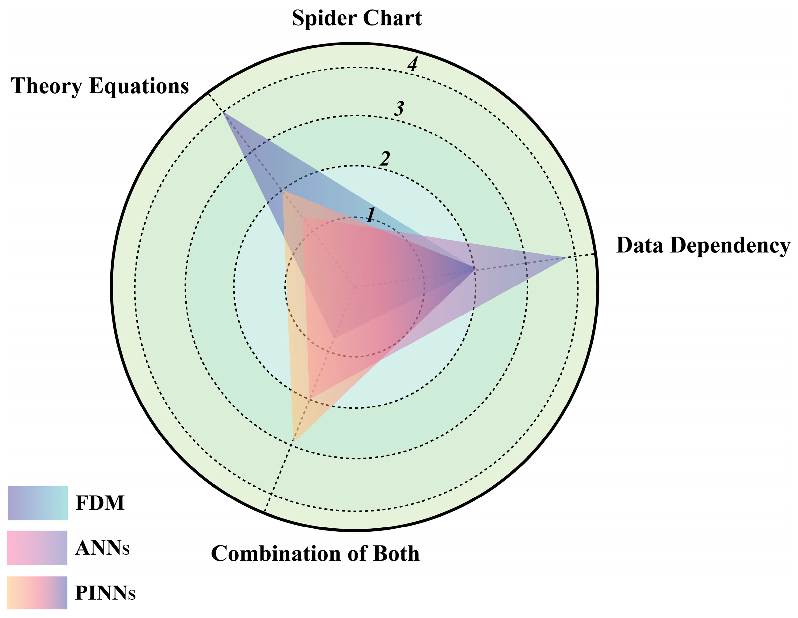
• It is the first to apply Physics-Informed Neural Networks (PINNs) to geothermal drilling modeling;
• The model enhances applicability in situations with limited data by reducing dependence on large-scale datasets;
• The predictive capabilities of ANNs and PINNs were tested through a real-world case, validating the model’s generalization ability.

2. Methodology

A clear understanding of the flow dynamics within geothermal wellbores is essential for developing a wellbore prediction model. Accordingly, Section 2.1 outlines the key concepts of gas–liquid two-phase flow in geothermal systems. Section 2.2 provides an in-depth description of the theoretical foundations and architecture of Physics-Informed Neural Networks (PINNs).

2.1. Gas–Liquid Two-Phase Flow

Gas–liquid two-phase flow refers to the simultaneous flow of gas and liquid within the same pipe or channel, a phenomenon that significantly impacts the pressure and temperature distribution in geothermal drilling. To better simulate and predict this complex flow behavior, this study employs the conservation equations of mass, momentum, and energy to describe the fluid dynamics. These equations, commonly used in fluid mechanics (as summarized systematically by Tonkin et al. in 2021, defining two-phase flow parameters in wellbores, and in 2023, when they developed a transient wellbore simulator) [25,26]. These serve as the theoretical foundation for constructing the Physics-Informed Neural Network (PINN) model.

The mass conservation equation ensures that the total mass of both gas and liquid remains constant over time and space.

Mass conservation equation:

$${\displaystyle \frac{\partial }{\partial t}}\left({\rho }_g{\alpha }_g+{\rho }_l{\alpha }_l\right)+{\displaystyle \frac{\partial }{\partial x}}\left({\rho }_g{{\alpha }_{g}v}_g+{\rho }_l{{\alpha }_{l}v}_l\right)=0$$

(1)

ρ_g and ρ_l are the densities of the gas phase and liquid phase, respectively. v_g and v_l are the velocities of the gas phase and liquid phase, respectively. α_g and α_l are the cross-sectional gas content and cross-sectional liquid content.

The momentum conservation equation explains how forces acting on the fluid, such as pressure and friction, affect its movement.

Momentum conservation equation:

$${\displaystyle \frac{\partial }{\partial t}}\left({\rho }_g{{\alpha }_{g}v}_g+{\rho }_l{{\alpha }_{l}v}_l\right)+{\displaystyle \frac{\partial }{\partial x}}\left(P+{\rho }_g{\alpha }_g{v}_g^2+{\rho }_l{{\alpha }_{l}v}_l^2\right)=-{\rho }_m{v}_{m}g\sin \theta -{\displaystyle \frac{f{\rho }_m{v}_m\left|v_m\right|}{2D}}$$

(2)

P is the wellbore pressure; ρ_m and v_m are the density and velocity of the gas–liquid mixture, respectively; f is the wellbore friction coefficient. The specific form of f can be obtained from Reference [5]; and D is the wellbore diameter.

The energy conservation equation accounts for the exchange of energy between the fluid and its surrounding environment, including heat transfer and kinetic energy.

Energy conservation equation:

$${\displaystyle \frac{\partial }{\partial t}}\left[{\rho }_g{\alpha }_g\left(e_g+{\displaystyle \frac{1}{2}}{v}_g^2\right)+{\rho }_l{\alpha }_l\left(e_l+{\displaystyle \frac{1}{2}}{v}_l^2\right)\right]+{\displaystyle \frac{\partial }{\partial x}}\left({\rho }_g{{\alpha }_{g}v}_g{h}_{Tg}+{\rho }_l{{\alpha }_{l}v}_l{h}_{Tl}\right)+{\displaystyle \frac{Q}{\pi r_i^2}}=0$$

(3)

e_g and e_l are the specific internal energies of the gas and liquid phases, respectively. h_Tg and h_Tl are the total specific enthalpies, defined as the sum of the specific enthalpy, kinetic energy, and potential energy. Q represents the energy transferred from the formation to the interior of the wellbore, and its specific form is based on the description by Hasan et al. [27]; r_i is the wellbore radius.

2.2. Physics-Informed Neural Networks

Define a function u(x, t), which represents a physical quantity (such as temperature, pressure, etc.) at a spatial position x and time t. This paper assumes that this function is described by the following differential equation:

$$P\left(u\left(x,t\right),\lambda \right)=0$$

(4)

where P (⋅) is a differential operator that describes the physical system, and λ represents physical parameters, which may be unknown or difficult to measure directly.

By constructing a neural network $𝒩$$𝒩$(x, t; θ), where θ = {w,b} is the set of network parameters, including the weights w and biases b of all layers, this network is used to approximate the unknown function u(x, t), yielding an approximate solution u_θ(x, t). The difference between the network output u_θ(x, t) and the true value u(x, t) is measured with the loss function. Additionally, the network output must satisfy the physical equation P (u_θ(x, t), λ) = 0. Due to approximation errors, this equation may not hold exactly, which introduces a second component of the loss function, the physical loss. When the model has initial conditions u(x, 0) = g(x) and boundary conditions u(x, t) = h(x, t), the PINNs incorporate the residuals of these conditions into the loss function to ensure that the neural network’s output satisfies both initial and boundary conditions. The final loss formula is as follows:

$$\mathcal{L}\left(\theta \right)={MSE}_u+{MSE}_P+{MSE}_{ic}+{MSE}_{bc}$$

(5)

In Equation (5), the four terms on the right side of the equals sign are as follows: MSE_u represents the data loss, MSE_P represents the physical equation loss, MSE_ic represents the initial condition loss, and MSE_bc represents the boundary condition loss. Their respective expressions are shown as follows:

$${MSE}_u={\displaystyle \frac{1}{N}}\sum _{i=1}^N{\left(u_{\theta }\left(x_i,t_i\right)-u_i\right)}^2$$

(6)

$${MSE}_P={\displaystyle \frac{1}{M}}\sum _{j=1}^M{\left(P\left(u_{\theta }\left(x_j,t_j\right),\lambda \right)\right)}^2$$

(7)

$${MSE}_{ic}={\displaystyle \frac{1}{K}}\sum _{k=1}^K{\left(u_{\theta }\left(x_k,t_0\right)-u_0\left(x_k\right)\right)}^2$$

(8)

$${MSE}_{bc}={\displaystyle \frac{1}{S}}\sum _{s=1}^S{\left(u_{\theta }\left(x_b,t_s\right)-u_b\left(t_s\right)\right)}^2$$

(9)

In the equations, N represents the observed data, providing the true values that the neural network aims to fit, primarily for the data-driven component. M, K, and S denote the sampling points selected to ensure the neural network’s output adheres to the physical constraints and satisfies the governing physical equations. u_i refers to the measured values at the data points, while u₀ and u_b represent the initial and boundary conditions of the wellbore model, respectively. The schematic diagram of the structure of the Physics-Informed Neural Networks (PINNs) is shown in Figure 2. During the training process, the network receives input data points (x, t) and outputs the corresponding physical quantity u_θ(x, t). The network’s parameters θ are then adjusted by comparing the output with the true observed data (if available) and by checking whether the output satisfies the constraints of the physical equations. After several training iterations, the network converges to a solution that both fits the data and adheres to the physical laws.

3. Wellbore Prediction Model Based on PINNs

This section primarily includes an evaluation of the effectiveness of Physics-Informed Neural Networks (PINNs) in predicting pressure and temperature within the wellbore.

Firstly, Section 3.1 discusses the design of neural network parameters and structures specific to wellbore modelling. In Section 3.2, the training data setup for the predictive model is introduced, followed by a description of its loss function design. Finally, Section 3.3 analyses the prediction results of the wellbore model.

3.1. PINN Design

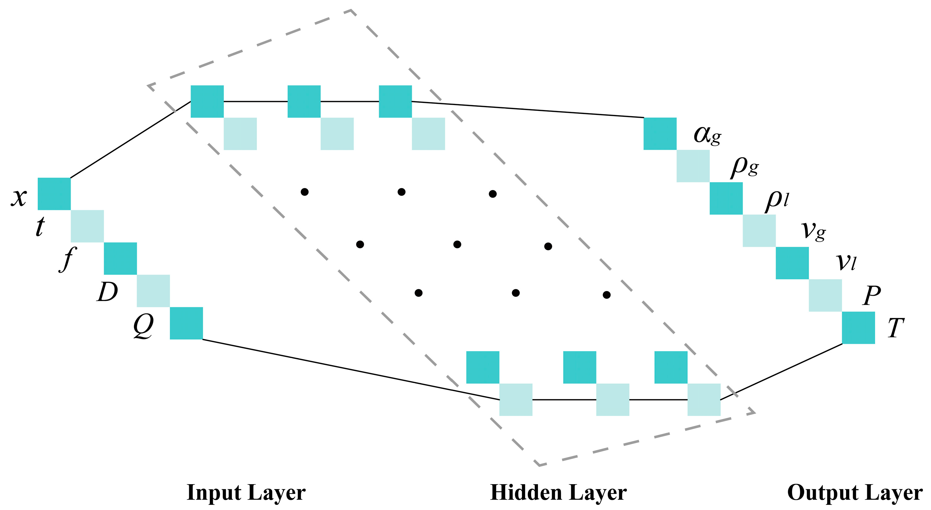
3.1.1. Network Input and Output Parameters

The first step is to determine the input and output parameters of the network. Based on the physical equations to be fitted, the output parameters of the neural network are determined as seven physical quantities: {α_g, ρ_g, ρ_l, v_g, v_l, P, T} (gas volume fraction, gas density, liquid density, gas velocity, liquid velocity, pressure, and temperature). Since fitting the physical equations also requires the values of Q, f, and D, input parameters for the network are {x, t, f, D, Q}. It is assumed that the wellbore wall roughness in this study is 0.00175 mm.

3.1.2. Network Structure

With the input and output parameters now determined, the next step is to establish the network structure. Given that the physical equations to be fitted are highly nonlinear partial differential equations, the network is configured with three hidden layers, each containing 20 neurons. This configuration was identified as optimal after several adjustments. Increasing the number of network layers enhances the model’s ability to tackle complex nonlinear problems. For Physics-Informed Neural Networks (PINNs), deeper networks are more effective at capturing the intricate temperature and pressure variations in geothermal drilling, while still maintaining adherence to the physical constraints. However, excessive layers may lead to overfitting or heightened computational costs. Thus, a network with three hidden layers was chosen in the experiment to strike a balance between model complexity and computational efficiency. Each layer uses the Rectified Linear Unit (ReLU) activation function, which introduces nonlinearity, enabling the network to learn and represent complex patterns. While functions like tanh and sin often perform well when handling physics-informed constraints, ReLU is more suited to general deep learning tasks. Its simplicity and efficiency help mitigate the vanishing gradient problem in deep networks. Additionally, L2 regularization was applied in each hidden layer, incorporating the sum of squared weights as a penalty term in the loss function to limit model complexity and prevent overfitting to the training data. As a result, the final network structure is shown in Figure 3.

3.2. Network Training

3.2.1. Training Data Setup

In this study, the well that was used for the experiments is from a geothermal well in the Xiong’an area. The specific well parameters are shown in

Table 1. Parameters of a geothermal well in the Xiong’an area.

Parameter	Value
Depth (m)	3500
Wellbore diameter (mm)	222
Drillpipe ID (mm)	119
Drillpipe OD (mm)	159
Gas injection rate (m3/s)	0.263
Surface temperature (°C)	25
Bottomhole temperature (°C)	71.1
Casing ID (mm)	306
Casing OD (mm)	350
Mud density (kg/m3)	1066.45

. The experimental assumptions are as follows: the flow inside the wellbore is turbulent; the slip between gas and liquid phases is neglected; and the wellbore diameter remains unchanged.

The training data selected for the experiment are obtained by solving the geothermal wellbore gas–liquid two-phase flow model using the finite difference method combined with the Newton–Raphson iteration method on a discrete grid [3]. To assess the robustness of the model to perturbations, Gaussian noise with a standard deviation of 5% of the data value was added to the training dataset to simulate measurement errors and uncertainties in real-world conditions. After adding the noise, the data were normalized using a linear scaling method between 0 and 1. This normalization not only stabilized the model’s training process on noisy data but also effectively reduced the risks of gradient vanishing and gradient explosion, thereby improving the model’s adaptability to the complex geothermal well environment.

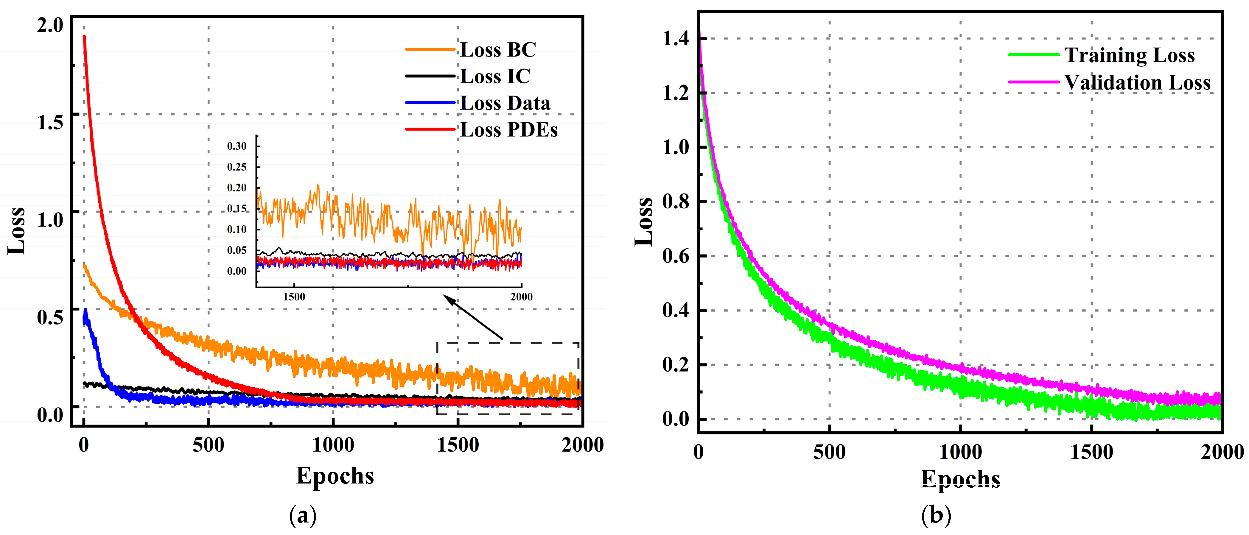
3.2.2. Model Loss Function

Incorporating the mass, momentum, and energy conservation equations for the gas–liquid two-phase flow mentioned in Section 2.1, along with the output parameters shown in Figure 3, the loss function expression for transient flow can be formulated as follows:

$$\mathcal{L}\left(\theta \right)={\mathcal{L}}_d\left(\theta \right)+{\delta }_1{\mathcal{L}}_P\left(\theta \right)+{{\delta }_2\mathcal{L}}_I\left(\theta \right)+{{\delta }_3\mathcal{L}}_{bc}\left(\theta \right)$$

(10)

In Equation (10), each term represents the sum of the respective losses, with δ₁, δ₂, and δ₃ representing the weighting coefficients for the physical equation loss, initial condition loss, and boundary condition loss, respectively. These weights can be customized or adjusted during training, as referenced from the work of Wang et al. [28,29]. In Physics-Informed Neural Networks (PINNs), the data loss term is typically not weighted, to ensure that the model consistently bases its learning on the training data. However, the weights for the physical loss terms need to be dynamically adjusted during training to strike a balance between physical constraints and data fitting. This approach helps the model accurately predict and maintain a good fit with actual observation data, even under complex physical conditions, such as those within a geothermal wellbore.

$ℒ$_P(θ) represents the sum of the losses for the wellbore gas–liquid two-phase flow conservation equations. The losses for the three conservation equations are represented by $ℒ$_P1(θ), $ℒ$_P2(θ), and $ℒ$_P3(θ), respectively. The specific forms are shown in the following equations.

$${\mathcal{L}}_{P1}\left(\theta \right)={\displaystyle \frac{1}{M}}\sum _{i=1}^M{\left({\displaystyle \frac{{\mathcal{N}\mathcal{N}}_{\left({\rho }_g{\alpha }_g+{\rho }_l{\alpha }_l\right)}\left(x_i,t_i;\theta \right)}{\partial t_i}}+{\displaystyle \frac{{\mathcal{N}\mathcal{N}}_{\left({\rho }_g{{\alpha }_{g}v}_g+{\rho }_l{{\alpha }_{l}v}_l\right)}\left(x_i,t_i;\theta \right)}{\partial x_i}}\right)}^2$$

(11)

$${\mathcal{L}}_{P2}\left(\theta \right)={\displaystyle \frac{1}{M}}\sum _{i=1}^M{\left({\displaystyle \frac{{\mathcal{N}\mathcal{N}}_{{\rho }_g{{\alpha }_{g}v}_g+{\rho }_l{{\alpha }_{l}v}_l}\left(x_i,t_i;\theta \right)}{\partial t_i}}+{\displaystyle \frac{{\mathcal{N}\mathcal{N}}_{P+{\rho }_g{\alpha }_g{v}_g^2+{\rho }_l{{\alpha }_{l}v}_l^2}\left(x_i,t_i;\theta \right)}{\partial x_i}}-{\rho }_m{v}_{m}g\mathit{sin}\theta -{\displaystyle \frac{f{\rho }_m{v}_m\left|v_m\right|}{2D}}\right)}^2$$

(12)

$${\mathcal{L}}_{P3}\left(\theta \right)={\displaystyle \frac{1}{M}}\sum _{i=1}^M{\left({\displaystyle \frac{{\mathcal{N}\mathcal{N}}_{{\rho }_g{\alpha }_g\left(e_g+\frac{1}{2}{v}_g^2\right)+{\rho }_l{\alpha }_l\left(e_l+\frac{1}{2}{v}_l^2\right)}\left(x_i,t_i;\theta \right)}{\partial t_i}}+{\displaystyle \frac{{\mathcal{N}\mathcal{N}}_{{\rho }_g{{\alpha }_{g}v}_g{h}_{Tg}+{\rho }_l{{\alpha }_{l}v}_l{h}_{Tl}}\left(x_i,t_i;\theta \right)}{\partial x_i}}+{\displaystyle \frac{Q}{\pi r_i^2}}\right)}^2$$

(13)

In the three equations, $𝒩$$𝒩$_(⋅)(x_i, t_i; θ) represents the mathematical operations performed on the results predicted via the neural network.

The PINN model developed in this study was implemented using MATLAB 2023 software. During the training phase, the ADAM optimizer was employed for initial model training. The ADAM optimizer adapts the learning rate, allowing it to converge quickly to an optimal parameter space. The data were divided into multiple batches for training, with each batch performing a weight update. This batch training method allowed the ADAM optimizer to execute multiple weight updates within each epoch. Throughout the training process, 2000 epochs were conducted, with each epoch including 150 batch updates, resulting in a total of 300,000 ADAM optimizer updates. L2 regularization was introduced to limit excessive growth of model parameters by adding a penalty term on weights, thereby enhancing the model’s generalization capability. Additionally, an adaptive loss function weight adjustment method based on gradient magnitude was employed to ensure that the model could learn various tasks or physical constraints in a balanced manner during different training stages. This approach prevented overfitting to a specific loss term and helped the model achieve a balance between physical consistency and prediction accuracy. The specific prediction workflow of the PINN wellbore model is illustrated in Figure 4.

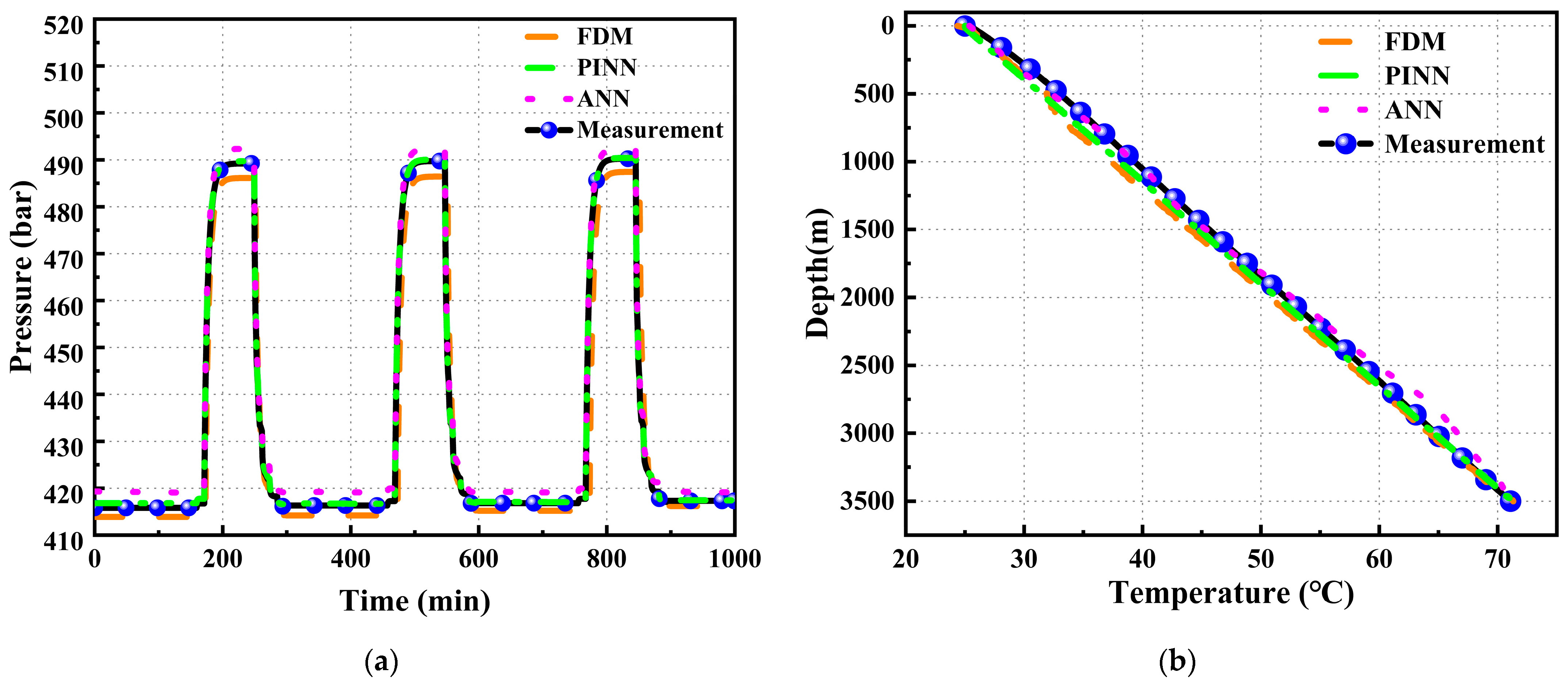
3.3. Prediction Model Validation Analysis

Figure 5a depicts the variation curves of the total training loss and validation loss with the number of iterations for 3000 sample points. Since the total loss comprises data loss, physical equation loss, initial condition loss, and boundary condition loss, Figure 5b illustrates the respective loss values for each component as they change with iterations. Under the optimal network structure, it can be observed from Figure 5a that at the early stages of training, the total loss is influenced by the varying weighting coefficients of the different loss components. Initially, the combined effects of boundary condition loss, initial condition loss, data loss, and physical equation loss cause the total loss to decrease rapidly. By iteration 1000, the data loss, boundary condition loss, and initial condition loss begin to level off and approach convergence, with physical equation loss becoming the primary factor influencing the network model. This aligns with our initial expectations that the network output should satisfy not only the data and other conditions but also adhere to physical laws. As the physical model stabilizes after 1500 iterations, the total training loss and validation loss, as shown in Figure 5b, also gradually level off, ultimately reaching the desired result. Based on the calculations, the total training loss MSE_t is 3.37 × 10⁻³, and the validation loss MSE_v is 6.46 × 10⁻³. In Figure 5b, the validation loss is slightly larger than the training loss, indicating that the model has good generalization ability on the validation set.

The temperature and pressure data predicted by the network are denormalized to obtain the final prediction results. These results are then compared with the temperature and pressure calculation results obtained using the finite difference method combined with the Newton–Raphson method from Reference [3], the ANN model prediction results established by Aydin et al. (2019) [10], and the actual temperature and pressure data. The comparison of the predicted results is shown in the comparison chart in Figure 6.

As illustrated in Figure 6a, both neural network-based methods show strong performance in fitting the measured curve of bottomhole pressure over time. Initially, during the first 200 min, the prediction errors from the neural networks are greater than those from the traditional finite difference method. However, as time progresses and the networks undergo more training, the prediction errors steadily decrease, eventually surpassing the accuracy of the finite difference method. The mean relative error (MRE) for the finite difference method, combined with the Newton–Raphson technique, is 1.491%. When data are scarce, the advantage of Physics-Informed Neural Networks (PINNs) becomes particularly apparent. As shown in the figure, from the early stages of training to the final stages, the PINN consistently achieves lower prediction errors compared to the artificial neural network (ANN). This is because the PINN not only relies on data but also incorporates physical constraints, such as the laws of mass and energy conservation, into its loss function. This approach ensures that the model retains physical consistency even when handling the complex conditions present in geothermal wells. The incorporation of these physical laws allows the PINN to compensate for limited data, providing more accurate predictions. In contrast, the ANN’s reliance solely on data means it struggles when faced with data scarcity, leading to poorer performance. Based on our results, the MRE for the PINN is 0.24%, while the MRE for the ANN stands at 0.481%.

Figure 6b presents the temperature profile along the depth of the wellbore, obtained using three different methods. As with the pressure predictions in Figure 6a, the early stages of training show larger temperature prediction errors for the neural networks compared to the finite difference method. However, a closer comparison of the two machine learning methods reveals that the PINN offers greater overall stability, with its error steadily decreasing as training continues. The PINN’s superior performance in complex geological conditions can be attributed to its ability to manage nonlinear challenges, while the integration of physical constraints ensures that its predictions remain consistent with global physical laws. Moreover, the sources of error differ between the ANN and PINN. In the ANN, errors arise primarily due to the model’s inability to fully grasp underlying patterns when faced with sparse or low-quality data. Conversely, the PINN’s errors are mainly encountered in the early stages of training, as the network has yet to fully learn how to balance both physical constraints and data. Nevertheless, as training progresses, the PINN rapidly reduces its errors, ultimately delivering more stable and accurate predictions. The MREs for the three methods are 1.323%, 0.824%, and 1.097%, respectively.

4. Results and Discussion

4.1. Network Test

To rigorously assess the generalization capability of the PINN model developed in this study, the slimhole geothermal well SNLG87-29, as documented by Garg et al. [30], was selected. The critical parameters of this well are detailed in

Table 2. Parameters of SNLG87-29 well.

Parameter	Value
Depth (m)	248.4
Vertical depth (m)	248.4
Angle with vertical (degrees)	0
0–159.7 m Internal diameter (mm)	102
159.7–248.4 m Internal diameter (mm)	99
Depth (m)	248.4
Surface temperature (°C)	22
Bottomhole temperature (°C)	163.5

.

As shown in Table 2, the temperature increases steadily with depth. In a shut-in condition, the surface temperature stabilizes at 22 °C, but as the drilling depth reaches approximately 250 m, the temperature rises significantly to 163.5 °C. During circulation drilling, the wellhead temperature reaches as high as 135 °C. The purpose of selecting this well is to test the performance of the network model under extreme conditions. The test results are presented in Figure 7.

As shown in Figure 7a, during the initial stages of model training, the finite difference method outperforms the other methods in terms of prediction accuracy. This is because the finite difference method relies directly on explicit mathematical equations and physical laws, enabling it to converge quickly and provide high-precision predictions in the early stages. However, as training progresses, the prediction accuracy of the Physics-Informed Neural Network (PINN) gradually surpasses that of the finite difference method and traditional artificial neural networks. The PINN effectively extracts information from the data while leveraging physical laws to refine its predictions, thus progressively improving its accuracy. The MREs for the three different methods are as follows: 1.824%, 0.427%, and 0.862%.

Figure 7b illustrates the relationship between temperature and depth as predicted via the three methods. The Physics-Informed Neural Network (PINN) demonstrates outstanding performance across the entire depth range, particularly as depth increases, where its predictions closely match the actual measured data. This highlights its superiority in handling complex nonlinear problems when integrated with physical information. In contrast, the artificial neural network (ANN), although initially rough in its predictions at shallow depths, gradually improves as depth increases, but its overall accuracy still lags behind that of the PINN. This indicates that, given the same data, the PINN significantly outperforms the ANN, especially in predicting temperatures under complex geological conditions, making the PINN the optimal choice. The calculated MREs for the three different prediction methods are as follows: 0.521%, 0.359%, and 0.777%.

4.2. Discussion

The Physics-Informed Neural Network (PINN) model developed in this study has demonstrated outstanding predictive performance in the context of geothermal drilling, owing to its ability to integrate physical laws with deep learning techniques. When compared with traditional methods such as the finite difference method (FDM) and artificial neural networks (ANNs), the PINN model stands out for its higher accuracy and robustness, particularly in situations where data are sparse. With mean relative errors (MRE) of 0.24% for pressure prediction and 0.82% for temperature, the model proves adept at handling the complexities of the wellbore environment, compensating for data limitations by embedding physical constraints, thereby enhancing predictive accuracy.

In contrast to other approaches found in the literature, the strength of the PINN model lies in its ability to combine physical equations with a data-driven framework—something that many conventional techniques do not achieve. For instance, the model proposed by Zhang et al. [6]. relies on wellbore leakage and influx conditions to simulate temperature distribution, providing useful insights but with limited general applicability. Similarly, Xu et al.’s [7] transient non-isothermal two-phase flow model struggles to adapt under more complex geological conditions. In contrast, the PINN model presented here integrates physical knowledge with neural network methodologies, offering improved generalization and maintaining strong performance in challenging scenarios.

A key strength of the PINN model is its capacity to address both nonlinear challenges and the scarcity of data, making it especially suitable for intricate engineering problems such as geothermal drilling. However, it does have its limitations. In the early stages of training, the model tends to exhibit larger errors, likely due to the time required to reconcile the physical constraints with data fitting. Additionally, the model is highly sensitive to hyperparameters, which suggests future work could focus on refining the model architecture and training strategies to enhance stability and computational efficiency.

5. Conclusions

This study innovatively combines physical knowledge with deep learning, successfully overcoming the reliance of traditional numerical methods on large datasets, thereby improving predictive accuracy and efficiency in complex geological conditions. During the model training process, actual data from geothermal wells in the Xiong’an area were utilized, further enhancing the model’s adaptability and stability. The mean relative error (MRE) for pressure prediction in the Xiong’an wells is 0.24%, while for temperature prediction it is 0.82%.

The PINN model not only theoretically combines the advantages of physical laws and deep learning but also demonstrates exceptional generalization capability and prediction accuracy in practical applications. Rigorous testing with extreme wellbore data from the SNLG87-29 well reveals that the PINN-based geothermal well prediction model achieved mean relative errors of 0.20% for pressure and 0.75% for temperature, showcasing outstanding predictive performance. This achievement validates the superiority of PINNs in addressing complex nonlinear geological problems, providing a precise solution for engineering applications in geothermal drilling.

Future research will focus on further optimizing the model structure and training strategies to explore the broader application potential of PINNs under even more complex conditions, thus advancing their development in the geothermal sector.

References

1. Xu, C.; Li, J.; Yang, R.-Z.; Chen, J.-R.; Tan, H. An Improved Fracture Seismic Method for identifying the drilling targets of medium-deep geothermal resources: A case study on heishan geothermal area. Geothermics 2024, 120, 103019. [Google Scholar] [CrossRef]
2. Zuo, Y.-H.; Sun, Y.-G.; Zhang, L.-Q.; Zhang, C.; Wang, Y.-C.; Jiang, G.-Z.; Wang, X.-G.; Zhang, T.; Cui, L.-Q. Geothermal resource evaluation in the Sichuan Basin and suggestions for the development and utilization of abandoned oil and gas wells. Renew. Energy 2024, 225, 120362. [Google Scholar] [CrossRef]
3. Yuan, Y.; Li, W.-Q.; Zhang, J.-W.; Lei, J.-K.; Xu, X.-H.; Bian, L.-H. A Novel Geothermal Wellbore Model Based on the Drift-Flux Approach. Energies 2024, 17, 3569. [Google Scholar] [CrossRef]
4. Chen, X.; Wang, S.-W.; He, M.; Xu, M.-B. A comprehensive prediction model of drilling wellbore temperature variation mechanism under deepwater high temperature and high pressure. Ocean. Eng. 2024, 296, 117063. [Google Scholar] [CrossRef]
5. Akbar, S.; Fathianpour, N.; Al-Khoury, R. A finite element model for high enthalpy two-phase flow in geothermal wellbores. Renew. Energy 2016, 94, 223–236. [Google Scholar] [CrossRef]
6. Zhang, Z.; Wang, X.; Xiong, Y.-M.; Peng, G.; Wang, G.-R.; Lu, J.-S.; Zhong, L.; Wang, J.P.; Yan, Z.-Y.; Wei, R.-H. Study on borehole temperature distribution when the well-kick and the well-leakage occurs simultaneously during geothermal well drilling. Geothermics 2022, 104, 102441. [Google Scholar] [CrossRef]
7. Xu, Z.-M.; Song, X.-Z.; Li, G.-S.; Wu, K.; Pang, Z.-Y.; Zhu, Z.-P. Development of a transient non-isothermal two-phase flow model for gas kick simulation in HTHP deep well drilling. Appl. Therm. Eng. 2018, 141, 1055–1069. [Google Scholar] [CrossRef]
8. Alvarez Del Castillo, A.; Santoyo, E.; García-Valladares, O. A new void fraction correlation inferred from artificial neural networks for modeling two-phase flows in geothermal wells. Comput. Geosci. 2012, 41, 25–39. [Google Scholar] [CrossRef]
9. Spesivtsev, P.; Sinkov, K.; Sofronov, I.; Zimina, A.; Umnov, A.; Yarullin, R.; Vetrov, D. Predictive model for bottomhole pressure based on machine learning. J. Pet. Sci. Eng. 2018, 166, 825–841. [Google Scholar] [CrossRef]
10. Aydin, H.; Akin, S.; Senturk, E. A proxy model for determining reservoir pressure and temperature for geothermal wells. Geothermics 2020, 88, 101916. [Google Scholar] [CrossRef]
11. Bassam, A.; Castillo, A.A.D.; García-Valladares, O.; Santoyo, E. Determination of pressure drops in flowing geothermal wells by using artificial neural networks and wellbore simulation tools. Appl. Therm. Eng. 2015, 75, 1217–1228. [Google Scholar] [CrossRef]
12. Li, M.; Zhang, H.-R.; Zhao, Q.; Liu, W.; Song, X.-Z.; Ji, Y.-Y.; Wang, J.-S. A new method for intelligent prediction of drilling overflow and leakage based on multi-parameter fusion. Energies 2022, 15, 5988. [Google Scholar] [CrossRef]
13. Mahmoud, A.A.; Alzayer, B.M.; Panagopoulos, G.; Kiomourtzi, P.; Kirmizakis, P.; Elkatatny, S.; Soupios, P. A New Empirical Correlation for Pore Pressure Prediction Based on Artificial Neural Networks Applied to a Real Case Study. Processes 2024, 12, 664. [Google Scholar] [CrossRef]
14. Muojeke, S.; Venkatesan, R.; Khan, F. Supervised data-driven approach to early kick detection during drilling operation. J. Pet. Sci. Eng. 2020, 192, 107324. [Google Scholar] [CrossRef]
15. Zhu, Z.-P.; Liu, Z.-H.; Song, X.-Z.; Zhu, S.; Zhou, M.-M.; Li, G.-S.; Duan, S.-M.; Ma, B.-D.; Ye, S.-L.; Zhang, R. A physics-constrained data-driven workflow for predicting bottom hole pressure using a hybrid model of artificial neural network and particle swarm optimization. Geoenergy Sci. Eng. 2023, 224, 211625. [Google Scholar] [CrossRef]
16. Wang, C.-G.; Evans, K.; Hartley, D.; Morrison, S.; Veidt, M.; Wang, G. A systematic review of artificial neural network techniques for analysis of foot plantar pressure. Biocybern. Biomed. Eng. 2024, 44, 197–208. [Google Scholar] [CrossRef]
17. Sahoo, A.K.; Chakraverty, S. Machine intelligence in dynamical systems:\A state-of-art review. WIREs Data Min. Knowl. Discov. 2022, 12, e1461. [Google Scholar] [CrossRef]
18. Najjarpour, M.; Jalalifar, H.; Norouzi-Apourvari, S. Half a century experience in rate of penetration management: Application of machine learning methods and optimization algorithms—A review. J. Pet. Sci. Eng. 2022, 208, 109575. [Google Scholar] [CrossRef]
19. Raissi, M.; Perdikaris, P.; Karniadakis, G.E. Physics-informed neural networks: A deep learning framework for solving forward and inverse problems involving nonlinear partial differential equations. J. Comput. Phys. 2019, 378, 686–707. [Google Scholar] [CrossRef]
20. Karniadakis, G.E.; Kevrekidis, I.G.; Lu, L.; Perdikaris, P.; Wang, S.; Yang, L. Physics-informed machine learning. Nat. Rev. Phys. 2021, 3, 422–440. [Google Scholar] [CrossRef]
21. Cai, S.-Z.; Mao, Z.-P.; Wang, Z.-C.; Yin, M.-L.; Karniadakis, G.E. Physics-informed neural networks (PINNs) for fluid mechanics: A review. Acta Mech. Sin. 2021, 37, 1727–1738. [Google Scholar] [CrossRef]
22. Zhang, C.; Shafieezadeh, A. Nested physics-informed neural network for analysis of transient flows in natural gas pipelines. Eng. Appl. Artif. Intell. 2023, 122, 106073. [Google Scholar] [CrossRef]
23. Cai, S.-Z.; Wang, Z.-C.; Wang, S.-F.; Perdikaris, P.; Karniadakis, G.E. Physics-informed neural networks for heat transfer problems. J. Heat Transf. 2021, 143, 060801. [Google Scholar] [CrossRef]
24. Nazari, L.F.; Camponogara, E.; Imsland, L.S.; Seman, L.O. Neural networks informed by physics for modeling mass flow rate in a production wellbore. Eng. Appl. Artif. Intell. 2024, 128, 107528. [Google Scholar] [CrossRef]
25. Tonkin, R.A.; O’Sullivan, M.J.; O’Sullivan, J.P. A review of mathematical models for geothermal wellbore simulation. Geothermics 2021, 97, 102255. [Google Scholar] [CrossRef]
26. Tonkin, R.A.; O’Sullivan, J.; Gravatt, M.; O’Sullivan, M. A transient geothermal wellbore simulator. Geothermics 2023, 110, 102653. [Google Scholar] [CrossRef]
27. Hasan, A.R.; Kabir, C.S. Wellbore heat-transfer modeling and applications. J. Pet. Technol. 2012, 86, 127–136. [Google Scholar] [CrossRef]
28. Wang, S.-F.; Teng, Y.-J.; Perdikaris, P. Understanding and mitigating gradient flow pathologies in physics-informed neural networks. SIAM J. Sci. Comput. 2021, 43, A3055–A3081. [Google Scholar] [CrossRef]
29. Wang, S.-F.; Yu, X.; Perdikaris, P. When and why PINNs fail to train: A neural tangent kernel perspective. J. Comput. Phys. 2022, 449, 110768. [Google Scholar] [CrossRef]
30. Garg, S.K.; Pritchett, J.W.; Alexander, J.H. Development of New Geothermal Wellbore Holdup Correlations Using Flowing Well; Idaho National Lab. (INL): Idaho Falls, ID, USA, 2004. [Google Scholar] [CrossRef]
Figure 1. Comparison of Different Methods Based on Theory Equations and Data Dependency (1-Low, 4-High).
Electronics 13 03869 g001
Figure 2. Physics-Informed Neural Network structure.
Electronics 13 03869 g002
Figure 3. PINN network structure for predicting wellbore parameters.
Electronics 13 03869 g003
Figure 4. Wellbore prediction model flowchart.
Electronics 13 03869 g004
Figure 5. Loss variation with iterations: (a) trends in boundary condition, initial condition, data, and physical equation losses with iterations; (b) trends in total training loss and validation loss with iterations.
Electronics 13 03869 g005
Figure 6. Comparison chart of parameter prediction results, calculated results, and measured data: (a) comparison chart of bottomhole pressure prediction results; (b) comparison chart of wellbore temperature prediction results.
Electronics 13 03869 g006
Figure 7. SNLG87-29 well parameter prediction results: (a) bottomhole pressure results from three different approaches; (b) wellbore temperature test results from three different approaches.
Electronics 13 03869 g007