Unfixed Seasonal Partition Based on Symbolic Aggregate Approximation for Forecasting Solar Power Generation Using Deep Learning

Abstract

Solar energy is an important alternative energy source, and it is essential to forecast solar power generation for efficient power management. Due to the seasonal characteristics of weather features, seasonal data partition strategies help develop prediction models that perform better in extreme weather-related situations. Most existing studies rely on fixed season partitions, such as meteorological and astronomical, where the start and end dates are specific. However, even if the countries are in the same Northern or Southern Hemisphere, seasonal changes can occur due to abnormal climates such as global warming. Therefore, we propose a novel unfixed seasonal data partition based on Symbolic Aggregate Approximation (SAX) to forecast solar power generation. Here, symbolic representations generated by SAX are used to select seasonal features and obtain seasonal criteria. We then employ two-layer stacked LSTM and combine predictions from various seasonal features and partitions through ensemble methods. The datasets used in the experiments are from real-world solar panel plants such as in Gyeongju, South Korea; and in California, USA. The results of the experiments show that the proposed methods perform better than non-partitioned or fixed-partitioned solar power generation forecasts. They outperform them by 2.2% to 3.5%; and 1.6% to 6.5% in the Gyeongju and California datasets, respectively.

1. Introduction

Solar energy is a type of renewable energy with advantages over other forms of energy in terms of low installation and maintenance costs. In fact, according to the Korean Statistical Information Service (KOSIS), as of 2021—among a total of 305,368,000 toe (ton of oil equivalent) of 11 types of renewable energy production, excluding non-renewable waste—solar energy production accounted for the highest proportion, with 5,317,227 toe [1]. As such, among new renewable energies, solar energy has recently been in the spotlight in Korea. This interest has expanded AI research efforts such as system failure detection, panel soiling localization, and forecasting power generation. In particular, forecasting solar power generation is essential in many aspects, including for better grid management, energy storage planning, energy system optimization, and others. Solar panels convert sunlight into electricity through photovoltaic cells. Because energy is generated from the sun, weather conditions have an essential effect on the amount of energy produced by solar panels [2,3,4,5,6]. For example, solar panels perform best on clear sunny days, but very hot temperatures may reduce their efficiency. Moreover, rainy, snowy, and cloudy days reduce the power generation rate. On the other hand, solar panels can generate a significant amount of power on partly cloudy days. These examples reveal that weather conditions are crucial in forecasting power generation.

The task of forecasting solar panel power generation is important in AI, especially in time series data analysis. In Kerala state, India, A. Gopi et al. [3] developed three data-based AI models to forecast solar panel annual power generation using solar irradiance, wind speed, and air temperature. The authors declared that the weather parameters are one of the important features to indicate power generation based on their experimental results. J. Ramirez-Vergara et al. [4] proposed a deep neural network method to forecast on-site solar energy generation using remotely collected weather features from off-site stations. The authors collected weather features such as temperature, wind chill, dew point, ozone, pressure, cloud cover, and others. In this study, weather features also positively affected solar power generation forecasts. The authors fed the proposed method using the entire dataset in these studies, and this is a prevalent strategy for solar panel power generation forecasts. However, this strategy can increase the complexity of the model. In machine learning, if the complexity of the model is high, it can lead to problems such as potential overfitting, ignoring data characteristics, and difficulty in capturing seasonal patterns.

Therefore, to avoid these problems, some authors have proposed methodologies that implement various data partition techniques. S.-C. Lim et al. [5] forecasted solar power generation by combining a Convolutional Neural Network (CNN) and Long Short-Term Memory (LSTM). Here, CNN classifies the weather as sunny and cloudy, and the LSTM forecasts power generation separately. Partitioning data as cloudy and sunny makes the training model more stable because it can individually learn power generation patterns according to each weather condition type. A. Gopi et al. [6] studied the influence of weather features on utility-scale solar panel plant performance. Important weather features such as temperature, wind, rain, atmospheric pressure, and humidity were analyzed and modeled for the four weather seasons. Since the amount of solar power generation is highly dependent on weather conditions, the use of seasonality partition helps to increase the performance of the prediction models. As we have studied, seasonal partition strategies are exclusively based on fixed seasons, such as meteorological (i.e., Spring: 1 March, Summer: 1 June, Autumn: 1 September, and Winter: 1 December) [6,7,8] and astronomical (i.e., Spring: 20/21 March, Summer: 21/22 June, Autumn: 22/23 September, and Winter: 21/22 December) [9,10]. Experimental results in these studies [6,7,8,9,10] show that meteorological or astronomical seasonal partition improves prediction models in extreme weather-related situations.

However, seasons are not fixed and can vary depending on the region and time [11,12,13]. E. Kutta et al. [11] reported that the length of seasons has changed due to global climate change. Specifically, in the past 36 years, summer has increased by about 13 days, and winter has decreased by 20 days. E. Lee et al. [13] defined the suitable criteria to define the start and end dates of seasons in each city of South Korea. Even if the countries are in the same Hemisphere (Northern or Southern), there are differences in location, and seasonal changes can occur due to abnormal climate conditions caused by global warming. Zhang et al. [14] enhanced k-means clustering to partition solar radiation in unfixed seasons. The authors proved that solar radiation intensity forecasting using unfixed seasonal partitions results in reliable and high accuracy.

Therefore, it is necessary to partition data using new, data-appropriate seasonal criteria, rather than relying on fixed seasonal divisions. One promising approach for achieving this is through Symbolic Aggregate Approximation (SAX), a technique that characterizes time series data through symbolic representations [15]. SAX has been applied in various domains, including agriculture [16], manufacturing [17], energy [18], and others [19,20]. The SAX-based data representation technique offers advantages, such as dimensionality reduction and noise compaction effects, by smoothing the time series data.

Many studies have used statistical, machine learning, and deep learning techniques to predict solar power generation based on weather data. Among these methods, deep learning approaches, such as LSTM networks, are often seen as more effective. This is because LSTM networks are good at capturing long-term patterns, dealing with complex relationships, and automatically identifying important features from the data. LSTM networks are often preferred in scenarios where weather conditions fluctuate and have delayed effects on solar power generation [21,22,23].

This paper proposes a novel unfixed seasonal partition method based on SAX for forecasting solar power generation using deep learning. First, we select the seasonal features and find seasonal partition criteria among all-weather features using various data smoothing techniques and the SAX. Second, we forecast seasonal power generation by training an optimal two-layer stacked LSTM for each new season, according to the determined seasonal partitioning criteria. The two-layer stacked LSTM was chosen to capture more complex temporal patterns and enable hierarchical learning. Here, the first layer focuses on basic features and the second layer on higher-order trends. This structure also helps balance model complexity and generalization. Lastly, we assemble the forecasts of seasonal power generation based on all seasonal partitioning criteria to produce the final forecasted power generation. The detailed contributions of this paper are as follows.

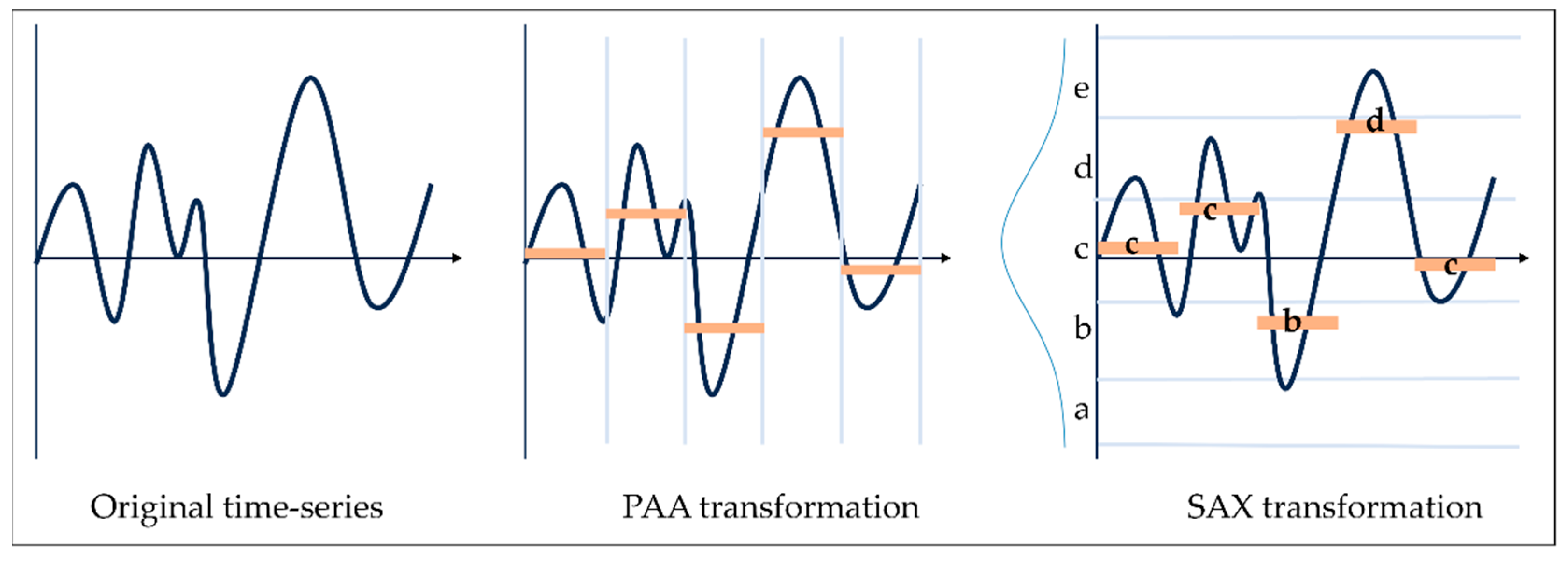
• We propose a new seasonal partition criterion using the SAX algorithm. By applying data smoothing techniques and SAX, we represent each data feature as SAX symbol patterns. The SAX algorithm serves two key purposes. First, it determines whether a feature is seasonal. Second, it obtains new seasonal criteria based on the SAX symbol patterns.
• We propose a two-layer stacked Long Short-Term Memory (LSTM) network to forecast power generation by partitioning data according to the new seasonal criteria. The optimal LSTM is trained for each newly defined season: spring, summer, autumn, and winter. Subsequently, the seasonal power generation forecasts are aggregated to derive a one-year forecast. The forecast values for one year obtained from each seasonal partition criterion are combined using averaging, weighted averaging, and stacking methods to produce the final forecast value.
• We evaluate the performance of the proposed method with the forecasting results of two real-world datasets; one from Gyeongju, South Korea, and one from California, USA. We compare the performance of a single LSTM without data partitioning, seasonal LSTMs with fixed seasonal partitions, and seasonal LSTMs with unfixed seasonal partitions. The results indicate that our method achieved the highest forecasting accuracy in terms of R-squared (R²), Root Mean Squared Error (RMSE), and Mean Absolute Error (MAE). Specifically, our method outperformed the others by 2.2% to 3.5%; and by 1.6% to 6.5% for the Gyeongju and California datasets, respectively.

The rest of this study is organized as follows: Section 2 reviews related studies, Section 3 introduces the proposed method, and Section 4 evaluates the performance of the proposed method. Finally, Section 5 concludes the study and determines future works.

2. Related Studies

In this section, we summarize the related studies in detail, under three categories: Methods for General Power Generation Forecasting, Methods for Power Generation Forecasting by Seasons, and Methods for Finding Unfixed Seasons.

2.1. Methods for General Power Generation Forecasting

A. Ozbek et al. [21] used LSTM, Adaptive Neuro-fuzzy Inference System (ANFIS), and ANFIS with grid partition to forecast one hour ahead of solar energy power generation. The experimental results conducted in the datasets from Mersin Province in southern Turkey revealed that the LSTM model provides the best RMSE and MAE of 60.66 and 30.47, respectively. Y. Li et al. [24] used the ARMAX model to forecast solar power generation. The proposed model used meteorological factors such as temperature, precipitation, sunlight, and humidity as exogenous variables. The experimental results showed that based on RMSE, Mean Absolute Deviation (MAD), and Mean Absolute Percentage Error (MAPE), the proposed method had higher performance than the Radial Basis Function (RBF) network model commonly used to predict power generation. M. Konstantinou et al. [25] conducted solar power generation forecasting using a stacked LSTM network. The authors excluded meteorological factors such as temperature, solar radiation, and relative humidity, and forecasted power generation using only past and current power generation, which are endogenous variables. As a result of the experiment, the proposed model predicted the fluctuations and trends of power generation well, and the RMSE was 0.11368. When the cross-validity method was applied, the average RMSE was 0.09394. M. Elsaraiti and A. Merabet [26] forecasted short-term solar power generation using the LSTM algorithm. The authors compared the proposed LSTM network with the Multi-Layer Perceptron (MLP) algorithm; a widely used technique in the literature. As a result of the comparison, the forecasting performance of the LSTM model was found to be excellent based on the evaluation metrics.

2.2. Methods for Power Generation Forecasting by Seasonal Partition

A. Gopi et al. [6] analyzed the impact of weather features to forecast solar power generation throughout the seasons. The dataset collected in Kerala, South India, is partitioned by seasons, such as Southwest monsoon (June to September), Northeast monsoon (October to November), Summer (February to May), and Winter (December to January). The authors could clarify the relation between solar power generation and weather features based on the seasonal partition analysis. Y. Hu et al. [7] forecasted solar power generation using a seasonal model based on a multilayer Backpropagation Neural Network (BPNN). Meteorological factors such as solar radiation, ambient temperature, and relative humidity were partitioned as the meteorological seasonal criteria. A multilayer BPNN with an optimal structure for each season was constructed. Experimental results showed that the proposed method was superior to the single-layer BPNN model and Support Vector Machine (SVM) regarding accuracy, RMSE, and MAE. F. Golestaneh et al. [8] conducted a study to forecast solar power generation using only power generation and weather information without sky images or cloud information. The authors propose partitioning the dataset by meteorological season and applying non-parametric probabilistic forecasting using the Extreme Learning Machine (ELM) model. As a result, the proposed method was proven to be stable and efficient in the very short term.

M. O. Moreira et al. [9] realized seasonal solar power generation forecasting using multivariate strategies based on the Design of Experiments (DOE), Principal Component Analysis (PCA), and Artificial Neural Network (ANN). The data are partitioned by season, and several climate variables are considered for each season. The minimum MAPE obtained with the proposed method was 6.75% in spring, 10.45% in summer, 9.29% in autumn, and 9.11% in winter. M. Elsaraiti et al. [26] forecasted solar power generation using LSTM and MLP in two seasonal partitions: winter and summer. The dataset used in the experiments was collected from Nova Scotia, Canada. The experimental results show that the LSTM model offered more effective performance than MLP in different seasons. T. Chuluunsaikhan et al. [27] studied the influence of data partition strategies to forecast solar power generation. The authors applied Window, Shuffle, Pyramid, Vertical, and Seasonal partition strategies to improve the performance of LSTM. Among the several data partition techniques, the result of seasonal data partition outperformed other strategies.

2.3. Methods for Finding Unfixed Seasons

J. Kwon and Y. Choi [12] used PCA and k-means clustering to define seasonal partition criteria by reflecting various climate factors and classifying synoptic patterns. As a result of the study, the start dates of the seasons were defined as 8 March, 6 June, 8 September, and 29 November, respectively. This study showed that seasons can vary depending on region and era. E. Lee et al. [13] introduced a data processing method to define each season’s indicators, such as start date, length, and abnormal days in South Korea. The daily mean temperatures of the past (1921 to 2010) and future (2021 to 2100) were used to estimate the three indicators. The authors defined detailed indicators that express seasonal partition by each administration region. Zhang. Z et al. [14] proposed the K-Means Time Series Clustering (K-MTSC) algorithm to cluster the intensity of solar radiation. As a result of the study, the start dates of the four seasons were newly defined as 10 May, 7 July, 10 November, and 28 January. The proposed method was improved over the astronomical seasonal standard in terms of average intra-cluster distance and average inter-cluster distance. This study showed that new seasonal criteria can define the four seasons according to the intensity of solar radiation.

3. Materials and Methods

3.1. Overview

Figure 1 illustrates the overall flow of the proposed method, which consists of data collection, data preprocessing, feature selection, seasonal criteria determination, data partitioning, seasonal modeling, ensemble, and evaluation steps. First, we collected power generation and weather data from a solar power plant in Gyeongju, South Korea [28], and one in California, USA [29]. Second, we performed preprocessing steps, including data cleaning and normalization. Third, we selected seasonal features from the dataset, excluding power generation, to establish seasonal partition criteria based on weather features. Fourth, the preprocessed data were partitioned according to these seasonal criteria. Fifth, we obtained forecasting results by training the optimal LSTM model for each new seasonal dataset. These results were then categorized according to each partition criterion. Finally, we evaluated the performance of the proposed method using R-squared, RMSE, and MAE as performance metrics. The subsequent subsections provide a detailed explanation of each step.

3.2. Data Collection

The first dataset used in the methodology is from a solar power plant in Gyeongju, South Korea [28]. This dataset includes hourly power generation data and weather features such as irradiation, dew point, temperature, humidity, and cloud cover. It consists of 17,532 hourly samples recorded over four years. The second dataset is the California data from Santa Barbara, California, USA, created by the National Renewable Energy Laboratory (NREL), Special Interest Groups Energy (SIG Energy), and the University of Massachusetts Amherst [29]. We use three-year data that includes 12,056 samples in 30 min intervals. It contains 11 power and weather features, such as Irradiance, Dew Point, Temperature, Humidity, Pressure, Precipitable Water, Wind Speed, Wind Direction, Surface Albedo, and Solar Zenith Angle. Detailed information about the datasets is provided in

Table 1. Details of datasets.

Dataset	Gyeongju	California
Number of features	6	11
Samples	17,532	12,056
Date	1 January 2017~31 December 2020	1 January 2014~31 December 2016
Time	00:00~23:00	10:00~15:00
Unit of time	1 h	30 min
Power capacity	1502.55 kWh	155 kWh

.

3.3. Data Preprocessing

3.3.1. Data Cleaning of Gyeongju Dataset

Since solar power generation occurs only when the sun is up, data from 0:00 to 23:00, excluding the hours from 7:00 to 18:00, were excluded from the Gyeongju dataset. For Power and Irradiance features with consecutive missing values exceeding a week, we replaced these values with the average values from the same day in other years. Afterward, the remaining missing values were imputed using linear interpolation.

Table 2. Features of Gyeongju dataset.

Dataset	Mean	Std Dev	Min	Max	Explanation
Power	489.71	382.08	0.00	1396.85	The power output of panels (kW)
Irradiance	297.04	244.07	0.00	975.00	The amount of radiation on the ground (W/m2)
Dew Point	6.83	12.14	−26.90	28.00	Dew Point (°C)
Temperature	16.10	10.14	−12.90	39.20	Outside temperature (°C)
Humidity	58.62	23.18	0.00	100.00	The concentration of water vapor present in the air (%)
Cloud Cover	3.09	3.97	0.00	10.00	Amount of cloud

presents the statistical information and feature explanations for the six features of the cleaned Gyeongju dataset.

3.3.2. Data Cleaning of California Dataset

Nominal features were excluded from the dataset, as their inclusion could deteriorate model performance. Since there were no missing values in the data, no further processing was required.

Table 3. Features of California dataset.

Dataset	Mean	Std Dev	Min	Max	Explanation
Power	49.82	17.60	1.10	76.31	The power output of panels (kW)
Irradiance	677.35	243.19	4.00	1074.00	The amount of radiation on the ground (W/m2)
Dew Point	7.85	4.05	−8.00	20.00	Dew point (°C)
Temperature	22.95	5.17	10.00	36.00	Outside temperature (°C).
Humidity	46.00	15.73	13.65	100.00	The concentration of water vapor present in the air (%)
Pressure	991.70	3.95	980.00	1010.00	Pressure (mbar)
Precipitable	1.63	0.76	0.21	5.68	Accumulated amount of water vapor contained in atmospheric space (mm)
Wind Speed	3.29	1.54	0.00	9.60	The speed of the wind within the atmosphere (m/s)
Wind Direction	247.52	71.66	0.00	359.90	Wind direction (degrees)
Surface Albedo	0.13	0.01	0.12	0.14	The fraction of solar radiation that is reflected by the surface of the Earth (degrees)
Solar Zenith Angle	41.47	15.69	11.01	72.74	the angle between the direct line to the sun and the location

presents the statistical information and feature explanations for the 11 features of the cleaned California dataset.

3.3.3. Data Normalization

During the data normalization step, Min-Max normalization is applied to the dataset. This process reduces data redundancy and prevents bias towards large-scale features. The formula for Min-Max normalization is shown in Equation (1).

$$x^{`}={\displaystyle \frac{x-x_{min}}{x_{max}-x_{min}}}$$

(1)

Here, expressions of the equation are explained as follows. $x^{`}$, $x$, $x_{min}$, and $x_{max}$ are normalized data, the original data, the minimum value of the dataset, and the maximum value of the dataset, respectively.

3.4. Seasonal Feature Selection

We designed a seasonal feature selection algorithm based on data smoothing and SAX techniques to determine whether a feature is seasonal. Algorithm 1 shows the pseudocode of this seasonal feature selection algorithm. Here, the input is the daily aggregated values of a feature and parameter configurations for data smoothing techniques. The algorithm returns the True/False value, indicating whether the feature is seasonal, and the parameter configuration for the selected data smoothing technique. The detailed steps of Algorithm 1 are explained as follows. The algorithm iterates through each data smoothing technique parameter option until the feature is considered as seasonal (Lines 2 to 12). First, it normalizes the feature data with and without smoothing (Lines 3 to 8). Second, the SAX transforms the normalized data (Line 9). Third, if the transformed data are considered seasonal, the algorithm terminates (Lines 10 to 12). Lastly, if the transformed data are not seasonal for all smoothing parameter options, the algorithm ends with False and None (Line 14). The detailed explanations of the steps are described in the following sub-sections.

Algorithm 1. SAX-based seasonal feature selection

Input       $X$: Feature data to check if it is a seasonal feature       $X_d$: Daily interval data where is aggregated over the same days       $pram$: An array containing options for the order of parameters in smoothing Output       $result$: Results of checking whether it is a seasonal feature       $p$: Final parameters of the smoothing method

1: $p$ ← $None$      2: for $i$ in range(0, length($pram$)):      3:   if $i$ == 0 then      4:      ${normalX}_d$ ← $Normalized\left(X_d\right)$      5:   else      6:      $p$ ← $pram[i-1]$      7:      $smoothed{X}_d$ ← $Smoothing(X_d,p)$      8:      $normal{X}_d$ ← $Normalized\left({smoothedX}_d\right)$      9:    $symbol{X}_d$ ← $SAX\left(normal{X}_d\right)$      10:  if $symbol{X}_d$ is Seasonal then      11:      $result$ ← True      12:      return $result,p$      13:    $result$ ← False      14: return $result,None$

3.4.1. Changing Data to Day-Interval

We aim to obtain a date criterion that can optimally capture seasonal changes. To achieve this, we convert the datasets to daily intervals to determine whether a feature is seasonal. For each day, the Power data is summed, and the weather features are averaged. Figure 2 compares the graphs of the Temperature feature before (Figure 2a) and after (Figure 2b) the daily interval conversion. As can be seen in the graph, converting to daily intervals reduces the number of data points, thereby simplifying the graph. Note that this conversion to daily intervals is intended for seasonal partitioning, not for forecasting.

3.4.2. Data Smoothing

When the normalized data of a feature are not identified as seasonal, we apply smoothing techniques such as Moving Average, Exponential Smoothing, or Gaussian Kernel Smoothing to the feature data. First, we select a set of parameters for each smoothing technique. We then smooth the feature data using each parameter until the data meet the conditions for being considered seasonal. If no parameter configuration results in the feature data being seasonal, the feature is deemed non-seasonal.

Moving Average is a method of smoothing data using the recent n average values as new values. Here, $n$ means the order of the Moving Average—the larger $n$ makes the data smoother. Equation (2) shows the formula for the Moving Average. Here, ${\overline{p}}_{MA}$, $p_0$, $p_{-\left(n-1\right)}$, $n$ are smoothed value, value at the current time, value at $n$ time ago, and order of Moving Average, respectively. We set $n$ to start from 10 and increase up to 100 by 10.

$${\overline{p}}_{MA}={\displaystyle \frac{p_0+p_{-1}+\dots +p_{-(n-1)}}{n}}$$

(2)

Exponential Smoothing is a method of performing smoothing by giving greater weight to recent data. The weight is determined according to the smoothing parameter $\alpha$. If $\alpha$ is small, a high weight is given to previous data. On the contrary, if $\alpha$ is large, high weight is given to recent data. Equation (3) shows the formula for Exponential Smoothing. Here, $L_{t+1}$, $\alpha$, $Y_{t+1}$, and $L_t$ are smoothed value, smoothing parameter between [0, 1], actual value at time $t+1$, smoothed value at time $t$. We set $\alpha$ to start from 0.1 to decrease up to 0.01 by 0.01.

$$L_{t+1}=\alpha Y_{t+1}+\left(1-\alpha \right)L_t$$

(3)

Gaussian Kernel Smoothing is a form of kernel smoothing, a non-parametric method that does not require prior data knowledge. It uses a Gaussian Kernel that follows a Gaussian distribution. The kernel assigns weights, and Gaussian Kernel Smoothing is especially useful when the amount of data is small, or the data are unbalanced. Equation (4) shows the formula of the Gaussian Kernel Smoothing method. Here, $f\left(x\right)$, $x$, $\mu$, and $\sigma$ are smoothed value, current value, mean, and standard deviation of the feature data.

$$f\left(x\right)={{\displaystyle \frac{1}{\sqrt{2\pi {\sigma }^2}}}e}^{-{\displaystyle \frac{{\left(x-\mu \right)}^2}{2{\sigma }^2}}}$$

(4)

Figure 3 shows an example of data smoothing methods. It presents the smoothed Temperature feature data from the Gyeongju dataset using various techniques with optimal parameters. As shown in Figure 3, Figure 3a shows the original Temperature values, and Figure 3b–d show smoothed values by Moving Average, Exponential Smoothing, and Gaussian Kernel, respectively. Data smoothing techniques reduce fluctuations and clarify the underlying trends in the data.

3.4.3. Assigning SAX Symbols

SAX is a technique that is commonly used for time series data for dimensionality reduction and data representation. It transforms continuous numerical values into discrete symbols. To that, SAX completes the four steps including Normalization, Piecewise Aggregate Approximation (PAA) transformation, SAX transformation, and Symbolic Representation. A detailed explanation of SAX is as follows, as shown in Figure 4. First, a time series data $C$ of length $n$ should be scaled in any normalization techniques like Min-Max or Standard scalers. In PAA transformation, the time series $C$ is divided into $w$ segments of equal size $n/w$, and the values included in each segment are averaged to obtain the corresponding PAA coefficient $\overline{\left(c_i\right)}$. Equation (5) represents the calculation formula for $\overline{\left(c_i\right)}$, the PAA coefficient of the $i$-th segment. Here, $\overline{\left(c_i\right)}$ represents PAA coefficient of $i$-th segment, and $c_k$ represents one point value in time series $C$.

$$\overline{c_i}={\displaystyle \frac{w}{n}}\sum _{k=\left({\displaystyle \frac{n}{w}}\right)\left(i+1\right)+1}^{\left({\displaystyle \frac{n}{w}}\right)i}{c}_k$$

(5)

In SAX transformation, an alphabet symbol is assigned to the PAA coefficients. At this time, the Gaussian distribution is divided into areas of equal size. Finally, when the symbol is sorted, an alphabet corresponding to the area is assigned to each segment. Figure 4 shows the PAA conversion and SAX conversion process by setting the time series to the number of segments $w=5$ and the symbol size $a=5$.

Figure 5 shows an example of assigning SAX symbols to Temperature values in the Gyeongju dataset using three smoothing techniques. First, original values are smoothed using Moving Average (Figure 5a), Exponential Smoothing (Figure 5b), and Gaussian Kernel Smoothing (Figure 5c) techniques. The smoothed data are then normalized. After that, we assigned three SAX symbols $a$ (a, b, c) at intervals of 10 segments, denoted as $w$. The parameter selection of $w=10$ and $a=3$ are chosen from several combinations to capture sufficient trends or patterns in the data. Specifically, the normalized values are approximately in the range of [–2, 2]. SAX divides this range into three equal intervals: [−2, −0.67), [−0.67, 0.67), and [0.67, 2]; each represented by the symbols a, b, and c, respectively. Each temperature value is assigned a symbol based on the interval it falls into. This symbol pattern effectively expresses seasonal changes in the Temperature data.

3.4.4. Determining Seasonal Features

In the proposed method, we apply the SAX technique to transform the time series data of each feature by year. Here, a feature is considered seasonal if the SAX symbols a, b, and c are formed in a consistent pattern, rather than occurring randomly across all years.

Example 1.

Consider the Temperature data for Gyeongju in the year 2017. The SAX transformation for this data results in the symbols: aaaaaaaaabbbccccccccccccccbbbaaaa. For the sake of simplicity, this sequence can be represented by continuous lowercase symbols as single capital symbols. Therefore, the sequence becomes (A, B, C, B, A), where:

• Continuous a symbols are represented as A
• Continuous b symbols are represented as B
• Continuous c symbols are represented as C

As shown in Figure 5a, the pattern (A, B, C, B, A) indicates that the Temperature feature in Gyeongju for 2017 follows a consistent seasonal pattern. In our dataset, we identified six consistent patterns that represent seasonality. A feature is considered seasonal if its SAX symbols follow one of these patterns: (A, B, C, B, A), (B, C, B, A), (A, B, C, B), (C, B, A, B, C), (B, A, B, C), and (C, B, A, B).

Table 4. Seasonal features identified using SAX technique.

Smoothing Technique	Features Identified in Gyeongju Dataset	Features Identified in California Dataset
Moving Average	Irradiance Dew Point Temperature	Irradiance Solar Zenith Angle Precipitable Temperature Pressure
Exponential Smoothing	Dew Point Temperature	Irradiance Solar Zenith Angle Pressure
Gaussian Kernel Smoothing	Irradiance Dew Point Temperature	Irradiance Solar Zenith Angle Precipitable Pressure

presents the seasonal features identified through each data smoothing technique. For example, Irradiance, Dew Point, and Temperature features are mainly determined as seasonal in the Gyeongju dataset. However, Irradiance is excluded in the case of the Exponential Smoothing technique. Irradiance, Solar Zenith Angle, and Pressure are the features that selected by all smoothing techniques in the California dataset. Additionally, the Moving Average technique identifies Precipitable and Temperature, and the Gaussian Kernel Smoothing technique identifies Precipitable. Each seasonal feature has its own symbol pattern for each year.

3.5. Seasonal Criteria and Data Partition

In the previous section, we identified that our seasonal features follow patterns: (A, B, C, B, A), (B, C, B, A), (A, B, C, B), (C, B, A, B, C), (B, A, B, C), and (C, B, A, B). Consequently, we also partition our datasets based on these patterns. We define unfixed seasonal criteria for each seasonal feature and each year separately, considering each data smoothing technique. This results in 68 different seasonal criteria for the two datasets. Specifically, the Gyeongju dataset has 32 seasonal partition criteria, calculated from 4 years × 8 seasonal features obtained using the three data smoothing techniques. In contrast, the California dataset has 36 seasonal partition criteria, derived from 3 years × 12 seasonal features.

Example 2.

Using the Temperature feature as an example, we demonstrate how SAX symbols are utilized to identify seasonal transitions and create unfixed seasonal partitions. As depicted in Figure 5a, the temperature feature follows the pattern (A, B, C, B, A), where: A, B, and C represent lower, middle, and higher temperatures, respectively. Each transition point (i.e., date) between SAX symbols represents a change in seasons. Using the temperature pattern (A, B, C, B, A), the partitioning for a specific year may look as follows:

• The transition point between A and B marks the start of spring
• The transition point between B and C marks the start of summer
• The transition point between C and B marks the start of autumn
• Winter starts on January 1st and at the transition point between B and A

Figure 6 illustrates the specific dates of season changes based on this unfixed partitioning method. Unlike meteorological and astronomical partitions, our unfixed partitions can capture precise seasonal changes based on the feature and year. Moreover, in the Performance Evaluation section, we will demonstrate that these unfixed seasonal partitions help the prediction models better understand the characteristics of the training data.

3.6. Training Ensemble LSTM Model

LSTM [30,31,32] is a particular type of Recurrent Neural Network (RNN) that can solve long-term dependence and gradient vanishing problems by implementing a gating mechanism. LSTM also has an internal recurrent structure like RNN. However, unlike RNN, LSTM has a complex hidden layer structure. Figure 7 shows the hidden layer structure of LSTM. It has three interactional layers, such as forgot gate, input gate, and output gate. In the LSTM process, the first step involves passing data through the input gate, where the decision is made about which information to store in the cell state. Simultaneously, the forget gate determines what information from the cell state should be discarded. In the next step, based on these decisions, unnecessary information is discarded, and new information is stored, updating the cell state. Finally, as the data pass through the output gate, the LSTM returns the final results based on the updated cell state. In this study, we utilize a two-layer stacked LSTM. The first LSTM layer processes the input sequence and outputs a sequence of hidden states. The second LSTM layer takes this sequence of hidden states and produces a final set of hidden states, which we use to predict solar power generation. This two-layer stacked LSTM structure can better capture and represent patterns in complex sequential data.

Figure 8 illustrates the process of the ensemble LSTM method to forecast solar power generation. We use training data partitioned into unfixed seasonal criteria based on each feature. After that, two-layer stacked LSTMs, which have a structure of two layers, learn data for each season separately. All results from each seasonal partition are merged and ensembled by several methods, such as average, weighted average, and stacked. The average method takes the average value of all forecasting results. The weighted average method takes the average value while considering the accuracy of each forecasting result. Here, we use the reciprocal of RMSE as weight because smaller RMSE values indicate higher accuracy. For the stacked method, we train a Linear Regression method that learns the forecasting results to return new optimal results.

4. Performance Evaluation

4.1. Datasets

In the experiments, we utilized fixed and unfixed seasonal partitioned datasets from Gyeongju, South Korea; and California, USA. The Gyeongju dataset was available for four years between 2017 and 2020. The California dataset was available for three years between 2014 and 2016. The training dataset is selected from all years, excluding the last year. The last year of each dataset is used for evaluating prediction models as testing data.

Table 5. Train/Test data split.

	Gyeongju	California
Training data	2017–2019	2014–2015
Test data	2020	2016

shows the Train/Test data splitting of the Gyeongju and California datasets.

4.2. Evaluation Metrics

R², RMSE, and MAE were used as indicators to evaluate performance. R² is an indicator of relative performance, and the closer it is to 1, the higher the performance. Unlike other indicators, it is easy to compare multiple cases. RMSE is a value rooted at the Mean Squared Error, the average of the squared difference between the actual and predicted values. The smaller the value, the higher the performance. MAE is the average value of the absolute value of the difference between the actual value and the predicted value. The smaller the value, the higher the performance. The equation for each indicator is (6), (7), and (8). Here, $n$, $y_i$, $\widehat{y_i}$, and $\overline{y_i}$ are the number of test samples, an actual value, a predicted value, and the mean of actual values, respectively.

$$R^2={\displaystyle \frac{{\sum }_{i=1}^n{\left(y_i-{\widehat{y}}_i\right)}^2}{{\sum }_{i=1}^n{\left(y_i-{\overline{y}}_i\right)}^2}}$$

(6)

$$RMSE=\sqrt{{\displaystyle \frac{{\sum }_{i=1}^n{\left(y_i-{\widehat{y}}_i\right)}^2}{n}}}$$

(7)

$$MAE={\displaystyle \frac{1}{n}}\sum _{i=1}^n|y_i-{\widehat{y}}_i|$$

(8)

4.3. Competing Methods

We proposed a new SAX-based unfixed seasonal partition approach using the LSTM model. To compare our method with general and seasonal partition forecasting methods, we conducted a comparative experiment using a general LSTM model and seasonal models based on two commonly used seasonal criteria.

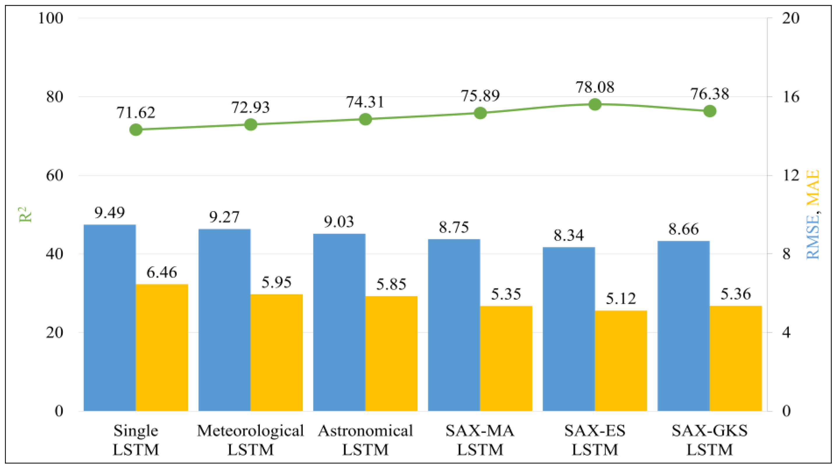
• Single LSTM: This is a method to forecast solar power generation by training an optimal LSTM on the entire dataset, without any data partition.
• Meteorological LSTM: This method divides the data by a fixed season according to the most commonly used criteria, called meteorological: spring, March to May; summer, June to August; autumn, September to November; and winter, December to February. Afterward, the optimal LSTM is trained for each divided data to forecast power generation.
• Astronomical LSTM: This is a method of dividing fixed seasons according to the sun’s position on the celestial sphere astronomically. First, divide the data according to the astronomical seasons. Spring is from 22 March to 21 June, summer is from 22 June to 22 September, autumn is from 23 September to 21 December, and winter is from 22 December to 22 March. Then, the optimal LSTM is trained for each divided data to forecast power generation.
• SAX-MA LSTM: Method using the unfixed seasonal partition based on SAX and the Moving Average smoothing technique.
• SAX-ES LSTM: Method using the unfixed seasonal partition based on SAX and the Exponential Smoothing technique.
• SAX-GKS LSTM: Method using the unfixed seasonal partition based on SAX and the Gaussian Kernel Smoothing technique.

Table 6. Parameter options and descriptions of LSTM.

Parameter	Options	Description
batch_size	64, 128	Number of data samples processed by a model in one training iteration.
epochs	1000	Total number of dataset iterations
patience	10	The number of epochs used in early stop
learning_rate	0.01, 0.001	Learning rate in gradient descent
layers	2	Number of layers
units	32, 64, 128, 256	Number of units in each layer
optimizer	Adam	Optimizer
loss_function	MSE	Loss function

shows the parameter options and descriptions used in our experiments. The same parameter options for LSTM model construction were used as candidate parameters in all experiments. We train the LSTM model with all possible combinations and compare the accuracy based on R². A combination that ensured optimal accuracy based on R² was used in all experiments. The remaining experimental environment was also conducted in the same manner as the method proposed in this paper. We also applied Early Stopping with a patience of 10 to address overfitting.

4.4. Experimental Results

4.4.1. Results for Comparing Competing Methods

Figure 9 illustrates the comparison of experimental results for the Gyeongju dataset. The green line represents R², and the blue and yellow bars represent RMSE and MAE, respectively. In this experiment, we compared the non-partitioning (Single LSTM), fixed seasonal partitioning (Meteorological and Astronomical LSTMs), and unfixed seasonal partitioning (SAX-MA, SAX-ES, and SAX-GKS LSTMs) based on three data smoothing techniques and SAX. The experimental results demonstrate that our proposed unfixed seasonal partition methods outperformed non-partitioned and fixed seasonal partitioned predictions across all evaluation metrics. The results show that fixed seasonal partitioning helps improve the performance of non-partitioned forecasting solar power generation by about 1.2% in terms of R². Moreover, we improved the R² score by 3.5% with a more specific unfixed seasonal partition. Our proposed method also shows lower RMSE and MAE scores than non-partitioned and fixed partitioning forecasts.

Figure 10 illustrates the comparison of experimental results for the California dataset. The experimental results are similar in pattern to those obtained with the Gyeongju dataset. Specifically, fixed partitioning methods outperformed the non-partitioned method by 2.7%, and our unfixed partitioning methods outperformed the non-partitioned method by 6.4% in terms of R². Our proposed method also shows lower RMSE and MAE scores than non-partitioned and fixed partitioning forecasts.

Based on the results shown in Figure 9 and Figure 10, seasonal partitioning is important to forecast solar panel power generation. Because data in each season have similar characteristics, they help prediction models achieve more robust and accurate performance. Our proposed method identifies the precise dates of seasonal partitioning, making the prediction models more learnable.

4.4.2. Results for Ensemble Effects

Table 7. Single and Ensemble forecast results of Gyeongju dataset.

Method		R2	RMSE	MAE
SAX-MA LSTM	Based on Irradiation	85.65%	145.76	101.69
	Based on Dew Point	86.51%	141.3	99.52
	Based on Temperature	86.13%	143.3	100.14
	Average Ensemble	87.87%	133.71	90.95
	Weighted Ensemble	87.87%	133.97	92.3
	Stacking Ensemble	87.92%	133.71	90.95
SAX-ES LSTM	Based on Dew Point	86.04%	143.75	100.75
	Based on Temperature	86.66%	140.52	95.6
	Average Ensemble	87.91%	133.77	92.37
	Weighted Ensemble	87.91%	133.75	92.34
	Stacking Ensemble	88.04%	133.04	90.22
SAX-GKS LSTM	Based on Irradiation	86.75%	140.02	98.99
	Based on Dew Point	85.74%	145.31	99.56
	Based on Temperature	86.34%	142.17	96.56
	Average Ensemble	88.00%	133.25	92.21
	Weighted Ensemble	88.01%	133.21	92.2
	Stacking Ensemble	88.12%	132.62	91.24

presents the experimental results for unfixed seasonal partitions in the Gyeongju dataset, both with and without the ensemble learning module. We compare the performance metrics for data smoothing techniques and seasonal features, including R², RMSE, and MAE. Subsequently, we compare the ensemble results using three different methods. Overall, all ensemble methods demonstrate an improvement in R² by approximately 1% to 2%. More specifically, the stacking ensemble outperforms other methods in all experimental cases.

Table 8. Single and Ensemble forecast results of California dataset.

Method		R2	RMSE	MAE
SAX-MA LSTM	Based on Irradiation	73.12%	9.24	5.8
	Based on Temperature	71.22%	9.56	6.1
	Based on Pressure	72.72%	9.48	6.1
	Based on Precipitable	68.86%	9.95	6.65
	Based on SZ Angle	73.87%	9.11	5.74
	Average Ensemble	75.51%	8.82	5.4
	Weighted Ensemble	75.54%	8.82	5.39
	Stacking Ensemble	75.89%	8.75	5.35
SAX-ES LSTM	Based on Irradiation	75.83%	8.76	5.52
	Based on Pressure	75.75%	8.78	5.53
	Based on SZ Angle	73.87%	9.11	5.74
	Average Ensemble	77.86%	8.39	5.13
	Weighted Ensemble	77.88%	8.38	5.13
	Stacking Ensemble	78.08%	8.34	5.12
SAX-GKS LSTM	Based on Irradiation	73.68%	9.14	5.83
	Based on Pressure	74.63%	8.98	5.89
	Based on Precipitable	72.81%	9.29	6.09
	Based on SZ Angle	73.87%	9.11	5.74
	Average Ensemble	76.26%	8.68	5.31
	Weighted Ensemble	76.26%	8.68	5.31
	Stacking Ensemble	76.38%	8.66	5.36

presents the experimental results for unfixed seasonal partitions in the California dataset, both with and without ensemble. Like the Gyeongju dataset, the stacking ensemble method outperforms other methods in smoothing and ensemble data. There is one case that has lower RMSE and higher MAE in the stacking ensemble method of the Gaussian Kernel Smoothing. The case occurs when there are a few large errors in the forecasting because RMSE is sensitive to these large errors.

4.4.3. Results for Recent Methods with Unfixed Data Partition

In this paper, we implemented a two-layer stacked LSTM due to its advantages, including its ability to capture long-term patterns and complex relationships. The previous experimental results showed that the proposed unfixed seasonal partitioning method improved forecasting performance compared to non-partitioned and fixed-partitioned data. Therefore, we also evaluated the effects of unfixed data partitioning on recent time series forecasting methods to demonstrate that the proposed approach can be applied not only to LSTM models but also to other forecasting models. We selected Temporal Convolutional Network (TCN) [33,34,35] and InceptionTime [36,37,38].

• TCN is a type of neural network designed to handle sequence data (i.e., time series) using convolutions to learn patterns over time. It captures long-term dependencies efficiently and avoids the problems of LSTM including slow training and vanishing/exploding gradients.
• InceptionTime is a deep learning method that adapts the Inception architecture from image processing. It uses different sized filters to capture patterns in time series sequences. By processing multiple patterns at once, it learns complex time series data quickly and effectively.

Table 9. Effects of unfixed data partition on recent time series forecasting methods.

Dataset	Method	TCN			InceptionTime
		R2	RMSE	MAE	R2	RMSE	MAE
Gyeongju	Non-partitioned	81.35%	166.13	116.23	68.67%	215.32	164.78
	Meteorological	82.73%	159.86	111.26	75.53%	190.31	140.16
	Astronomical	83.15%	157.91	111.19	73.27%	198.89	154.37
	SAX-MA	84.89%	149.53	105.77	80.64%	169.28	125.85
	SAX-ES	85.27%	147.64	101.84	79.61%	173.73	126.84
	SAX-GKS	84.91%	149.46	101.81	81.04%	167.51	114.42
California	Non-partitioned	64.06%	10.69	7.34	62.99%	10.84	8.26
	Meteorological	68.12%	10.06	6.66	60.20%	11.24	8.23
	Astronomical	69.76%	9.80	6.65	62.44%	10.92	8.27
	SAX-MA	70.36%	9.70	6.22	64.34%	7.73	7.73
	SAX-ES	70.06%	9.75	6.84	67.09%	7.16	7.16
	SAX-GKS	70.80%	9.63	6.33	64.41%	10.63	8.00

presents the forecasting results of the two methods on non-partitioned, fixed-partitioned, and proposed unfixed-partitioned datasets. For the Gyeongju dataset, we used the unfixed partitioned dataset based on temperature feature. The table shows that our proposed approach outperformed non-partitioned and fixed-partitioned in both the TCN and InceptionTime methods. Specifically, TCN improves the performance by 1.7% to 3.9%, while InceptionTime improves performance by 4% to 12.4% in terms of R² score. Additionally, for the California dataset (based on irradiation feature), our proposed method also improves performance by 0.3% to 6.9% in terms of R² score. Although both methods with unfixed partitioning show improved performance, our proposed two-layer stacked LSTM outperforms TCN and InceptionTime.

5. Conclusions

In this paper, we proposed a novel method to forecast solar panel power generation using unfixed seasonal data partition based on SAX and the ensemble LSTM method. For this purpose, we first partitioned the datasets based on unfixed seasonal criteria obtained by data smoothing techniques and SAX. Second, we train the two-layer stacked LSTMs for each criterion and ensemble the results using three popular methods. The experimental results showed that our proposed method improves the performance of non-partitioned and fixed-partitioned forecasting methods.

This paper aims to define new appropriate seasons according to data and focus on forecasting power generation for each new season. We obtained proper seasons through data analysis and performed new seasonal power generation forecasts. Our paper had three differences compared to existing studies. First, our method can select seasonal features among several features and divide seasons according to those features. Second, we perform seasonal power generation forecasts according to the seasonal partition criteria obtained based on each seasonal feature and ensemble all forecast results derived for each seasonal feature. Third, we demonstrated performance improvement by comparing the new seasonal power generation forecasting method based on our proposed method with the existing general seasonal power generation forecasting method.

Our findings in this study suggest that unfixed seasonal data partitions help obtain more precise characteristics of seasons than traditional fixed partitions, such as metrological and astronomical. Our proposed method can determine more specific points (i.e., dates) for finding seasonal changes based on solar power generation and weather features in any location. It helps to improve forecasting performance not only in the solar panel sector but also in other areas influenced by seasonal variations, such as agriculture, tourism, environmental monitoring, and more.

In the future, many studies may be conducted to improve the ideas proposed in this paper. Specifically, future work may explore data augmentation methods to further enhance model performance and address the limitations of the small dataset used in our experiments. Therefore, our method divides the data into four seasons per year. In the future, we can perform seasonal partition in more detail (i.e., three or six seasons).

References

1. Kosis Korean Statistical Information Service. Available online: https://kosis.kr/eng/ (accessed on 29 July 2024).
2. Doddy Clarke, E.; Sweeney, C. Solar Energy and weather. Weather 2021, 77, 90–91. [Google Scholar] [CrossRef]
3. Gopi, A.; Sharma, P.; Sudhakar, K.; Ngui, W.K.; Kirpichnikova, I.; Cuce, E. Weather impact on solar farm performance: A comparative analysis of machine learning techniques. Sustainability 2022, 15, 439. [Google Scholar] [CrossRef]
4. Ramirez-Vergara, J.; Bosman, L.B.; Leon-Salas, W.D.; Wollega, E. Predicting on-site solar energy generation using off-site weather stations and deep neural networks. Int. J. Energy Environ. Eng. 2022, 14, 1–13. [Google Scholar] [CrossRef]
5. Lim, S.-C.; Huh, J.-H.; Hong, S.-H.; Park, C.-Y.; Kim, J.-C. Solar Power Forecasting using CNN-LSTM hybrid model. Energies 2022, 15, 8233. [Google Scholar] [CrossRef]
6. Gopi, A.; Sudhakar, K.; Keng, N.W.; Krishnan, A.R.; Priya, S.S. Performance modeling of the weather impact on a utility-scale PV power plant in a tropical region. Int. J. Photoenergy 2021, 2021, 5551014. [Google Scholar] [CrossRef]
7. Hu, Y.; Lian, W.; Han, Y.; Dai, S.; Zhu, H. A seasonal model using optimized multi-layer neural networks to forecast power output of PV plants. Energies 2018, 11, 326. [Google Scholar] [CrossRef]
8. Golestaneh, F.; Pinson, P.; Gooi, H.B. Very short-term nonparametric probabilistic forecasting of renewable energy generation—With application to Solar Energy. IEEE Trans. Power Syst. 2016, 31, 3850–3863. [Google Scholar] [CrossRef]
9. Moreira, M.O.; Kaizer, B.M.; Ohishi, T.; Bonatto, B.D.; Zambroni de Souza, A.C.; Balestrassi, P.P. Multivariate strategy using artificial neural networks for seasonal photovoltaic generation forecasting. Energies 2022, 16, 369. [Google Scholar] [CrossRef]
10. Adusei, K.K.; Ng, K.T.; Mahmud, T.S.; Karimi, N.; Lakhan, C. Exploring the use of astronomical seasons in municipal solid waste disposal rates modeling. Sustain. Cities Soc. 2022, 86, 104115. [Google Scholar] [CrossRef]
11. Kutta, E.; Hubbart, J.A. Reconsidering meteorological seasons in a changing climate. Clim. Chang. 2016, 137, 511–524. [Google Scholar] [CrossRef]
12. Kwon, J.; Choi, Y. Application of synoptic patterns to the definition of seasons in the Republic of Korea. Int. J. Climatol. 2023, 43, 6268–6284. [Google Scholar] [CrossRef]
13. Lee, E.; Im, A.; Oh, J.; Song, M.; Choi, Y.; Choi, D. Improved seasonal definition and projected future seasons in South Korea. Meteorol. Appl. 2022, 29, e2110. [Google Scholar] [CrossRef]
14. Zhang, Z.; Wang, C.; Peng, X.; Qin, H.; Lv, H.; Fu, J.; Wang, H. Solar radiation intensity probabilistic forecasting based on K-means time series clustering and gaussian process regression. IEEE Access 2021, 9, 89079–89092. [Google Scholar] [CrossRef]
15. Lin, J.; Keogh, E.; Lonardi, S.; Chiu, B. A symbolic representation of time series, with implications for streaming algorithms. In Proceedings of the 8th ACM SIGMOD Workshop on Research Issues in Data Mining and Knowledge Discovery, San Diego, CA, USA, 13 June 2003. [Google Scholar] [CrossRef]
16. Wang, Z.; Wang, L.; Huang, C.; Zhang, Z.; Luo, X. Soil-moisture-sensor-based automated soil water content cycle classification with a hybrid symbolic aggregate approximation algorithm. IEEE Internet Things J. 2021, 8, 14003–14012. [Google Scholar] [CrossRef]
17. Jung, W.-K.; Kim, H.; Park, Y.-C.; Lee, J.-W.; Ahn, S.-H. Smart sewing work measurement system using IOT-based power monitoring device and approximation algorithm. Int. J. Prod. Res. 2019, 58, 6202–6216. [Google Scholar] [CrossRef]
18. Chiosa, R.; Piscitelli, M.S.; Capozzoli, A. A data analytics-based Energy Information System (EIS) tool to perform meter-level anomaly detection and diagnosis in buildings. Energies 2021, 14, 237. [Google Scholar] [CrossRef]
19. Ruan, H.; Hu, X.; Xiao, J.; Zhang, G. TrSAX—An improved time series symbolic representation for classification. ISA Trans. 2020, 100, 387–395. [Google Scholar] [CrossRef]
20. Bai, B.; Li, G.; Wang, S.; Wu, Z.; Yan, W. Time Series classification based on multi-feature dictionary representation and Ensemble Learning. Expert Syst. Appl. 2021, 169, 114162. [Google Scholar] [CrossRef]
21. Ozbek, A.; Yildirim, A.; Bilgili, M. Deep Learning Approach for one-hour ahead forecasting of energy production in a solar-PV plant. Energy Sources Part A 2021, 44, 10465–10480. [Google Scholar] [CrossRef]
22. Dhaked, D.K.; Dadhich, S.; Birla, D. Power output forecasting of Solar Photovoltaic Plant Using LSTM. Green Energy Intell. Transp. 2023, 2, 100113. [Google Scholar] [CrossRef]
23. Hossain, M.S.; Mahmood, H. Short-term photovoltaic power forecasting using an LSTM neural network and synthetic weather forecast. IEEE Access 2020, 8, 172524–172533. [Google Scholar] [CrossRef]
24. Li, Y.; Su, Y.; Shu, L. An ARMAX model for forecasting the power output of a grid connected photovoltaic system. Renew. Energy 2014, 66, 78–89. [Google Scholar] [CrossRef]
25. Konstantinou, M.; Peratikou, S.; Charalambides, A.G. Solar photovoltaic forecasting of power output using LSTM Networks. Atmosphere 2021, 12, 124. [Google Scholar] [CrossRef]
26. Elsaraiti, M.; Merabet, A. Solar power forecasting using Deep Learning Techniques. IEEE Access 2022, 10, 31692–31698. [Google Scholar] [CrossRef]
27. Chuluunsaikhan, T.; Kim, J.-H.; Shin, Y.; Choi, S.; Nasridinov, A. Feasibility Study on the influence of data partition strategies on Ensemble Deep Learning: The case of forecasting power generation in South Korea. Energies 2022, 15, 7482. [Google Scholar] [CrossRef]
28. Daeyeon C&I Co., Ltd. Available online: http://dycni.com/ (accessed on 29 July 2024).
29. Sauter, E. “Modeling PV Power On 6yrs Spatiotemporal Data,” GitHub. Available online: https://github.com/EvanSauter/Modeling-PV-Power-On-6yrs-Spatiotemporal-Data (accessed on 29 July 2024).
30. Hochreiter, S.; Schmidhuber, J. Long short-term memory. Neural Comput. 1997, 9, 1735–1780. [Google Scholar] [CrossRef]
31. Sansine, V.; Ortega, P.; Hissel, D.; Ferrucci, F. Hybrid Deep Learning Model for Mean Hourly Irradiance Probabilistic Forecasting. Atmosphere 2023, 14, 1192. [Google Scholar] [CrossRef]
32. Meng, H.; Wu, L.; Li, H.; Song, Y. Construction and Research of Ultra-Short Term Prediction Model of Solar Short Wave Irradiance Suitable for Qinghai–Tibet Plateau. Atmosphere 2023, 14, 1150. [Google Scholar] [CrossRef]
33. Shaojie, B.; Zico, J.; Vladlen, K. An Empirical Evaluation of Generic Convolutional and Recurrent Networks for Sequence Modeling. arXiv 2018, arXiv:1803.01271. [Google Scholar]
34. Wang, Y.; Zhang, C.; Fu, Y.; Suo, L.; Song, S.; Peng, T.; Shahzad Nazir, M. Hybrid solar radiation forecasting model with temporal convolutional network using data decomposition and improved artificial ecosystem-based optimization algorithm. Energy 2023, 280, 128171. [Google Scholar] [CrossRef]
35. Perera, M.; De Hoog, J.; Bandara, K.; Senanayake, D.; Halgamuge, S. Day-ahead regional solar power forecasting with hierarchical temporal convolutional neural networks using historical power generation and weather data. Appl. Energy 2024, 361, 122971. [Google Scholar] [CrossRef]
36. Ismail Fawaz, H.; Lucas, B.; Forestier, G.; Pelletier, C.; Schmidt, D.F.; Weber, J.; Webb, G.I.; Idoumghar, L.; Muller, P.-A.; Petitjean, F. InceptionTime: Finding alexnet for Time Series classification. Data Min. Knowl. Discov. 2020, 34, 1936–1962. [Google Scholar] [CrossRef]
37. Li, Y.; Yang, C. Multi Time Scale Inception-time network for soft sensor of blast furnace ironmaking process. J. Process Control. 2022, 118, 106–114. [Google Scholar] [CrossRef]
38. Putkonen, J.; Ahajjam, M.A.; Pasch, T.; Chance, R. A hybrid VMD-wt-InceptionTime model for multi-horizon short-term air temperature forecasting in Alaska. In Proceedings of the EGU23, the 25th EGU General Assembly, Vienna, Austria, 23–28 April 2023. [Google Scholar]
Figure 1. Overview of the proposed methodology. The symbols a–c represent the division of the data into equal sized areas or bins.
Electronics 13 03871 g001
Figure 2. Temperature of the Gyeongju dataset in hourly and daily intervals.
Electronics 13 03871 g002
Figure 3. Example of smoothed data by Temperature in Gyeongju dataset.
Electronics 13 03871 g003
Figure 4. PAA transformation and SAX transformation process. The symbols a–e are represent the division of the data into equal sized areas or bins.
Electronics 13 03871 g004
Figure 5. Assigning SAX symbols to temperature data in Gyeongju dataset. The symbols a–c represent the division of the data into equal sized areas or bins.
Electronics 13 03871 g005
Figure 6. Example of unfixed seasonal partition based on Temperature feature of the Gyeongju dataset.
Electronics 13 03871 g006
Figure 7. Hidden layer structure of LSTM.
Electronics 13 03871 g007
Figure 8. Seasonal solar power generation forecasting by ensemble LSTM method.
Electronics 13 03871 g008
Figure 9. Comparison experimental results of the Gyeongju dataset.
Electronics 13 03871 g009
Figure 10. Comparison of experimental results of the California dataset.
Electronics 13 03871 g010