Natural Language Inference with Transformer Ensembles and Explainability Techniques

Abstract

Natural language inference (NLI) is a fundamental and quite challenging task in natural language processing, requiring efficient methods that are able to determine whether given hypotheses derive from given premises. In this paper, we apply explainability techniques to natural-language-inference methods as a means to illustrate the decision-making procedure of its methods. First, we investigate the performance and generalization capabilities of several transformer-based models, including BERT, ALBERT, RoBERTa, and DeBERTa, across widely used datasets like SNLI, GLUE Benchmark, and ANLI. Then, we employ stacking-ensemble techniques to leverage the strengths of multiple models and improve inference performance. Experimental results demonstrate significant improvements of the ensemble models in inference tasks, highlighting the effectiveness of stacking. Specifically, our best-performing ensemble models surpassed the best-performing individual transformer by 5.31% in accuracy on MNLI-m and MNLI-mm tasks. After that, we implement LIME and SHAP explainability techniques to shed light on the decision-making of the transformer models, indicating how specific words and contextual information are utilized in the transformer inferences procedures. The results indicate that the model properly leverages contextual information and individual words to make decisions but, in some cases, find difficulties in inference scenarios with metaphorical connections which require deeper inferential reasoning.

1. Introduction

Natural language inference (NLI) is an important part of natural language processing. In general, it requires a method to determine whether or not a given hypothesis derives from a given premise. The first statement, known as the premise, provides the contextual foundation, while the second statement, the hypothesis, tests whether this context supports a particular inference. In NLI, “Entailment” means that the hypothesis logically follows from the premise. “Contradiction” indicates that the hypothesis logically contradicts the premise. “Neutral” signifies that the hypothesis and the premise are unrelated, or that the truth of the hypothesis cannot be determined based on the premise. Inherently, this process requires an understanding of context, since the relation between the premise and the hypothesis may widely differ due to subtle contextual cues [1,2].

Despite the apparent simplicity of matching a hypothesis to a premise, NLI is intrinsically complex due to the subtleties of natural language, including ambiguity, idiomatic expressions, and the need for common-sense reasoning. As human language is inherently imprecise and context-dependent, NLI tasks challenge models to navigate a wide range of linguistic variations, from direct assertions to nuanced implications. Consequently, achieving a robust and generalizable performance in NLI remains a critical and ongoing challenge in NLP research [3]. For example, consider the premise “The man is cooking” and the hypothesis “The man is a chef”. Depending on the context, this pair might be classified differently. If the man cooks professionally, the hypothesis would likely entail the premise. However, if the man is merely cooking as a hobby, the hypothesis would not necessarily follow. In cases where no additional information about the man’s occupation is provided, the relationship remains indeterminate. Determining the precise relationship between sentences can be difficult because natural language is frequently imprecise and context-dependent [3]. A background or common-sense knowledge that is not given clearly in the text is often necessary to understand entailment [4]. Additionally, recognizing paraphrases and variations of the same concept is essential for accurate NLI. For instance, “The dog is on the table” and “The table has a dog on it” convey the same idea but require the system to identify them as equivalent expressions. This fundamental complexity and variety of human language make NLI a quite challenging task [5,6].

To address these challenges, recent research has increasingly focused on the development of sophisticated models that leverage the power of large-scale pre-trained transformers [7]. These models, such as BERT, RoBERTa, and DeBERTa, have demonstrated significant improvements in NLI tasks by capturing intricate patterns in language through deep contextual embeddings [8]. However, while these models excel in many scenarios, they often struggle with specific cases requiring more complex reasoning, such as those involving figurative language or knowledge beyond the text. Moreover, the black-box nature of these models has raised concerns about their interpretability, especially in applications where understanding the rationale behind a decision is as crucial as the decision itself. This has led to the growing importance of explainability techniques in NLP, which aim to make the decision-making processes of these models more transparent and understandable to users and researchers alike. By integrating explainability methods with high-performance models, researchers hope to develop systems that are not only accurate but also reliable and interpretable, paving the way for more trustworthy AI applications in sensitive domains.

In this paper, we design ensemble transformer schemas for accurately performing natural language inference, and we utilize explainability techniques to illustrate the decision-making procedure of the transformers. First, we investigate the performance and generalization capabilities of several transformer-based models, including BERT, ALBERT, RoBERTa, and DeBERTa, across major datasets like SNLI, GLUE Benchmark, and ANLI. We employ stacking-ensemble techniques, leveraging the strengths of multiple models to improve inference performance. Experimental results demonstrate significant improvements of the ensemble models in natural-language-inference tasks, highlighting the effectiveness of ensembling approaches. Specifically, our best-performing ensemble model surpassed the best-performing individual transformer (T5) by 5.31% in accuracy on MNLI-m and MNLI-mm tasks. After that, we apply LIME and SHAP explainability techniques to shed light on the decision-making of the transformer models indicating how specific words and contextual information are utilized in the transformer inferences procedures. The results indicate that the model properly leverages contextual information and individual words to make decisions but, in some cases, finds difficulty in inference scenarios with metaphorical connections that require deeper inferential reasoning.

The rest of the article is structured as follows: Section 2 details the methods and models employed in this research and explains the ensemble models designed. Section 3 presents experimental results, demonstrating the performance improvements achieved through our proposed methods. Section 4 presents the explainability methods applied on the transformers and how they provide valuable information about the way they utilize words and contextual information in their inference procedure. Finally, Section 5 provides conclusions and discusses future research directions.

2. Related Works

A novel way to enhance natural language inference (NLI) is presented in the work in [9] which involves pre-trained language models (PLMs) like RoBERTa along with dynamic integration of external knowledge from multiple knowledge graphs (KGs) like WordNet and ConceptNet. For each input word, the suggested model generates a knowledge-enhanced graph, which is then processed using parallel graph neural networks (GNNs). By integrating intermediate results dynamically and synchronizing with the input text, these GNNs improve the model’s capacity to fill in the logical and semantic gaps between premises and hypotheses. The model has been evaluated using the SNLI, MNLI, and SciTail datasets and delivers state-of-the-art results with significant enhancements over previous models.

The work presented in [10] offers an extensive overview of the present state of natural language inference (NLI) datasets, identifies resource shortfalls, and suggests two new benchmarks to close these gaps. The lack of datasets concentrating on syntactically intricate, technically valid inferences and direct inductive inferences is noted by the authors. To address them, they present a novel syllogistic logic-based dataset that confronts models with formally valid inferences, as well as a dataset built from argumentative literature that stresses inductive reasoning. The research assesses cutting-edge transformer-based models on these novel datasets, such as ChatGPT, a finetuned DistillBERT (base-uncased), and others. It finds substantial difficulties in generalization, especially when dealing with neutral labels. According to the findings, models that have been fine-tuned on traditional datasets have difficulty with the various kinds of inference, while fine-tuning on newer datasets enhances performance at the expense of accuracy when compared to more established benchmarks. Further demanding and diverse NLI datasets are needed to improve model performance and generalization, as this research highlights.

The results of SemEval-2023 Task 7 are presented in this publication [11]. The task consisted of two primary challenges: an evidence selection task and a natural language inference (NLI) task. For the NLI task, models have to use complex multi-hop reasoning and numerical inference to classify a relationship between a statement and a clinical trial report (CTR) premise as either an entailment or a contradiction. Finding pertinent CTR passages that support the classifications stated in the NLI task was the goal of the evidence selection task. The NLI problem was especially difficult since it involved a lot of complex reasoning, including the integration of data from several CTR sections and the use of quantitative reasoning. Therefore, in the entailment task, several systems failed to surpass the majority-class baseline, demonstrating the difficulty of developing models that are capable of complicated inferencing in the biomedical domain. The findings showed that, in comparison to specialized biological pre-training, increasing model size greatly improves performance in these kinds of tasks. The work also highlights the fundamental obstacle for future research, which is how hard it is to generalize NLI models to new data without significantly sacrificing performance. Numerous strategies were investigated; in the entailment task, larger generative models typically outperformed others, but discriminative models were more successful in identifying evidence. The study comes to the conclusion that even while significant progress has been made, there is still much space for growth, especially when it comes to boosting numerical reasoning skills and making sure models can successfully generalize fresh data.

A thorough assessment of several deep-learning models for the task of natural language inference (NLI) is presented in the work in [12]. The authors, using eight well-known NLI datasets, analyze a total of five deep-learning models, including more contemporary transformer-based models like BERT, RoBERTa, and ALBERT and more conventional models like DAM and ESIM. The outcomes demonstrate the superiority of transformer-based models, especially ALBERT and RoBERTa, which on many datasets demonstrated state-of-the-art performance. Though these models perform well on individual datasets, the study also highlights the difficulties these models encounter when trying to generalize across other NLI datasets. The study shows that while transformer models show good NLI capabilities, these models have trouble generalizing because of the diversity in dataset properties.

The authors of [13] tackle the shortcomings of the existing NLI models, especially their poor applicability to examples outside the distribution due to its dependence on weak heuristics. Rather than capturing deeper logical and contextual connections, the authors contend that many state-of-the-art models overfit to surface patterns. They suggest a philosophically grounded paradigm that stresses a wider variety of inference types, motivated by philosophical logic, to enhance the models’ capacity to manage intricate reasoning situations. Since we focus on using explainability techniques and ensemble models to improve the robustness and interpretability of NLI systems, this work is especially pertinent to our research because it emphasizes the significance of going beyond pattern recognition towards a deeper semantic understanding in NLI.

The authors of [14] focus on the use of the SHAP technique to enhance the interpretability of an ensemble learning model for the diagnosis of heart disease. Based on the sample of 1025 heart disease cases, the study determines the features that are most important in terms of the prediction. The integration of SHAP values helps the model to achieve an 100% accuracy, which proves that SHAP is useful in explaining the decision-making process of complex models. This work is related to our research, as it stresses the need to incorporate explainability to improve the reliability and credibility of machine learning models especially in areas such as health, which is consistent with the aim of using explainability to increase the interpretability of natural-language-inference models.

The authors of [15] describe the strategy for handling NLI issues in clinical trials. The authors use the T5 models to explain the findings and extract the relevant evidence from the clinical trial reports (CTRs) and make evidence-level predictions and then aggregate the final predictions. This method was applied to two tasks: textual entailment and evidence retrieval tasks with F1 scores of 70.1% and 80.2%, respectively. The study also shows that T5 models, particularly those fine-tuned on clinical data, are superior to the conventional BERT-based models in dealing with intricate textual data from a specific domain. The authors also note that they could potentially attain even better performance by applying some domain-specific pre-training, for example, using some models like SciFive or BioBERT. This work is related to our study since it shows that explanation-driven methods and sophisticated transformer models are beneficial for NLI tasks and in specialized domains like clinical trials.

The paper presented in [16] describes a system developed for the SemEval-2023 NLI4CT task, which aims at natural language inference (NLI) in the clinical context. The authors employ the BioLinkBERT transformer model trained on biomedical data to identify entailment or contradiction in pairs of CTRs and statements as well as to identify evidence in CTRs. A soft voting ensemble makes the performance better since it uses multiple fine-tuned versions of the BioLinkBERT model. The system’s F1-score was 0.7091 for textual entailment, ranking sixth, and 0.7940 for evidence retrieval, ranking ninth. This work shows that domain-specific transformers and ensembling are helpful for NLI tasks and can be used in research focused on general NLI tasks and in NLI specific domains.

The authors of [17] offer various approaches that may be useful in comprehending and predicting the behavior of large language models such as GPT-4, BERT, and LLaMA. It introduces a taxonomy of explainability techniques categorized into two main paradigms: the fine-tuning based approach that has been around for many years and the prompting-based approach that was relatively newly developed. In the paper, various explanation methods for each paradigm locally and globally are discussed along with the effectiveness of explanation methods at the level of individual predictions and overall knowledge about LLMs. It also presents problems of explanation synthesis as well as explanation assessment in terms of faithfulness and plausibility and shows how explanation-based methods could help to enhance model accuracy and guarantee safety and ethical compliance. Finally, the paper identifies important research limitations and future developments that should be addressed and discussed with regard to the emerging models as LLMs in the future to be more transparent, fair, and easier to understand.

3. Methodology

In this section, we present the main transformer models we used in our study and explain their characteristics. Then, we present the ensembling techniques we utilized to improve the performance of the models and illustrate their functionality as well as the main datasets we used to train and to formulate our ensemble schemas.

3.1. Fine-Tuned Transformer Models Utilized

BERT [18] is the pinnacle of all major NLP models and is designed to pretrain deep bidirectional representations from unlabeled text by jointly conditioning on both left and right contexts in all layers. Also, by using a masked language model that enables the representation to fuse the left and the right context and next sentence prediction task that jointly pretrains text-pair representations, BERT manages to achieve state-of-the-art results in a wide range of tasks. The primary two model sizes are BERT-base with 110 M parameters and 12 layers and BERT-large which includes 340 M parameters and 24 layers.

ALBERT [19] was designed to incorporate two parameter reduction techniques that lift the major obstacles in scaling pre-trained models. It achieves this through two primary innovations: factorized embedding parameterization and cross-layer parameter sharing, significantly reducing the parameters without compromising performance. The architecture’s effectiveness is shown by its ability to achieve state-of-the-art results with fewer parameters than BERT. The major variations include ALBERT-XLarge with 60 M parameters and 24 layers and ALBERT-XXLarge with 223 M parameters and 12 layers.

RoBERTa [20], unlike BERT, which uses a static masking pattern during training, uses dynamic masking, removes the NSP objective, and is trained for longer periods of time with longer sequences of text using larger batches. The results of RoBERTa show that these modifications surpass the performance of BERT on several NLP benchmarks, including GLUE. Its most important variations include RoBERTa-Base with 125 M parameters and 12 layers and RoBERTa-Large with 355 M parameters and 24 layers.

DeBERTa [21] improves the BERT and RoBERTa models using two novel techniques. The first is the disentangled attention mechanism, where each word is represented using two vectors that encode its content and position, respectively. The attention weights among words are computed using disentangled matrices on their contents and relative positions, respectively. Secondly, an enhanced mask decoder is used to incorporate absolute positions in the decoding layer to predict the masked tokens in model pre-training. In addition, a new virtual adversarial training method is used for fine-tuning to improve the model’s generalization. The most notable first versions consist of DeBERTa-Large with 350 M parameters and 24 layers and DeBERTa-XLarge with 700 M parameters and 48 layers. DeBERTa’s most notable second version is DeBERTaV2-XXLarge with 1320 M parameters and 48 layers.

With ELECTRA [22] instead of training a model that predicts the original identities of the corrupted tokens, we train a discriminative model that predicts whether each token in the corrupted input was replaced by a generator sample or not. This method of replaced token detection makes ELECTRA an efficient and effective method for pre-training text encoders with results that achieve state-of-the-art performance across various datasets including GLUE benchmark. Its most notable model sizes are ELECTRA-base with 110 M parameters and 12 layers and ELECTRA-1.75M with 335 M parameters and 24 layers.

XLNet [23] combines the strengths of autoregressive language modeling and autoencoding, showing significant improvements on datasets like GLUE, SQuAD, RACE, and others. Its most notable model is XLNet-Large with 340 M parameters and 24 layers.

ERNIE [24] utilizes both large-scale textual corpora and knowledge graphs to train an enhanced language representation model which can take full advantage of lexical, syntactic, and knowledge information simultaneously. Its most notable variation is ERNIE-1.0 with 108 M parameters and 12 layers. ERNIE 2.0 [25] is a continual pre-training framework which incrementally builds pre-training tasks and then learn pre-trained models on these constructed tasks via continual multi-task learning. ERNIE 2.0 model outperforms BERT and XLNet on 16 tasks, including English tasks on GLUE benchmarks and several similar tasks in Chinese. Its most notable model being ERNIE-2.0-Large with 336 M parameters and 24 layers.

T5 [26] uses transfer learning, where a model is first pre-trained on a data-rich task before being fine-tuned on a downstream task and converts all text-based language problems into a text-to-text format. Its most notable models consist of T5-3B with 3B parameters and 48 layers and T5-11B with 11B parameters and 48 layers.

Vega v2 [27] employs a novel self-evolution learning mechanism that, combined with the KD-based prompt transfer method, achieves state-of-the-art performance on several tasks within the SuperGLUE benchmark. Its only variation that consists of 6B parameters and 24 layers achieves top scores in the SuperGLUE benchmark.

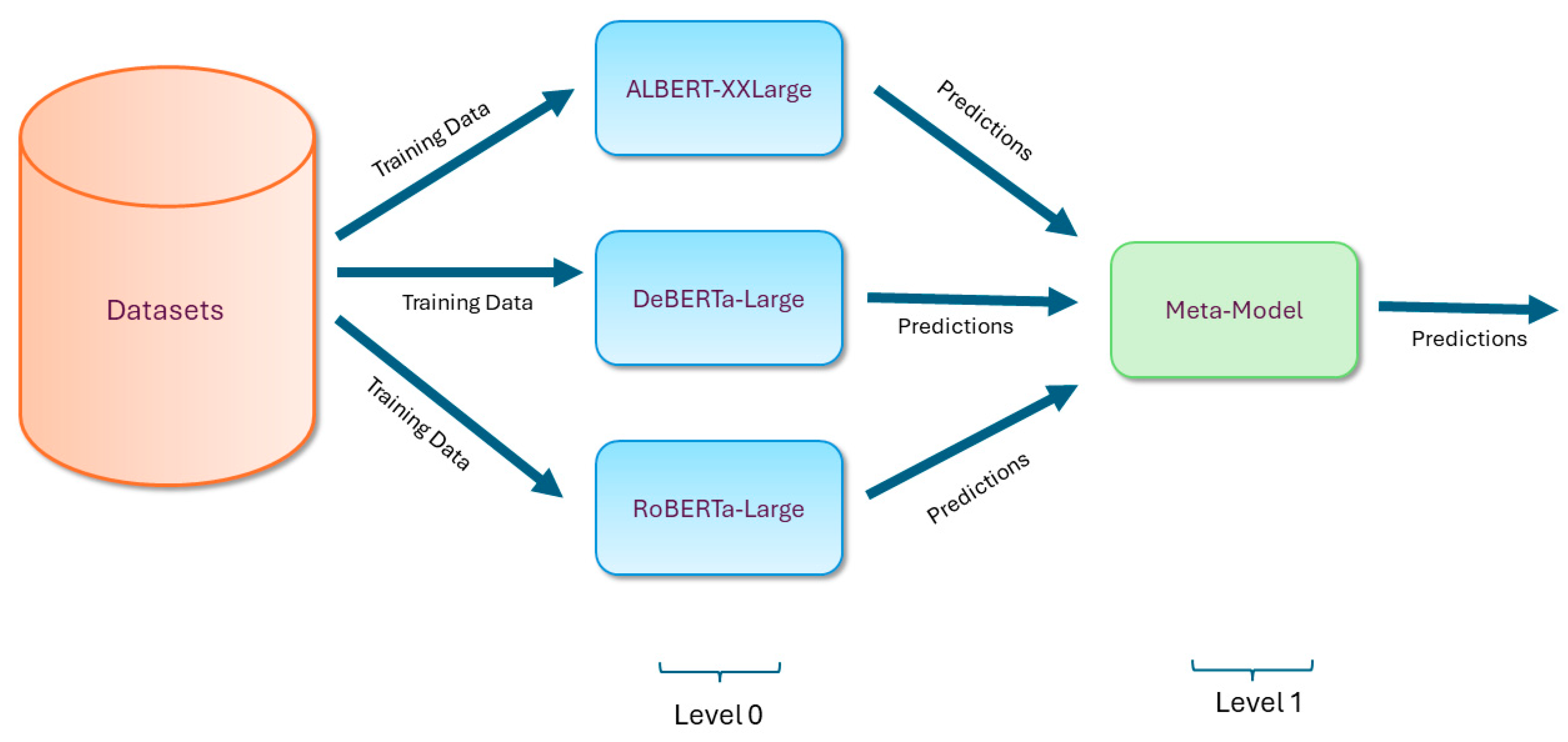
3.2. Ensemble Models Formulated

Ensembling seeks to aggregate the results of two or more models with the aim of enhancing their performance and reliability, as well as strength. They are beneficial since they try to harness the relative merits of various models in order to offer several significant advantages. Ensembling enhances accuracy by using several models to make predictions and averaging the results which lowers the variance of the particular model. This method also improves the degree of robustness and makes the model that is generated less prone to overfitting or to the biases that exist in training data [28]. In this regard, it becomes necessary to identify the right models that will be useful for ensembling purposes in NLI. Thus, the choice of these particular models can be explained by their stability and efficiency in solving NLI problems.

The first model named ynie/albert-xxlarge is based on ALBERT-XXLarge and demonstrated good results with a small number of parameters. The second model named ynie/roberta-large, based on Roberta-Large, showed a high performance because of large-scale pretraining and fine-tuning that was performed on NLI datasets. Finally, the DeBERTa-based model named deberta-large-mnli has other separate attention parts and improved embedding in comparison with other models in this list, and therefore, it can better analyze details within texts. These models integrate efficiency with high performance, showing how they balance when performing the natural language inference (NLI) tasks. All the above are fine-tuned versions of high-efficiency high-performance models.

There are various ensemble learning strategies, each with special qualities and uses. Bagging, boosting, and stacking are the main ensemble learning strategies. Training several instances of a model on various subsets of the same dataset and then aggregating their predictions using weight-voting is known as bagging or bootstrap aggregating [29]. Usually, this parallel method makes use of homogeneous models, which denote that each instance is of the same kind. A different strategy is used in the case of boosting, which involves training models one after the other sequentially with the goal of fixing the mistakes made by the previous model [30]. This methodology is predicated on a set of uniform models. Using meta-learning to combine the outputs of multiple model types that are trained, typically in parallel, is a more sophisticated ensemble technique called stacking [31]. Due to the heterogeneity of this technique, selecting different base models is possible with more flexibility. In most cases, stacking makes use of a meta-model, also known as a meta-learner, which aggregates and learns from the outputs of the base models to produce the final forecast.

Out of the different ensemble techniques, we selected stacking in our framework as it is one powerful method to incorporate benefits from a large number of finite models and enhance overall performance. Stacking provides specific benefits in natural language inference (NLI), which requires complex linguistic patterns and reasoning, that can boost performance relatively: accuracy-wise, robustness-wise, and generalization-wise [32].

Thus, we created a stacking-ensemble schema that consist of three diverse and well-performing transformer models (Figure 1). The first model of the stacking ensemble we designed is the ALBERT-XXLarge, which demonstrated good results with small number of parameters. The second model is the Roberta-Large, which has also shown a quite good performance, and the third model in the ensemble is the DeBERTa-based model, which has separate attention parts and improved embeddings in comparison with other models. The ensemble schema seeks to aggregate the results of the models with the aim of enhancing their performance and reliability. This ensemble approach also improves the degree of robustness and makes the overall schema less prone to overfitting or to the biases that exist in training data [28].

To build a robust and adaptable NLI ensemble, we chose three datasets SNLI, MNLI, as well as ANLI with all three rounds. We start from SNLI, the largest publicly available corpus from pairs of sentences with relation labels. Its examples are usually straightforward and are gathered from the images and image captions, therefore making it suitable for training large datasets for purpose of testing accuracy and validity. MNLI incorporates additional topics and sources of text, such as literature, dialogs, and government reports, and a matched and mismatched split for evaluating model robustness across these data types. It increases the versatility and stability of the ensemble in diverse conditions. ANLI introduces adversarial examples, with three increasing levels of difficulty, to encourage the model to not only understand context but also consider the variations of language forms. This syncretic approach helps guarantee that the ensemble is capable of addressing a wide range of NLI tasks.

In case of Meta-Models, we use simple and effective neural networks or frameworks, some of them being Logistic Regression, Feed-forward Neural Networks, CapsuleNet, and more. The following analysis pertains to the meta-models employed in our stacking ensemble technique, which utilized the previously mentioned base models. Note that in several cases we also introduce feature engineering in order to obtain the best results of each model. In ensemble techniques like stacking, confidence margin is used to weigh the contributions of individual models based on their confidence levels. Models with higher confidence in their predictions are given more weight in the final decision. Entropy is also used for weighing the more beneficial and appropriate models in the ensemble. Since the less uncertain model yields or holds a higher entropy than the more informative model, it is more appropriate to assign higher weights to models that offer less entropy while doing the opposite to models with higher entropy. Prediction difference quantifies how varied the predictions of the base models are. Models that are more diverse (less correlated with others) are given higher weights. With the help of multi-head attention, a powerful extension of the attention process, models can concurrently focus on multiple elements of the input data. Better performance in tasks such as language processing and graph-based learning can be achieved by the model by capturing a fuller and more nuanced knowledge of the data through the use of many attention heads, each concentrating on various relationships or sections of the input.

The “Simple” models refer to the baseline versions of the meta-models that do not incorporate any additional features. The “Featured” models in the table incorporate additional features during the ensemble learning process, like Prediction Difference and Confidence Margin, to enhance their performance. The “Featured E” variations in the meta-models refer to versions of the models that incorporate entropy as a feature during the ensemble learning process. The “Enhanced” version of the Graph Attention Network (GAT) refers to a variation that incorporates both the Confidence Margin and multi-head attention as additional features. The Bidirectional version of LSTM improves upon the standard LSTM by processing sequences in both forward and backward directions using two LSTM layers. In addition, the attention LSTM version incorporates an attention mechanism.

Regarding the experimental environment, training times varied depending on the model size and the specific task; all models were trained on one Tesla P100-PCIE-16GB using deep-learning frameworks like PyTorch 2.1.2 and TensorFlow 2.15.0. Evaluation metrics were computed on standard test sets to ensure that the reported accuracy and loss scores are both reliable and comparable across different models.

4. Experimental Study

4.1. Datasets on NLI

We used several datasets in our study and each one captures a distinct feature of NLI. So, we are able to thoroughly analyze and improve the performance of our models across a variety of linguistic and contextual issues by using a variety of datasets in our research. The datasets used are the following:

The MNLI (multi-genre natural language inference) dataset [33] is helpful for training multiclass NLI applications, containing over 400,000 sentence pairs from sources like fictional books, conversations, and government reports. MNLI challenges language models with two evaluation frameworks: Matched (MNLI-m) and Mismatched (MNLI-mm). MNLI-m focuses on discriminatory learning, while MNLI-mm tests generalization. The dataset includes sentences that clearly indicate entailment, contradiction, or neutrality, supported by diverse linguistic structures and logical relationships through crowd-sourced annotations. This diversity is valuable for advancing NLI technologies.

The adversarial natural language inference (ANLI) dataset [34] consists of sentences requiring high-accuracy inference of language subtleties, created by human annotators on complex scenarios. ANLI’s adversarial, iterative setup consists of three cycles (A1, A2, A3), targeting model vulnerabilities using diverse sources like Wikipedia, books, and articles. This approach enhances model robustness and comprehension, making ANLI a stringent benchmark for advancing NLP’s understanding of inference and implication. ANLI aims to elevate AI systems to complex natural language reasoning, setting a new standard in AI development.

The Winograd schema challenge natural language inference (WNLI) dataset [35] is crucial for NLI research, focusing on machine understanding and human language processing. Part of the GLUE benchmark, WNLI tests AI models on coreference resolution within NLI tasks, requiring interpretation of relationships between sentences through subtle linguistic cues. The dataset includes examples that demand sophisticated common-sense knowledge and reasoning, beyond simple syntactic or lexical analysis. This complexity makes WNLI invaluable for advancing NLI research by challenging AI language systems’ understanding of human language. Our study uses the WNLI dataset to address these challenges, highlighting current models’ shortcomings in complex real-world scenarios requiring nuanced understanding and reasoning.

The question-answering natural language inference (QNLI) dataset [33] is used in various NLI research. It uses the SQuAD dataset, transforming it into a binary classification task where each question–sentence pair is labeled as entailment or not entailment. QNLI’s high-quality, varied examples reflect real-world language challenges, making it ideal for evaluating NLI model performance. As part of the GLUE benchmark, QNLI aids in assessing language understanding. It also allows for investigating nuances in question-answering contexts, enhancing model comprehension capabilities.

The Stanford natural language inference (SNLI) corpus [36] consists of 570,000 human-annotated sentence pairs and aids in large-scale and diverse high-quality evaluation procedures of NLI models. It plays a key role in promoting understanding of how computational models work for comprehension of human language, what they reason about sentence relationships, and how they adapt to various linguistic contexts. SNLI is extremely important for this project because it provides good generalization for the wide scope of training data and very challenging test examples, which is exactly what is needed to push the frontier of what is possible for a model to master complex language-based tasks.

The recognizing textual entailment (RTE) dataset [33] covers various linguistic phenomena, such as synonymy, antonymy, and paraphrasing, to test models’ understanding of nuanced language. Its structured format supports systematic training and benchmarking, aiding researchers in measuring progress. The dataset’s large scale and diversity make entailment models more generalizable and robust, which is vital for real-world applications. In our NLI research, RTE is essential for developing refined models and ensuring our results meet community standards, driving collective advancements in NLI systems.

4.2. Results Analysis

In this section, we will compare the performance and losses of individual transformer models on different NLI datasets. This evaluation provides us with insight into each of the model’s advantages and disadvantages. When comparing these models with different tasks, we are able to learn how they generalize and perform with respect to the inherent challenges present in NLI.

The performance results of several transformer-based models (BERT, ALBERT, DeBERTa, RoBERTa, etc.) and their variations are shown in

Table 1. Results on every individual model and its variations across important NLI tasks. The best results are shown in bold while the second best are underlined.

	VARIATIONS	ANLI	MNLI	MNLI-m/MNLI-mm	QNLI	RTE	WNLI	SNLI
BERT	-Base	-	84.0	84.6/83.4	90.5	66.4	-	-
	+ASA	50.4	91.4	-	-	-	-	-
	+SMART	-	85.8	85.6/86.0	92.7	71.2	-	-
	+STraTA, Few-shot learning	-	-	-	82.1	70.6	-	85.7
	-Large	-	86.3	86.7/85.9	92.7	70.1	-	-
	+STraTA	-	-	-	86.4	77.1	-	87.3
ALBERT	-Base V1	-	81.6	-	-	-	-	-
	-Base V2	-	84.6	-	-	-	-	-
	-Large V1	-	83.5	-	95.2	-	-	-
	-Large V2	-	86.5	-	-	-	-	-
	-XLarge V1	-	86.4	-	95.2	88.1	-	-
	-XLarge V2	-	87.9	-	-	-	-	-
	-XXLarge V1	-	90.8	-	95.3	89.2	91.8
	-XXLarge V2	-	90.6	-	-	-	-	-
DeBERTa	-Base V1	-	88.2	-	-	-	-	-
	-Base V3	-	90.7	90.6/90.7	-	-	-	-
	-Large V1	57.6	91.2	91.3/91.1	95.3	-	-	-
	+ASA	58.2	-	-	-	-	-	-
	-Large V3	-	91.9	91.8/91.9	96.0	92.7	-	-
	XLarge V1	-	91.4	91.5/91.2	93.1	-	93.2	-
	XLarge V2	-	91.7	91.7/91.6	95.8	93.9	-	-
	XXLarge	-	91.8	91.7/91.9	96.0	93.5	-	-
	+LoRA	-	91.9	-	96.0	94.9	-	-
RoBERTa	-Base	33.2	87.6	-	92.8	78.7	-	-
	+LoRA	-	87.5	-	93.3	86.6	-	-
	+MUPPET	-	88.1	-	93.3	87.8	-	-
	+InfoBERT (FreeLB)	34.4	-	-	-	-	-	-
	+InfoBERT (ST) (MNLI + SNLI)	-	90.5	90.5/90.4	-	-	-	93.3
	+InfoBERT (AT) (MNLI + SNLI)	-	90.6	90.7/90.4	-	-	-	93.1
	+(ST) (MNLI + SNLI)	-	90.7	90.8/90.6	-	-	-	92.6
	+(AT) FreeLB (MNLI + SNLI)	-	90.2	90.1/90.3	-	-	-	93.4
	+ASA	-	88.0	-	93.4	-	-	-
	-Large	51.9	90.2	-	94.7	89.5	-	-
	+MNLI	-	90.2	-
	+LoRA	-	90.6	-	94.9	87.4	-	-
	+LoRA (finetuned)	-	90.2 *	-	94.7	86.6	-	-
	+SMART	57.1	91.2	91.1/91.3	95.6	92.0	-	-
	+SMART (MNLI + SNLI + ANLI_FEVER)	57.1		-	-	-	-	-
	+EFL	-		-	94.5	90.5	-	93.1
	+ALUM	57.7	90.6	90.9/90.2	95.1	-	-	93.0
	+ALUM and SMART	-	-	-	-	-	-	93.4
	+I-BERT	-	90.4	90.4/90.3	94.5	87.0	-	-
ERNIE	-1.0	-	83.6	84.0/83.2	91.3	68.8	-	-
	-2.0 (Base)	-	85.8	86.1/85.5	92.9	74.8	65.1	-
	-2.0 (Large)	-	88.3	87.7/88.8	94.6	85.2	67.8	-
T5	-Base	86.7	86.7	87.1/86.2	93.7	80.1	78.2	-
	-Large	89.8	89.8	89.9/89.6	94.8	87.2	85.6	-
	+explanation prompting (LP)	52.8	-	-	-	-	-	-
	+explanation prompting (EP)	71.0	-	-	-	-	-	-
	-3 B	-	91.3	91.4/91.2	96.3	91.1	89.7	-
	+explanation prompting (EP)	76.4	-	-	-	-	-	-
	-11 B	-	92.2	92.2/91.9	96.9	92.8	94.5	-
ELECTRA	-400 K	-	90.5	-	94.5	85.9	-	-
	-1.75 M	-	90.9	-	95.0	88.0	-	-
XLNet	-Large	-	88.4	-	93.9	81.2	-	-
Vega v2	-Base	-		-		96.0	-	-

for a number of natural language inference (NLI) tasks, such as ANLI, MNLI, QNLI, RTE, WNLI, and SNLI. The values in the columns under each NLI task indicates the accuracy expressed as a percentage achieved by that model on that particular task. Each row represents a different model or variant. Specifically in classification tasks, accuracy is a performance statistic that is used to assess a model’s efficacy. Accuracy, as used in NLI tasks, is the percentage of the model’s total number of predictions that are accurate. With an accuracy of 84% (as shown in Table 1), the model identified the label (such as entailment, contradiction, or neutral) correctly for 84 out of 100 cases that were examined. Accuracy is a straightforward method to measure the model’s frequency of providing the right response and is most useful when the classes in the dataset are balanced. Formula for accuracy:

$$Accuracy={\displaystyle \frac{NumberofCorrectPredictions}{TotalNumberOfPredictions}}$$

As for the experimental environment, training times varied depending on the model size and the specific task. Additionally, evaluation metrics were computed on standard test sets, ensuring that the reported accuracy scores are both reliable and comparable across different models.

As shown in Table 1, BERT demonstrates strong performance across various NLP tasks. Techniques like adversarial self-ensembling (ASA) and SMART enhance BERT-Base’s performance without adding complexity, while few-shot learning with STraTA maintains overall efficiency despite minor declines.

ALBERT models show various benefits, especially from V1 to V2 versions. ALBERT-Base V2 improves MNLI performance by 3.7% over V1 with the same layers and parameters. ALBERT-XLarge V2 performs 26% better in RTE than BERT-Large. ALBERT-XXLarge V1 surpasses BERT-Large in QNLI and RTE by 2.8% and 27.3%, respectively, with 223 M parameters and 12 layers. However, using adapters negatively impacts performance. ALBERT-XXLarge with adapters performs 4.5% worse in QNLI and 25.5% worse in WNLI. Despite having fewer parameters (12 M), ALBERT-Base V2 achieves results comparable to BERT-Base, particularly in MNLI.

The DeBERTa model family shows improved performance with increased complexity and architectural refinements. DeBERTa-Base V3 outperforms V1 in MNLI by 2.8% with the same parameters (100 M) and layers (12). DeBERTa-Large V3 improves by 1.7% in MNLI and shows gains in QNLI and RTE with the same parameters (350 M) and layers (24). DeBERTa-XLarge V2 slightly improves over V1 in MNLI and excels in RTE and QNLI, further optimized with techniques like LoRA. DeBERTa models consistently outperform their predecessors and competitors. DeBERTa-Base V3 surpasses BERT-Base and ALBERT-Base V2 in MNLI, despite having fewer parameters than BERT-Base. DeBERTa-Large V3 outshines BERT-Large and ALBERT-Large V2 in MNLI and QNLI. DeBERTa-XLarge V2 exceeds BERT-Large in MNLI and RTE, demonstrating advanced capabilities. While DeBERTa models generally have higher complexity, their performance gains justify the increased parameters and layers. The ALBERT models deliver strong results with fewer parameters and layers.

The RoBERTa model family includes several variations with significant differences in layers and parameters, impacting their NLI task performance. RoBERTa-Base has 12 layers and 125 million parameters, while RoBERTa-Large, with 24 layers and 355 million parameters, shows gains of 3% in MNLI, 2% in QNLI, and 14% in RTE. Advanced techniques like LoRA and SMART further improve performance in tasks like ANLI and RTE. RoBERTa-Base outperforms BERT-Base in MNLI, QNLI, and RTE, showing superior optimization. Compared to ALBERT and DeBERTa, RoBERTa variants generally perform better despite having more parameters and layers.

ERNIE-2.0 Base, with 103 million parameters and the same number of layers, surpasses its predecessor by around 3% in MNLI and QNLI and by 9% in RTE. ERNIE-2.0 Large, with three times the parameters and double the layers of ERNIE-1.0, achieves performance gains of 5.6% in MNLI, 3.7% in QNLI, and 24% in RTE. Comparing ERNIE-2.0 Base to DeBERTa-Base and RoBERTa-Base, ERNIE performs slightly worse by 2.7% and 2% in MNLI, respectively, and similarly in QNLI, but falls short by 5% in RTE. ERNIE-2.0 Large performs 2% better in MNLI than DeBERTa-Large V3 but 4% worse in QNLI and 8% worse in RTE. Despite similar sizes, ERNIE models generally lag behind DeBERTa and RoBERTa in most benchmarks, highlighting that performance differences are due to model architecture and training techniques rather than size alone.

The T5 model family demonstrates improved performance with increasing size and complexity. T5-Base expands to 24 layers and 220 million parameters. T5-Large retains 24 layers but grows to 770 million parameters. T5-3B further increases to 48 layers and 3 billion parameters, and T5-11B reaches 48 layers and 11 billion parameters. Performance improves with size: T5-11B achieves 92.2% accuracy on MNLI, outperforming T5-3B by 2.7% and T5-Large by 1%. T5-Base scores 86.7%. For QNLI, T5-11B leads with 96.9%, followed by T5-3B at 96.3%, and T5-Large at 94.8%. T5-Base performed lower. On WNLI, T5-11B scores 94.5%, surpassing T5-3B by 5%, T5-Large by 9.4%, and T5-Base by 17.3%. T5-Large also excels in ANLI, improving by 3.6% over T5-Base. Overall, T5-11B sets state-of-the-art results across several tasks, showcasing the benefits of larger model sizes for performance and accuracy in NLI tasks.

The performance of ELECTRA-400K and ELECTRA-1.75M is compared to similar models like BERT-Base, BERT-Large, RoBERTa-Base, RoBERTa-Large, and DeBERTa-Base and Large. ELECTRA-400K, with 12 layers and 100–110 M parameters, outperforms BERT-Base in MNLI, QNLI, and RTE by 7.74%, 4.42%, and 29.37%, respectively, and also exceeds DeBERTa-Base by 2.61% in MNLI. ELECTRA-1.75M shows gains over BERT-Large with 5.33% in MNLI, 2.48% in QNLI, and 25.54% in RTE. It performs slightly below DeBERTa-Large in MNLI and QNLI but surpasses RoBERTa-Large in both tasks and is nearly on par in RTE. These results highlight ELECTRA’s effectiveness and reliability for high-performance NLI tasks.

When compared to other similarly sized models, XLNet-Large performs competitively. It surpasses BERT-Large in MNLI, QNLI, and RTE by 2.43%, 1.29%, and 15.85%, respectively. However, it slightly lags behind DeBERTa-Large and RoBERTa-Large in MNLI and QNLI by 0.85% and 2.19% and 2.00% and 3.07%, respectively. In RTE, XLNet-Large outperforms BERT-Large but trails RoBERTa-Large by 9.27%. Overall, XLNet-Large demonstrates strengths in NLI tasks but is outperformed by some competitors in specific cases. Models like DeBERTa-XXLarge + LoRA, DeBERTa-XLarge V2, and ALBERT-XXLarge V1 offer competitive results with fewer parameters and layers. Vega V2 achieves the highest performance on the RTE benchmark at 96.0%.

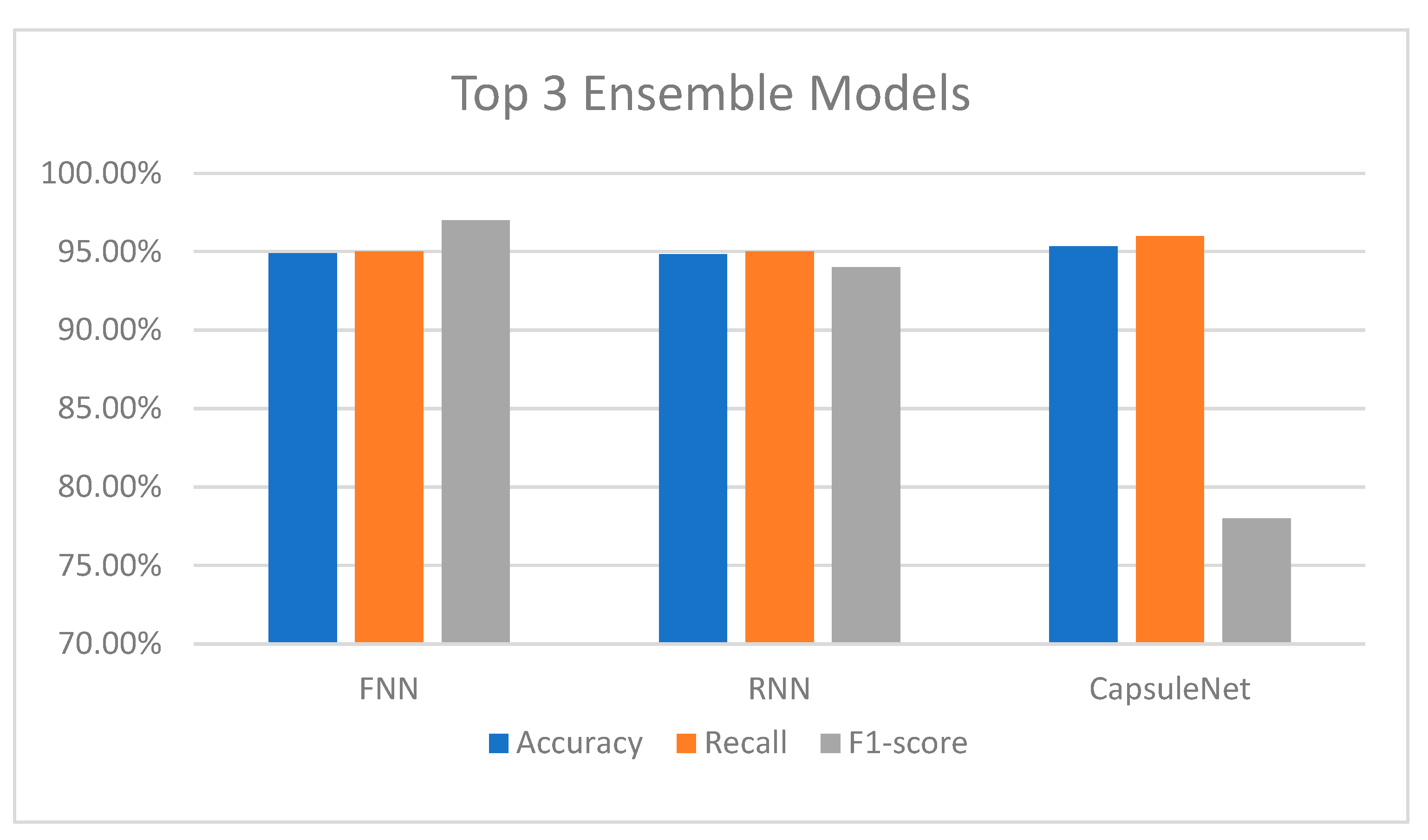
4.3. Results of the Ensemble Models

In this section, we present the outcomes of our experiments on the stacking-ensemble models focusing on the effectiveness and their performance of various techniques in natural language inference (NLI) tasks. We evaluate the results using different model architectures and methods to determine their impact on accuracy and robustness. Our primary objective is to identify the best approaches for improving the performance of the NLI approaches.

In

Table 2. Accuracy and loss on every meta-model and its variations across important NLI tasks. The best results are shown in bold.

Meta Model	Variation	SNLI ACC/LOSS	MNLI-m ACC/LOSS	MNLI-mm ACC/LOSS	ANLI R1 ACC/LOSS	ANLI R2 ACC/LOSS	ANLI R3 ACC/LOSS
Logistic Regression	-Simple	93.13%/0.21	92.00%/0.22	91.61%/0.25	70.50%/0.70	73.50%/0.72	69.58%/0.67
	-Featured	93.18%/0.21	92.40%/0.22	91.66%/0.25	72.00%/0.71	73.50%/0.73	68.75%/0.68
	-Featured E	93.12%/0.21	92.05%/0.22	91.76%/0.25	71.00%/0.71	73.50%/0.74	68.75%/0.69
GBM (XGBoost)	-Simple	92.84%/0.47	92.01%/0.48	91.82%/0.31	78.00%/0.61	67.25%/0.78	69.58%/0.79
	-Featured	92.88%/0.54	92.30%/0.45	91.51%/0.51	67.50%/0.87	68.50%/0.87	73.33%/0.83
	-Featured E	93.02%/0.59	91.90%/0.58	91.56%/0.60	68.00%/0.83	69.50%/0.90	75.00%/0.76
FNN	-Simple	93.68%/0.20	92.26%/0.20	91.71%/0.22	74.00%/0.70	66.00%/0.81	61.67%/0.79
	-Featured	96.36%/0.12	96.93%/0.13	96.44%/0.15	74.41%/0.51	77.78%/0.66	67.92%/0.66
SVC	-Simple	93.49%/0.07	90.84%/0.10	91.77%/0.08	77.00%/0.23	64.00%/0.36	49.17%/0.51
	-Featured	95.53%/0.10	96.25%/0.09	96.62%/0.08	74.42%/0.65	68.89%/0.74	45.28%/1.33
RNN	-Simple	93.23%/0.22	91.90%/0.22	91.76%/0.26	71.50%/0.78	74.00%/0.74	70.41%/0.68
	-Featured	96.52%/0.12	97.10%/0.12	96.28%/0.15	74.42%/0.54	77.78%/0.66	66.03%/0.67
GCN	-Simple	93.13%/0.21	92.10%/0.23	91.87%/0.25	71.50%/0.71	74.50%/0.73	70.42%/0.67
	-Featured	95.69%/0.17	96.33%/0.15	96.70%/0.12	82.56%/0.40	73.03%/0.65	71.70%/0.64
GAT	-Featured	95.44%/0.17	96.16%/0.15	96.62%/0.13	83.72%/0.39	73.03%/0.65	63.70%/0.64
	-Enhanced	95.44%/0.17	96.59%/0.16	96.62%/0.13	83.72/0.45	75.28%/0.70	72.64%/0.67
LSTM	-Simple	93.20%/0.22	92.00%/0.23	91.80%/0.25	71.50%/0.76	74.50%/0.75	69.20%/0.67
	-Featured	96.19%/0.12	96.93%/0.12	96.28%/0.15	74.42%/0.52	77.78%/0.68	66.04%/0.68
	-Bidirectional	96.35%/0.12	97.10%/0.12	96.45%/0.15	74.42%/0.51	77.78%/0.66	67.90%/0.67
	-Attention	96.36%/0/12	96.93%/0.12	96.45%/0.15	74.42%/0.50	73.33%/0.67	66.03%/0.68
CapsuleNet	-Simple	93.44%/0.21	92.21%/0.22	92.12%/0.24	72.50%/0.75	74.50%/0.76	71.25%/0.72
	-Featured	95.69%/0.17	96.67%/0.14	96.79%/0.12	81.40%/0.52	71.91%/0.82	74.53%/0.75

, we present the outcomes of multiple meta-models and their differences in key natural language inference (NLI) tasks, such as ANLI rounds 1, 2, and 3; MNLI-m; MNLI-mm; and SNLI. With an astounding 96.52% accuracy, the RNN (Featured) model achieves the top results for the SNLI challenge. This model performs 0.17% better than LSTM (Bidirectional), the next best model, demonstrating its improved handling of the SNLI dataset. Multiple models, such as the RNN (Featured), LSTM (Bidirectional), and LSTM (Attention) models, obtain the lowest cumulative loss of 0.12 in terms of loss, implying that these models are very effective and well-generalized for this particular job. The above analysis demonstrates the effectiveness of RNN (Featured) in the SNLI task.

The RNN (Featured) model outperforms the LSTM (Bidirectional) model by 0.16% on the MNLI-m task, achieving the greatest accuracy of 97.10%. This small but notable difference illustrates how well the RNN (Featured) model performs on this dataset. RNN (Featured), LSTM (Bidirectional), and LSTM (Attention) all have the lowest loss for this task, which is 0.12, indicating that these models are equally good at reducing errors. Consequently, RNN (Featured) once again reports the best performance on MNLI-m.

With an accuracy of 96.79% for the MNLI-mm task, CapsuleNet (Featured) outperforms the second-best model (LSTM Bidirectional) by 0.14%. This tiny advantage reflects CapsuleNet’s enhanced performance with this dataset. CapsuleNet (Featured) and GAT (Enhanced) have the lowest combined loss, both at 0.12. To sum up, CapsuleNet (Featured) tends to perform at the top of the MNLI-mm task.

With 83.72% accuracy, GAT (Featured) and GAT (Enhanced) share the best accuracy for the ANLI R1 challenge. This shows that these models have an exceptional level of ability to manage the dataset’s complexity. GAT (Enhanced) has a loss of 0.45, whilst GAT (Featured) has the lowest loss of 0.39, 10.87% better. This huge loss reduction demonstrates how effective GAT (Featured) is at reducing errors.

With respective scores of 77.78%, the LSTM (Bidirectional) and RNN (Featured) models obtain the finest accuracy for the ANLI R2 task. Although with the lowest loss of 0.65, GAT (Featured) outperforms the next best model, LSTM (Bidirectional), by 1.54%, LSTM (Bidirectional) is the optimal model for this particular task.

CapsuleNet (Featured) has the highest accuracy of 74.53% for the ANLI R3 task, exceeding GCN (Simple), the next best model, by 2.59%. This significant improvement highlights the superior performance of CapsuleNet on this dataset. GCN (Featured) achieves the lowest combined loss for this task at 0.64, which is 1.54% better than the LSTM (Bidirectional) model at 0.67. This shows how effective GCN (Featured) is at reducing errors for this assignment. The top model is CapsuleNet (Featured), which performs exceptionally well on a variety of tasks; with MNLI-mm (96.79%) and ANLI R3 (74.53%), it attains the highest accuracy, showcasing its exceptional performance regarding these datasets. In other tasks, like SNLI (95.69%) and MNLI-m (96.67%), CapsuleNet (Featured) also maintains competitive accuracy. Additionally, CapsuleNet (Featured) has low combined loss values in the MNLI-m, MNLI-mm, and SNLI tasks, where its best loss is 0.12. This suggests that CapsuleNet (Featured) is efficient, well-generalized, and accurate. Based on the results of each of the models that were assessed, it is the most resilient and reliable meta model choice because of its continuous high performance and low loss in a variety of NLI tasks.

The recall and F1-score metrics on the same NLI tasks of the models are presented in

Table 3. Recall and F1 score on every meta-model and its variations across important NLI tasks.

Meta Model	Variation	SNLI Recall/F1-Score	MNLI-m Recall/F1-Score	MNLI-mm Recall/F1-Score	ANLI R1 Recall/F1-Score	ANLI R2 Recall/F1-Score	ANLI R3 Recall/F1-Score	Combined Tasks Recall/F1-Score
Logistic Regression	-Simple	0.93/0.93	0.92/0.92	0.92/0.92	0.71/0.71	0.74/0.74	0.70/0.70	0.89/0.89
	-Featured	0.93/0.93	0.92/0.92	0.92/0.92	0.72/0.72	0.73/0.74	0.69/0.68	0.90/0.90
	-Featured E	0.93/0.93	0.92/0.92	0.92/0.92	0.71/0.71	0.73/0.74	0.68/0.68	0.90/0.90
GBM (XGBoost)	-Simple	0.93/0.93	0.92/0.92	0.92/0.92	0.69/0.69	0.70/0.70	0.70/0.70	0.89/0.89
	-Featured	0.93/0.93	0.92/0.92	0.92/0.92	0.68/0.67	0.69/0.69	0.73/0.73	0.90/0.90
	-Featured E	0.93/0.93	0.92/0.92	0.92/0.92	0.68/0.68	0.69/0.70	0.75/0.75	0.92/0.92
FNN	-Simple	0.95/0.93	0.93/0.92	0.92/0.91	0.75/0.71	0.66/0.61	0.64/0.54	0.90/0.89
	-Featured	0.96/0.98	0.97/0.98	0.96/0.98	0.72/0.82	0.71/0.92	066/0.88	0.95/0.97
SVC	-Simple	0.94/0.93	0.91/0.91	0.92/0.92	0.77/0.77	0.64/0.65	0.50/0.48	0.89/0.90
	-Featured	0.72/0.75	0.66/0.65	0.67/0.66	0.66/0.61	0.62/0.61	0.33/0.21	0.70/0.72
RNN	-Simple	0.93/0.92	0.92/0.92	0.92/0.91	0.70/0.68	0.69/0.69	0.69/0.68	0.89/0.89
	-Featured	0.97/0.96	0.97/0.96	0.96/0.95	0.74/0.72	0.78/0.77	0.68/0.64	0.95/0.94
GCN	-Simple	0.93/0.93	0.92/0.92	0.92/0.92	0.72/0.72	0.75/0.75	0.70/0.70	0.90/0.90
	-Featured	0.77/0.80	0.69/0.70	0.68/0.69	0.79/0.79	0.73/0.74	0.72/0.70	0.74/0.76
GAT	-Featured	0.95/0.95	0.96/0.95	0.97/0.95	0.80/0.80	0.75/0.75	0.74/0.72	0.95/0.94
	-Enhanced	0.95/0.05	0.97/0.96	0.96/0.95	0.84/0.84	0.75/0.75	0.73/0.70	0.95/0.94
LSTM	-Simple	0.93/0.93	0.92/0.92	0.92/0.92	0.72/0.72	0.74/0.75	0.69/0.69	0.89/0.89
	-Featured	0.79/0.81	0.70/0.72	0.70/0.71	0.69/0.68	0.74/0.74	0.66/0.61	0.74/0.76
	-Bidirectional	0.78/0.81	0.72/0.75	0.70/0.71	0.69/0.68	0.76/0.76	0.64/0.60	0.73/0.76
	-Attention	0.78/0.80	0.72/0.75	0.70/0.71	0.69/0.68	0.76/0.76	0.65/0.60	0.74/0.76
CapsuleNet	-Simple	0.93/0.93	0.91/0.91	0.92/0.92	0.70/0.70	0.74/0.74	0.70/0.70	0.89/0.89
	-Featured	0.96/0.81	0.96/0.71	0.97/0.69	0.86/0.80	0.76/0.73	0.78/0.72	0.96/0.78

. Remarkably, models like CapsuleNet and RNN, which demonstrated excellent performance in Table 2, still maintain good recall and F1-score. Specifically, the RNN (Featured) model, which ranked highly in terms of accuracy and loss achieves particularly high recall and F1-scores across various NLI tasks, with near-perfect scores on MNLI-m (0.97/0.96) and MNLI-mm (0.96/0.95). Additionally, CapsuleNet models consistently perform well in both combined and ANLI R3 tasks, maintaining a high recall across a variety of tasks with a standout performance in the ANLI R3 and combined tasks. However, the CapsuleNet (Featured) model has a considerable decline in F1-scores, suggesting that although it exhibits the highest accuracy marked, the model might not be as good at preserving a balance between recall and precision. Another interesting finding is that certain models, such as SVC (Featured), despite having good accuracy metrics, exhibit a notable decrease in recall and F1-score, especially when it comes to the ANLI tasks. This implies that while these models may work rather seamlessly in their general operations, they may face issues with specific features of datasets, perhaps in sampling, or in categorization of all the relevant samples. Another example of such discrepancies is the LSTM (Bidirectional) model that had lower Recall and F1-score, particularly in the ANLI tasks, but demonstrated good results in both Table 2, accuracy and loss. Altogether, accuracy and loss give a fundamental comprehension of the performance of the models, while recall and F1-score provide a vital viewpoint on the capability of the model to decrease errors and accurately predict the classes.

Table 4. Meta models used in the ensembling technique evaluated on accuracy and loss over SNLI + MNLI-m + MNLI-mm + ANLI rounds 1, 2, 3. The best results are shown in bold.

Meta Model	Variation	Accuracy Combined	Loss Combined	Cross Validation Accuracy	Cross Validation Loss	Folds	Features
Logistic Regression	-Simple	89.32%	0.31	89.72%	0.31	5	-
	-Featured	90.05%	0.29	90.07%	0.28	5	Prediction Difference
	-Featured E	89.97%	0.29	90.00%	0.29	5	Entropy
GBM (XGBoost)	-Simple	-	-	90.02%	0.27	5	-
	-Featured	89.95%	0.54	89.00%	0.60	5	Prediction Difference
	-Featured E	90.05%	0.63	89.96%	0.67	5	Entropy
FNN	-Simple	89.67%	0.28	-	-	-	-
	-Featured	94.89%	0.16	-	-	-	Confidence Margin
SVC	-Simple	89.47%	0.11	-	-	-	-
	-Featured	94.32%	0.13	-	-	-	Confidence Margin
RNN	-Simple	89.16%	0.31	-	-	-	-
	-Featured	94.84%	0.17	94.75%	0.18	5	Confidence Margin
GCN	-Simple	90.10%	0.29	89.51%	0.30	5	-
	-Featured	94.61%	0.19	94.53%	0.18	5	Confidence Margin
GAT	-Featured	94.51%	0.19	94.61%	0.18	5	Confidence Margin
	-Enhanced	94.40%	0.19	94.88%	0.18	5	Confidence Margin + multi-head attention
LSTM	-Simple	89.32%	0.30	-	-	-	-
	-Featured	94.84%	0.17	94.75%	0.18	5	Confidence Margin
	-Bidirectional	94.84%	0.17	94.75%	0.17	5	Confidence Margin
	-Attention	94.74%	0.17	94.74%	0.17	5	Confidence Margin
CapsuleNet	-Simple	89.44%	0.30	-	-	-	-
	-Featured	95.33%	0.16	-	-	-	Confidence Margin

provides the analysis that follows, which compares the accuracy and loss of the meta models employed in the ensembling technique regarding the combination of SNLI + MNLI-m + MNLI-mm + ANLI rounds 1, 2, and 3. It is clear from evaluating the effectiveness of several Logistic Regression model variants that adding more variables and entropy measurements results in appreciable gains in accuracy and loss metrics. The Simple Logistic Regression model yielded an accuracy of 89.32%. The accuracy rose to 90.05%, or a percentage gain of about 0.82%, when prediction differences were introduced in the Featured variation. Compared to the Simple variation, the Featured E variation performed 0.73% better and included entropy features. The increased entropy features did not, however, considerably improve performance over the previously enhanced Featured variation, as evidenced by the tiny drop in accuracy of approximately 0.09% when comparing the Featured and Featured E variations directly. When the combined loss was examined, the Simple variation showed a 0.31 loss. This was decreased to 0.29 by the Featured and Featured E variations, which led to a 6.5% reduction in loss. The Simple Logistic Regression model’s cross-validation accuracy was 89.72%. With the Featured version, this increased to 90.07%, a gain of almost 0.39%. Additionally, the Featured E variation outperformed the Simple variation by 0.31%. A small drop of roughly 0.08% is seen when the Featured and Featured E versions are compared. There was a 9.68% reduction in the Simple variation’s loss of 0.31, which dropped to 0.28 in the Featured version. The loss increased by 3.6% between the Featured and Featured E variations; however, the Featured E variation shows a 6.6% drop in comparison to the Simple variation. Indicating that while both feature sets improve performance over the Simple model, the prediction difference features are slightly more effective in reducing loss compared to entropy features.

Following the XGBoost model, we observe that the Simple model has a cross-validation accuracy of 90.02%. In the Featured variation, this drops to 89.00%, representing a 1.1% drop. Compared to the Simple model, the Featured E variation decreased by 0.07%. The accuracy rises by 1% when comparing the Featured and Featured E versions, indicating that entropy features better enhance the cross-validation accuracy in comparison to the prediction difference feature. The Simple variation displays a cross-validation loss of 0.27. This rises by 122% to 0.60 in the Featured variant, a significant increase. The increase from the Simple model is much higher in the Featured E version, at 148%. There is an 11.7% increase in loss when comparing the Featured and Featured E versions, demonstrating how the entropy feature further increases the model’s loss. This indicates a trade-off between slight accuracy gains and considerable loss increases when employing feature engineering with prediction differences and entropy features. When we examine all of the variations of XGBoost and Logistic Regression side by side, we find some significant distinctions. XGBoost outperforms Logistic Regression in Simple variations, showing a marginal gain in accuracy (0.8%) but a notable reduction in cross-validation loss (12.9%). Nevertheless, in the Featured versions, XGBoost shows a significant increase in loss values, whereas Logistic Regression performs better overall in terms of accuracy and cross-validation accuracy, declining by roughly 0.1% and 1.2%, respectively. In this regard, as compared to its Logistic Regression equivalent, the XGBoost model that is Featured exhibits an 86.21% increase in loss. This pattern is maintained in the Featured E versions, where XGBoost’s loss values sharply rise by 117% and 131% for combined and cross-validation loss, respectively, while its accuracy only slightly improves by 0.09%. Based on these results, we can conclude that while XGBoost delivers higher accuracy under specific circumstances, using this method translates into considerably larger loss values and, therefore, may point out the problems of overfitting or ineffectiveness if specific features are defined.

The analysis of FNN shows that the Featured variation significantly improves performance over the Simple one. There is an approximate 5.8% gain in accuracy and a 42.9% decrease in loss. These findings suggest that introducing the confidence margin as a feature significantly improves the performance of the ensemble model.

There are important distinctions between the Support Vector Classifier (SVC)’s basic and Featured versions. The accuracy provided by the Featured SVC model shows an important increase, rising by 5.41% from 89.47% to 94.32%. Nevertheless, this accuracy gain is accompanied by a greater loss, growing by 18.18%. This suggests that despite the Featured SVC model achieving higher accuracy, the minor increase in loss is the cost that it pays for its improved performance. When comparing the basic versions of SVC and Logistic Regression, SVC exhibits a significant loss decrease of 64.52% combined with a marginal gain in accuracy of 0.17%. This suggests that in its basic form, SVC performs better in terms of both accuracy and loss. With a 4.75% gain in accuracy over Logistic Regression, SVC shows a more noticeable increase when looking at the Featured variations. Furthermore, when comparing the Featured SVC model to the Featured Logistic Regression model, the loss for the former falls by 55.17%. The results obtained imply that SVC generally performs better than Logistic Regression.

Significant improvements occur with the Featured variation of the Recurrent Neural Network (RNN) when compared to the Simple variation. The Featured RNN model’s accuracy rises from 89.16% to 94.84%, a 6.37% enhancement. Likewise, the loss of the Featured RNN model drops from 0.31 to 0.17, a 45.16% decrease. This suggests that in comparison to the basic RNN model, the Featured RNN model performs much better in terms of accuracy and loss. When FNN and RNN variations are compared, it can be shown that FNN performs somewhat better than RNN in terms of combined accuracy for the Simple models, whereas RNN’s performance decreases by 0.57%. The Simple FNN model operates better overall, with a total loss which is 10.71% lower in comparison to the Simple RNN model. In terms of Featured variations, both models function similarly, with RNN exhibiting a small drop of 0.05% in comparison to FNN. Furthermore, RNN’s loss rises by 6.25%, while FNN’s combined loss stays marginally lower. These findings imply that although the accuracy of both models is equivalent, FNN consistently performs marginally better in terms of reduced loss.

There are notable improvements when comparing the GCN ensemble model with Simple and Featured variations. The combined loss falls by 34.48% while the combined accuracy rises by 5.00% from the Simple to the Featured version. In a comparable manner, the Featured GCN model’s cross-validation accuracy increases by 5.61% while the cross-validation loss drops by 40.00%. The results presented show that once compared to the basic GCN model, the Featured GCN model performs noticeably better in terms of accuracy and loss.

The comparison between the Featured and Enhanced variations of the GAT model shows minor differences. The combined accuracy for the Enhanced GAT model slightly decreases by 0.12%. However, the cross-validation accuracy improves by 0.29% from the Featured to Enhanced version. Both the combined loss and cross-validation loss remain unchanged at 0.19 and 0.18, respectively. The results obtained demonstrate that although there is a slight rise in cross-validation accuracy with the Enhanced GAT model, overall, there is no discernible difference in accuracy or loss. By comparing the Featured version of GCN with the Enhanced and Featured versions of GAT, it can be proven that GCN has a marginally lower combined accuracy (94.61%) than GAT (94.51%), with a marginal reduction of 0.11% for GAT. However, GAT reported a 0.08% boost in cross-validation accuracy. A comparable performance in terms of loss metrics is demonstrated by the equal combined loss (0.19) and cross-validation loss (0.18) for both models. The accuracy of GCN Featured remains greater than that of GAT Enhanced, which shows a 0.22% decline. Nonetheless, there is a 0.37% improvement in cross-validation accuracy with the Enhanced GAT model. In both cases, the loss values do not change. These comparisons indicate that GAT performs slightly better in cross-validation accuracy, whereas GCN has a little higher combined accuracy.

Notable variations and similarities amongst the models are shown by comparing the LSTM versions. The Featured variation of the LSTM model exhibits an impressive rise in combined accuracy of 6.18% and a major decrease in combined loss of 43.33% when compared to the Simple model. It therefore indicates that the Featured LSTM model surpasses the basic one in terms of effectiveness. Neither combined accuracy nor combined loss differ between the Bidirectional LSTM and the Featured LSTM. Last but not least, an examination between the attention LSTM and the highlighted LSTM reveals a minor drop in combined accuracy of 0.11% but no change in combined loss. This shows that, as opposed to the regular Featured LSTM, the attention mechanism somewhat lowers the model’s accuracy but has no discernible effect on loss.

Considerable progress has been made in the Featured model of CapsuleNet as compared to the Simple version. In combination, the accuracy rises by 6.58% while the loss falls by 46.67%. CapsuleNet (Featured) has the highest combined accuracy at 95.33% and one of the lowest combined loss values at 0.16.

In Figure 2 we observe that with accuracy and recall all slightly above 94% and the F1-score being the highest at over 95%, the FNN model consistently performs well across all three criteria. With all metrics circling the mid-90% area, the RNN model exhibits a similar tendency and performs quite similarly to the FNN. CapsuleNet exhibits a substantially lower F1-score which falls below 80% despite demonstrating strong performance in terms of Accuracy and Recall, both of which are above 95% and the best among the top models. This suggests that CapsuleNet fails to balance precision and recall, which results in a somewhat lower F1-score, even if it is effective in precisely identifying instances. All things considered, FNN and RNN seem to be the most balanced models in terms of performance, while CapsuleNet, even with its state-of-the-art accuracy, may need some future work.

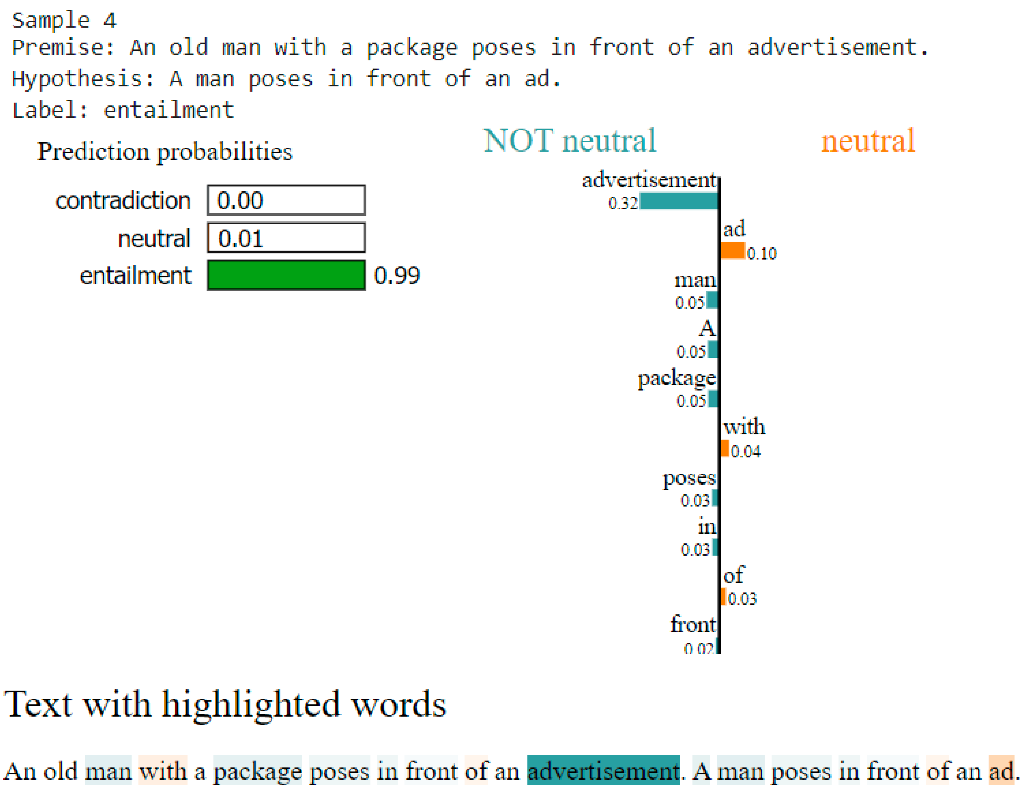
5. Models Explainability

After the performance analysis of the transformers, we apply explainability techniques to examine how our finetuned DeBERTa-Large-mnli, which was one of the best performing models, makes decisions and how it takes into account the words of the sentences and the contextual information [37]. LIME and SHAP methods are utilized to help to understand how the transformer models utilize words and contextual information in sentences in order to make their inferences [38].

LIME [39] (Local Interpretable Model-agnostic Explanations) provides insights into the predictions of complex models by using simpler, interpretable models such as linear regression or decision trees for specific instances. By modifying the input and observing the resulting changes in output, LIME identifies the key features influencing the prediction. This approach is particularly valuable for understanding which words or phrases in a text drive the model’s sentiment classification, offering clear insights into the decision-making process of the model.

SHAPs [40] (Shapley additive explanations) explain model outputs by attributing the prediction to the input features based on their contributions. It effectively highlights which words or elements of a sentence are affecting the sentiment prediction, providing a deeper understanding of the transformer’s behavior and the reasoning behind its predictions. This technique enhances the transparency and accountability of the transformer model by clearly demonstrating the contribution of each feature to the final prediction.

When working with LIME, we obtain the information about the interaction of individual cases and the decision made by the model, which is critical for debugging and optimizing its performance. SHAP further augments this by giving a more holistic view of how the model operates on different inputs and whether it has biases or systematic errors. Combined, these approaches enable the cross-verification of the hypotheses derived out of the model, and are instrumental in establishing generalizability of conclusions, besides individual case accuracy. Additionally, the employment of SHAP summary plots remains crucial for our analysis, as it facilitates the detection of global trends inherent in feature importance and thereby global structure of the model’s decision-making. The advantage of this local and global framework is that both interpretations guarantee a broad and detailed understanding of the model in order to tackle local and general issues in NLI.

We illustrate for various example cases, the premises, the hypothesis, the label in terms of contradiction, neutrality (neutral), or entailment and the way that LIME and SHAP assist in interpreting the transformer model’s prediction.

In Figure 3, the premise is “This church choir sings to the masses as they sing joyous songs from the book at a church”, and the hypothesis is “The church has cracks in the ceiling”. From LIME, we discern that the model correctly predicts that the relationship between the premise and hypothesis is neutral. We also observe that words from hypothesis like “has”, “Τhe”, and “ceiling” contribute highly to the result, while words like “choir” and “church” that define the premise and also help the model with its decision are more moderately concerned. Specifically, the highest confidence word is “has”, which implies possession or existence with a score of 0.19, double the score of “at” and “ceiling” (0.08). The word “has” does not conflict directly with any activities described in the premise. The word “ceiling” is related to a physical attribute of the church that does not imply entailment or contradiction, and “at” is also a neutral word. The rest of the weighted words (“choir”, “The”, “from”, “church”, “they”, “in”) have a minor impact of 0.05 to 0.03, also towards neutral. The word “the” introduces a minor conflict of 0.03. Words like “masses” “as”, “sing”, “joyous”, “songs” define the scenario, but they do not relate to the new information that the hypothesis brings. So, the model predicts neutral correctly with a 98% confidence because it was highly impacted by words that bring non-conflicting details through the hypothesis.

The above figure visualizes a SHAP of how the DeBERTa model makes decisions. The red regions are words that increase the likelihood of the resulting prediction by the model. The blue words show the exact opposite, words that decrease the likelihood. The x-axis with values above the words states the importance of every word in the decision-making process. In the inputs section, we can see the words that are highlighted.

In Figure 4, the premise and hypothesis are the same as in Figure 3. In the SHAP analysis, we observe that words like “This”, “church”, and “choir” in the premise and words like “church”, “has”, and “cracks” of the hypothesis contribute the most in the result. The model considers “This church choir” and “The church has cracks in the ceiling” as key phrases that contribute to the “neutral” classification. Also, the presence of the word “church” in both sentences adds to the neutrality. Notably, with a score of 0.8, the words “this”, “church”, and “choir”, which form a subsentence in the premise, produce the setting about a group in the church, while the words “they”, “songs” and “from” specify their activity.

The most important word from the hypothesis, with a score of 0.9, is “has”, followed by words like “The”, “church”, and “cracks”, forming a subsentence that is taking place in the same setting due to the words “church” but not directly contradicting or supporting the premise, making it a neutral statement. A small percentage of 5% is taken from the words “sing” and “to” because the model appears to relate that activity with a potential structural issue compared to the “cracks in the ceiling” subsentence in the hypothesis. As a result, the model correctly predicts, with a high confidence of almost 95%, the neutral state of the relationship between premise and hypothesis.

In Figure 5, the premise remains the same, while the hypothesis is “A choir singing at a baseball game”. Words like “church” and “book” from the premise are considered highly impactful. While “choir” and “baseball” have a high contribution from the hypothesis. Specifically, the most impactful word, “church”, with a 0.32 score from the premise, directly contradicts words like “baseball” (0.10) and “game” (0.9) from the hypothesis, which is the key factor in finding contradiction. Therefore, the model is introduced to a hypothesis that has a different setting than the premise. Some more important words like “choir” with a score of 0.07, “song” and “sing” (0.06), and “singing” with a score of 0.05, while individually less significant, enhance the contradiction collectively. Also, the words “choir”, “sing”, and “singing” describe the same activity from premise to hypothesis. The words “game” (0.09), “the” (0.07), and “joyous” (0.03) reinforce a neutral state, but the model seems highly confident in its decision. As a result, the model bases its answer on the not-neutral category while correctly guessing “contradiction” with a 100% confidence score.

In Figure 6, the premise is the same as all the above premises, and the hypothesis is “A choir singing at a baseball game”. Words like “This” from the premise and “A” from the hypothesis are neutral words with minimal impact on the prediction. The word “choir” is a common word from the premise and hypothesis, and the word “singing” from the hypothesis is similar to “sings” in the premise. These words reduce the likelihood of contradiction because they refer to the same subject and action. The most significant words “game” and “baseball” with 0.5 and 0.7 scores, respectively, are highlighted with significant red bars, indicating that they strongly contribute to the model’s prediction. The reasoning here is that these words introduce a setting (a baseball game) that is entirely different from the one described in the premise (a church). This semantic divergence is what the model picks up on as a contradiction. As a result, the model correctly predicts “contradiction” with a nearly absolute score of 0.99, suggesting a very high confidence in its prediction.

In Figure 7, the premise is “A woman with a green headscarf, blue shirt and a very big grin”. And the hypothesis is “The woman is very happy”. We observe from LIME that the words “grin”, “woman”, “blue”, and “big” from the premise are highly impactful. While words like “The”, “woman”, and “is” from the hypothesis are also considered important. Specifically, the word “grin” has the highest weight (0.19); this words suggests happiness with a strong contribution to the not-neutral category. The word “woman”, with a score of 0.11, indicates that the person of interest is the same in the premise and hypothesis, suggesting entailment. Words like “The” and “is” (0.10), while being highly considered, do not provide any semantic context that contributes to the neutral state. “Big” and “blue” are also highly considered words, with scores of 0.06 and 0.05, respectively. These words describe the woman’s appearance and do imply emotions nor entailment. The challenge for the model is to link a physical description to the emotional state of the woman without more context. We can clearly observe a semantic disconnection in the model’s understanding of how the premise and hypothesis relate. While the model identifies that “grin” is a strong indicator of non-neutrality, it does not adequately link this to the concept of “happy”. The words that should bridge this gap (“happy”, “very”) are undervalued (0.02), leading to a prediction that is biased toward neutrality rather than entailment. Moreover, it is possible that the model’s training data contain biases where physical descriptions do not always correlate with emotional states. If the model has seen more examples where descriptions of appearance are neutral, it might incorrectly generalize this to new examples, leading to a neutral prediction even when the correct label is entailment. As a result, the model predicts, with a relatively high confidence of 65%, “neutral”, while entailment, being the right choice, has only 35% probability. This example exhibits a need for adjustment in the models’ weights to provide more importance to words that have a strong sematic link between the sentences. We will address this in future work by refining the model’s attention mechanisms and exploring alternative training data.

In Figure 8, the premise is “A woman with a green headscarf, blue shirt and a very big grin”, and hypothesis is “The woman is very happy”. The most significant words from the premise are “green”, “blue”, “shirt”, and “grin”, as seen from SHAP. The highest-scoring words from the hypothesis were “woman”, “very”, and “happy”. In particular, the words “very”, with a score of 0.6, and “happy”, with a score of 0.5, form the subsentence “very happy”, which clearly states an emotion that the model thinks does not correspond to something from the premise. The highest-scored word is “woman”, with a score of 0.8 from the hypothesis; this word being common with the premise suggests alignment between the sentences but towards neutrality. Also, the subsentence “very big grin”, while having mixed results, is considered as a neutral statement for the model. Other words like “green”, “blue”, and “shirt”, with scores of 0.4, contribute to the neutral state because they provide more information about the woman without being related to the hypothesis. The SHAP analysis reveals that the metaphorical connection between subsentences “very big grin” and “very happy”, while both suggest happiness, are not recognized by the model. As a result, the models decision is inclined towards “neutral”, with a high confidence of almost 67%.

In Figure 9, the premise is “An old man with a package poses in front of an advertisement”, and the hypothesis is “A man poses in front of an ad”. We observe from the LIME that words like “man”, “with”, “package”, “poses”, and “advertisement” from the premise are highly considered as important by the model. Words like “of” and “ad” from the hypothesis are also considered important. More specifically, the highest-ranked word is “advertisement” from the premise with an impressive score of 0.32; it significantly increases the entailment between the sentences because the word “ad” from the hypothesis is a shorthand way of writing “advertisement”. The words “man”, with a score of 0.05, and “poses”, with a score of 0.03, are common among the premise and hypothesis and ensure that the primary object of attention is similar, reinforcing entailment. Furthermore, for the word “ad”, with a score of 0.10, despite being the same as “advertisement”, the shortform creates a minor difference that suggests uncertainty. As a results, the model correctly identifies that a more formal synonym of “ad” is the word “advertisement” and, in combination with the consistent subject in action, correctly predicts “entailment”, with an almost perfect score of 99%.

In Figure 10, the premise and hypothesis remain the same as in Figure 9. Words like “man”, “package”, “an”, and “advertisement” from the premise strongly contribute the predicted label, while words like “man”, “poses”, “an”, and “ad” from the hypothesis play an important role in the result. Specifically, the most highlighted word is “man” with a score of 0.8; its common used in the premise and hypothesis indicates a strong alignment between them. The words “advertisement”, with a score of 0.6, and “ad”, with a score of 0.2, are correctly considered synonyms by the model, reinforcing the entailment between the sentences. Furthermore, the word “package” is the most highlighted word that contributes to the neutrality of the sentences, we observe that the word “poses” being common to both premise and hypothesis has a different impact to them. In the premise, it displays a neutral state because the word “package” adds a secondary detail that the hypothesis omits. On the other hand, in the hypothesis, it is a key verb that shows the same action between the sentences. In conclusion, the model understands that the premise describes a scene that the hypothesis simplifies, and its decision is supported by an almost 99% confidence.

In Figure 11, the premise is “A statue at a museum that no seems to be looking at”, and the hypothesis is “There is a statue that not many people seem to be interested in”. We observe that words like “statue”, “no”, “seems”, and “looking” from the premise are considered as top contributors. Words like “many”, “people”, and “be” also highly contribute to the model’s decision. In particular, the most important word is “no”, with a score of 0.26 it establishes the absence of an action, reinforcing the entailment and directly supporting the hypothesis. The word “looking”, with a score of 0.20, describes an action that is directly tied to the attention of the statue. The words “seems”, with a score of 0.18, adds a subjectivity between the sentences, and the word “statue”, with a score of 0.17, ensures that the context remains the same between premise and hypothesis. Moreover, when combined, the words “many”, with a score of 0.17, and “people”, with a score of 0.06, contribute to a neutral stance. The model interestingly ignores the word “not” before the phrase “many people” that would make the hypothesis 100% entailment. Instead, it uses the “many people” as a referral to the level of interest towards the common subject (statue). Another interesting fact is that the phrase “no seems to be looking at” is grammatically incorrect and is missing a “one” after the “no” word, making it semantically awkward. Despite that, the model inferred the missing word and made an accurate decision with a high confidence of 98%, showing a great understanding of context.

In Figure 12, the premise and hypothesis are the same as in Figure 11. Words like “statue”, “no”, and “museum” from the premise highly impact the models decision. The hypothesis words that are highly impactful are “not”, “many”, “seems”, and “people”. In particular, the word “statue”, with scores of 0.6 and 0.8, is the main subject that appears in both the premise and hypothesis, indicating a strong connection between them. The word “no” with a score of 0.2 expresses the lack of interest toward the subject, further reinforcing the entailment. Words like “that”, with a score of 0.4, and “not”, with a score of 0.3, align with the subject, forming the phrase “statue that not”, which emphasizes the extent of the disinterest, reinforcing the idea that both sentences are describing a similar situation. Moreover, the phrase “many people” gives a neutral state because it cannot be directly aligned with the word “no” of the premise; if the grammatical error did not exist, the phrase could be aligned with “no one” and give a 100% entailment score. Despite that, the model predicts a near-perfect entailment of 98%, indicating that it possesses the deep understanding that we are searching for.

As we can see in the above cases studies, the application of LIME and SHAP in natural language inference provides an effective way to gain insights into the decision-making processes of transformer models by highlighting the contribution of specific words and contextual elements in each inference task. In this way, these explainability techniques can enhance the interpretability of the model’s predictions and also expose areas where models may struggle with more nuanced or complex reasoning, such as metaphorical language or indirect relationships between premise and hypothesis. SHAP in particular, demonstrated quite assistive performance in capturing global dependencies and contextual interactions, while LIME’s localized attributions provided complementary insights into individual word importance. This dual application offers a comprehensive framework for understanding the performance and the limitations of the transformers in a natural-language-inference task. The example cases indicate how the models leverage contextual information and specific individual words to make decisions, showcasing their ability to identify relevant aspects and sentiments in complex sentence structures. However, these examples also highlight certain limitations, particularly when the models encounter inference scenarios involving metaphorical or figurative language. In such cases, the models tend to struggle with properly interpreting and connecting abstract or metaphorical meanings, as they often rely on direct associations between words and their typical sentiments. This limitation underscores the need for further refinement in handling nuanced language, where understanding extends beyond literal meanings and requires deeper comprehension of underlying metaphors or idiomatic expressions. Addressing these challenges could improve the robustness and flexibility of models in a wider range of linguistic contexts.

6. Conclusions

Natural language inference (NLI) is a fundamental and challenging task in natural language processing, requiring efficient methods to determine whether given hypotheses follow from given premises. It involves understanding and interpreting relationships between sentences, which can be complicated by the inherent imprecision and context dependency of natural language. This complexity makes NLI a critical area of research with significant implications for various applications, including machine translation, question-answering, and automated reasoning systems.

In this paper, we apply explainability techniques to natural-language-inference methods as a means to illustrate the decision-making procedure of its methods. First, we investigate the performance and generalization capabilities of several transformer-based models, including BERT, ALBERT, RoBERTa, and DeBERTa, across major datasets like SNLI, GLUE Benchmark, and ANLI. We employ stacking-ensemble techniques, leveraging the strengths of multiple models to improve inference performance. Experimental results demonstrate significant improvements of the ensemble models in inference tasks, highlighting the effectiveness of ensembling approaches. Specifically, our best-performing ensemble models surpassed the best-performing individual transformer (T5) by 5.31% in accuracy on MNLI-m and MNLI-mm tasks. Following this, we implement and apply LIME and SHAP explainability techniques to provide deeper insights into the decision-making processes of the transformer models. These techniques help identify which specific words and contextual information are most influential in the models’ inference procedures. The results indicate that the models properly leverage contextual information and individual words to make decisions. However, they sometimes struggle with inference scenarios involving metaphorical connections, which require deeper inferential reasoning.

Future works will therefore seek to examine the limitations highlighted in this work. As for the future development of the model, it is crucial to improve its ability to identify and evaluate semantic connections between sentences. Furthermore, we will discuss other types of training data that can be used to reduce the bias that emerges in some cases. We also plan to test more sophisticated methods, such as dynamic reweighting of inputs and domain adaptations, which would help the model perform better in terms of metaphorical connections and other forms of inferential chains that require deeper contextual understanding. Furthermore, integrating advanced explainability techniques like DeepLIFT and attention visualization will allow us to track and understand how the model processes and prioritizes certain features or words during decision-making. DeepLIFT will offer insight into the specific contributions of individual input features, while attention visualization will help us examine how the model distributes attention across different parts of the input, revealing any potential gaps or biases in how the model interprets context.

The software is available at GitHub (https://github.com/ssoulis/Explainable-Natural-Language-Inference, accessed on 30 July 2024) GNU General Public License v3.0.

References

1. Brahman, F.; Shwartz, V.; Rudinger, R.; Choi, Y. Learning to rationalize for nonmonotonic reasoning with distant supervision. In Proceedings of the AAAI Conference on Artificial Intelligence, Virtually, 2–9 February 2021; Volume 35, pp. 12592–12601. [Google Scholar]
2. Torfi, A.; Shirvani, R.A.; Keneshloo, Y.; Tavaf, N.; Fox, E.A. Natural language processing advancements by deep learning: A survey. arXiv 2020, arXiv:2003.01200. [Google Scholar]
3. Yu, F.; Zhang, H.; Tiwari, P.; Wang, B. Natural language reasoning, a survey. ACM Comput. Surv. 2023. [Google Scholar] [CrossRef]
4. Poliak, A. A survey on recognizing textual entailment as an NLP evaluation. arXiv 2020, arXiv:2010.03061. [Google Scholar]
5. Mishra, A.; Patel, D.; Vijayakumar, A.; Li, X.L.; Kapanipathi, P.; Talamadupula, K. Looking beyond sentence-level natural language inference for question answering and text summarization. In Proceedings of the 2021 Conference of the North American Chapter of the Association for Computational Linguistics: Human Language Technologies, Online, 6–11 June 2021; pp. 1322–1336. [Google Scholar]
6. Liu, X.; Xu, P.; Wu, J.; Yuan, J.; Yang, Y.; Zhou, Y.; Liu, F.; Guan, T.; Wang, H.; Yu, T.; et al. Large language models and causal inference in collaboration: A comprehensive survey. arXiv 2024, arXiv:2403.09606. [Google Scholar]
7. Zheng, Y.; Koh, H.Y.; Ju, J.; Nguyen, A.T.; May, L.T.; Webb, G.I.; Pan, S. Large language models for scientific synthesis, inference and explanation. arXiv 2023, arXiv:2310.07984. [Google Scholar]
8. Du, M.; He, F.; Zou, N.; Tao, D.; Hu, X. Shortcut learning of large language models in natural language understanding. Commun. ACM 2023, 67, 110–120. [Google Scholar] [CrossRef]
9. Guo, M.; Chen, Y.; Xu, J.; Zhang, Y. Dynamic knowledge integration for natural language inference. In Proceedings of the 2022 4th International Conference on Natural Language Processing (ICNLP), IEEE, Xi’an, China, 25–27 March 2022; pp. 360–364. [Google Scholar]
10. Gubelmann, R.; Katis, I.; Niklaus, C.; Handschuh, S. Capturing the varieties of natural language inference: A systematic survey of existing datasets and two novel benchmarks. J. Log. Lang. Inf. 2024, 33, 21–48. [Google Scholar] [CrossRef]
11. Jullien, M.; Valentino, M.; Frost, H.; O’Regan, P.; Landers, D.; Freitas, A. Semeval-2023 task 7: Multi-evidence natural language inference for clinical trial data. arXiv 2023, arXiv:2305.02993. [Google Scholar]
12. Eleftheriadis, P.; Perikos, I.; Hatzilygeroudis, I. Evaluating Deep Learning Techniques for Natural Language Inference. Appl. Sci. 2023, 13, 2577. [Google Scholar] [CrossRef]
13. Gubelmann, R.; Niklaus, C.; Handschuh, S. A philosophically-informed contribution to the generalization problem of neural natural language inference: Shallow heuristics, bias, and the varieties of inference. In Proceedings of the 3rd Natural Logic Meets Machine Learning Workshop (NALOMA III), Galway, Ireland, 8–18 August 2022; pp. 38–50. [Google Scholar]
14. Assegie, T.A. Evaluation of the Shapley additive explanation technique for ensemble learning methods. Proc. Eng. Technol. Innov. 2022, 21, 20. [Google Scholar] [CrossRef]
15. Rajamanickam, S.; Rajaraman, K. I2R at SemEval-2023 Task 7: Explanations-driven Ensemble Approach for Natural Language Inference over Clinical Trial Data. In Proceedings of the 17th International Workshop on Semantic Evaluation (SemEval-2023), Toronto, ON, Canada, 13–14 July 2023; pp. 1630–1635. [Google Scholar]
16. Chen, C.-Y.; Tien, K.-Y.; Cheng, Y.-H.; Lee, L.-H. NCUEE-NLP at SemEval-2023 Task 7: Ensemble Biomedical LinkBERT Transformers in Multi-evidence Natural Language Inference for Clinical Trial Data. In Proceedings of the 17th International Workshop on Semantic Evaluation (SemEval-2023), Toronto, ON, Canada, 13–14 July 2023; pp. 776–781. [Google Scholar]
17. Zhao, H.; Chen, H.; Yang, F.; Liu, N.; Deng, H.; Cai, H.; Wang, S.; Yin, D.; Du, M. Explainability for large language models: A survey. ACM Trans. Intell. Syst. Technol. 2024, 15, 1–38. [Google Scholar] [CrossRef]
18. Devlin, J.; Chang, M.-W.; Lee, K.; Toutanova, K. Bert: Pre-training of deep bidirectional transformers for language understanding. arXiv 2018, arXiv:1810.04805. [Google Scholar]
19. Lan, Z.; Chen, M.; Goodman, S.; Gimpel, K.; Sharma, P.; Soricut, R. Albert: A lite bert for self-supervised learning of language representations. arXiv 2019, arXiv:1909.11942. [Google Scholar]
20. Liu, Y.; Ott, M.; Goyal, N.; Du, J.; Joshi, M.; Chen, D.; Levy, O.; Lewis, M.; Zettlemoyer, L.; Stoyanov, V. Roberta: A robustly optimized bert pretraining approach. arXiv 2019, arXiv:1907.11692. [Google Scholar]
21. He, P.; Liu, X.; Gao, J.; Chen, W. Deberta: Decoding-enhanced bert with disentangled attention. arXiv 2020, arXiv:2006.03654. [Google Scholar]
22. Clark, K.; Luong, M.-T.; Le, Q.V.; Manning, C.D. Electra: Pre-training text encoders as discriminators rather than generators. arXiv 2020, arXiv:2003.10555. [Google Scholar]
23. Yang, Z.; Dai, Z.; Yang, Y.; Carbonell, J.; Salakhutdinov, R.; Le, Q.V. Xlnet: Generalized autoregressive pretraining for language understanding. In Advances in Neural Information Processing Systems 32; NeurIPS: Denver, CO, USA, 2019. [Google Scholar]
24. Zhang, Z.; Han, X.; Liu, Z.; Jiang, X.; Sun, M.; Liu, Q. ERNIE: Enhanced language representation with informative entities. arXiv 2019, arXiv:1905.07129. [Google Scholar]
25. Sun, Y.; Wang, S.; Li, Y.; Feng, S.; Tian, H.; Wu, H.; Wang, H. Ernie 2.0: A continual pre-training framework for language understanding. In Proceedings of the AAAI Conference on Artificial Intelligence, New York, NY, USA, 7–12 February 2020; Volume 34, pp. 8968–8975. [Google Scholar]
26. Raffel, C.; Shazeer, N.; Roberts, A.; Lee, K.; Narang, S.; Matena, M.; Zhou, Y.; Li, W.; Liu, P.J. Exploring the limits of transfer learning with a unified text-to-text transformer. J. Mach. Learn. Res. 2020, 21, 1–67. [Google Scholar]
27. Zhong, Q.; Ding, L.; Zhan, Y.; Qiao, Y.; Wen, Y.; Shen, L.; Liu, J.; Yu, B.; Du, B.; Chen, Y.; et al. Toward efficient language model pretraining and downstream adaptation via self-evolution: A case study on superglue. arXiv 2022, arXiv:2212.01853. [Google Scholar]
28. Proskura, P.; Zaytsev, A. Effective Training-Time Stacking for Ensembling of Deep Neural Networks. In Proceedings of the 2022 5th International Conference on Artificial Intelligence and Pattern Recognition, Xiamen, China, 23–25 September 2022; pp. 78–82. [Google Scholar]
29. Breiman, L. Bagging predictors. Mach. Learn. 1996, 24, 123–140. [Google Scholar] [CrossRef]
30. Schapire, R.E. The strength of weak learnability. Mach. Learn. 1990, 5, 197–227. [Google Scholar] [CrossRef]
31. Wolpert, D.H. Stacked generalization. Neural Netw. 1992, 5, 241–259. [Google Scholar] [CrossRef]
32. Malmasi, S.; Dras, M. Native language identification with classifier stacking and ensembles. Comput. Linguist. 2018, 44, 403–446. [Google Scholar] [CrossRef]
33. Wang, A.; Singh, A.; Michael, J.; Hill, F.; Levy, O.; Bowman, S.R. GLUE: A multi-task benchmark and analysis platform for natural language understanding. arXiv 2018, arXiv:1804.07461. [Google Scholar]
34. Nie, Y.; Williams, A.; Dinan, E.; Bansal, M.; Weston, J.; Kiela, D. Adversarial NLI: A new benchmark for natural language understanding. arXiv 2019, arXiv:1910.14599. [Google Scholar]
35. Levesque, H.; Davis, E.; Morgenstern, L. The winograd schema challenge. In Proceedings of the Thirteenth International Conference on the Principles of Knowledge Representation and Reasoning, Rome, Italy, 10–14 June 2012. [Google Scholar]
36. Bowman, S.R.; Angeli, G.; Potts, C.; Manning, C.D. A large annotated corpus for learning natural language inference. arXiv 2015, arXiv:1508.05326. [Google Scholar]
37. Kim, Y.; Jang, M.; Allan, J. Explaining text matching on neural natural language inference. ACM Trans. Inf. Syst. 2020, 38, 1–23. [Google Scholar] [CrossRef]
38. Luo, S.; Ivison, H.; Han, S.C.; Poon, J. Local interpretations for explainable natural language processing: A survey. ACM Comput. Surv. 2024, 56, 1–36. [Google Scholar] [CrossRef]
39. Ribeiro, M.T.; Singh, S.; Guestrin, C. “Why Should I Trust You?”: Explaining the Predictions of Any Classifier. In Proceedings of the 22nd ACM SIGKDD International Conference on Knowledge Discovery and Data Mining (KDD’16), San Francisco, CA, USA, 13–17 August 2016. [Google Scholar] [CrossRef]
40. Lundberg, S.M.; Lee, S.I. A Unified Approach to Interpreting Model Predictions. In Proceedings of the 31st International Conference on Neural Information Processing Systems (NIPS’17), Long Beach, CA, USA, 4–9 December 2017. [Google Scholar]
Figure 1. The main architecture of the stacking-ensemble schema.
Electronics 13 03876 g001
Figure 2. This figures visually compares the performance of the top 3 best ensemble models on Accuracy, Recall and F1-score. The results depicted represent their top scores across combined tasks. Note that all models used are the Featured versions.
Electronics 13 03876 g002
Figure 3. LIME explainability for the first sample. Neutral words are highlighted with orange color while non neutral ones are highlighted with blue. Stronger shades of each color indicate that words are more important.
Electronics 13 03876 g003
Figure 4. SHAP explainability for the first sample. Neutral words are highlighted with red color while non neutral ones are highlighted with blue. Stronger shades of each color indicate that words are more important.
Electronics 13 03876 g004
Figure 5. LIME explainability for the second sample. Neutral words are highlighted with orange color while non neutral ones are highlighted with blue. Stronger shades of each color indicate that words are more important.
Electronics 13 03876 g005
Figure 6. SHAP explainability for the second sample. Contradiction words are highlighted with red color while non contradiction ones are highlighted with blue. Stronger shades of each color indicate that words are more important.
Electronics 13 03876 g006
Figure 7. LIME explainability for the third sample. Neutral words are highlighted with orange color while non neutral ones are highlighted with blue. Stronger shades of each color indicate that words are more important.
Electronics 13 03876 g007
Figure 8. SHAP explainability for the third sample. Neutral words are highlighted with red color while non neutral ones are highlighted with blue. Stronger shades of each color indicate that words are more important.
Electronics 13 03876 g008
Figure 9. LIME explainability for the fourth sample. Neutral words are highlighted with orange color while not neutral ones are highlighted with blue. Stronger shades of each color indicate that words are more important.
Electronics 13 03876 g009
Figure 10. SHAP explainability for the fourth sample. Entailment words are highlighted with red color while non entailment ones are highlighted with blue. Stronger shades of each color indicate that words are more important.
Electronics 13 03876 g010
Figure 11. LIME explainability for fifth sample. Neutral words are highlighted with orange color while not neutral ones are highlighted with blue. Stronger shades of each color indicate that words are more important.
Electronics 13 03876 g011
Figure 12. SHAP explainability for the fifth sample. Entailment words are highlighted with red color while non entailment ones are highlighted with blue. Stronger shades of each color indicate that words are more important.
Electronics 13 03876 g012