Study on Prediction and Response Model for Threat Diffusion Based on Multi-Step Reachability Matrix

Abstract

As the importance of defending against cyber attacks has increased, various studies have been conducted to analyze and utilize the reachability between hosts. Although this approach effectively explains asset-based threat responses by security personnel, it is limited as a means of strategic judgment by top decision makers considering the tasks of an organization in a large-scale network environment. The purpose of this study is to develop a method for simplifying the characteristics of the attack paths of a large number of hosts by projecting them to a higher-level organization and aiding in visualizing the impacts of threats. To achieve this, a methodology is presented that supports both strategic judgment by top decision makers, considering the tasks of lower-level organizational units, and asset-based responses. This is accomplished by analyzing asset-based impacts through the generation of a Multi-Step Reachability Matrix (MRM2) and the multi-threat synthesis of low-level threat diffusion paths at the asset level, while gradually abstracting the transition information of the corresponding threats to the higher-level organization. In this paper, the diffusion process is modeled through the connectivity between hosts, and it is expected that this approach will contribute to the development of a decision support model that meets the needs of both upper- and lower-level decision makers. This is achieved by reflecting a variety of factors that influence attack and defense. These factors include the importance of the organization’s mission or business to each asset, the criticality of the system function to which the asset belongs, the dependencies between assets, and the unique characteristics of the asset, including vulnerabilities, exploitation conditions, cyber resilience, and lifecycle costs.

1. Introduction

As the global economy deteriorates and the competition for hegemony among Western nations intensifies, the importance of understanding and actively responding to cyberspace is increasing, as cyber conflict is being used beyond physical conflict in key areas such as politics, security, defense, diplomacy, healthcare, and finance. Several research works in the field of cyber attack and defense have been developed to automatically generate attack graphs or quantitatively evaluate network security based on attack graphs by characterizing the properties of each cyber asset. The various models proposed in these studies leverage host-centric attack graphs for automatic attack graph generation and visualization, and reduced time complexity for large-scale network computation and scalability.

Many models based on host-centric attack graphs with various techniques have been proposed and studied. However, there is a need for a model that can be extended to reflect the multiple factors that can affect decision making, as many models apply only some of the various factors that affect attack and defense. In this study, we propose a model for the diffusion process through the connectivity between hosts in a network topology, and through this, we aim to extend the research by creating one base model with universality to reflect not only the unique characteristics of assets (inter-asset dependencies, vulnerabilities, exploit conditions, etc.), but also the various factors affecting attack and defense, such as the importance of each organization’s mission or task and the importance of the asset to the function of the system it belongs to.

In this study, we generate a multi-level reachability matrix based on the connectivity of an organization’s assets. Based on this, we predict the spread path of threats and evaluate these threats through low-level analytical models at the host level to prioritize measures. The impact of the asset is then projected to higher-level organizations and systems, abstracting to the component level to provide a means to assist top decision makers with situational awareness and support decisions that contribute to achieving an organization’s operational goals. The next section reviews related work, and Section 3 presents the Multi-Step Reachability Matrix and Abstraction Matrix (MRM2) approach. Section 4 specifies the low-level and high-level threat assessment methods, Section 5 applies and analyzes the MRM2 based on threat scenarios, and Section 6 summarizes and concludes this research.

2. Related Work

Research on automatically generating attack graphs includes Ingols et al. [1], who proposed the Network Security Planning Architecture (NetSPA), a model that generates a multi-prerequisite graph to generate prioritized recommendations for in-depth defense against attacks that cascade to continuously compromise hosts. Misra et al. [2] proposed a method to automatically generate and visualize attack graphs after applying fuzzy-logic-based clustering by binary matrixing the connections between systems through services to visualize the dependencies between the initial and generated network configurations.

Long et al. [3] proposed a method to reduce time complexity by adjacency matrixing attack graphs based on the causal relationships between the vulnerabilities of hosts and computing probabilistic cumulative scores for large networks. Noel and Jajodia [4] analyzed the reachability of large hosts by adjacency matrixing attack graphs and applying clustering techniques, and applied graphical techniques to visualize the impacts of multi-stage attacks and network configuration changes. Xie et al. [5] proposed a model to calculate the probability of exploit success between hosts through the powers of an adjacency matrix of vulnerabilities and pre- and post-conditions between vulnerabilities that can gain privileges on a host, applyinh grayscale image techniques.

Asset connectivity describes the degree to which each host is connected to other hosts [6], and can be viewed as one metric of asset importance. Asset importance is the degree of importance of an asset that considers multiple factors depending on its purpose, and several metrics have been studied to calculate asset importance, as shown in

Table 1. Works on asset importance.

Contents of Works	Reference
An algorithm for calculating target criticality based on target connectivity, target importance, and target exposure based on the Page Rank Algorithm	[6]
MITRE models the impact of state changes in cyber assets on achieving operational objectives to identify crown jewel mission systems that are critical to the execution of operations	[7]
A method for calculating the contribution of a cyber asset to the achievement of operational objectives to understand its impact on operations	[8]
A framework for quantifying host exposure, asset criticality, and events for hosts in a network to determine asset criticality based on the impacts of events on hosts	[9]

.

This allows the system’s security staff to prioritize the assets to be defended based on the importance of each asset to the system and, in the event of a specific threat event, identify the assets that should be prioritized for defense against this threat in terms of connectivity. From the attacker’s perspective, this can also identify the relative value of the target asset—the importance of the asset to the system being attacked—as an important indicator of target selection. However, in order to consider how a particular intrusion alert affects the overall system and how it should be evaluated in terms of critical assets, it is necessary to consider the connectivity of assets using asset connectivity, one of the many metrics [6] that make up the criticality of an asset.

There are various methods for calculating asset connectivity that take into account network centrality [10]. Therefore, we consider the reachability between hosts based on the self-evident fact that the degree of threat per intrusion alert is proportional to the distance from the detected intrusion alert location to the asset. It is assumed that hosts targeted by attackers or those with a close relative distance to critical assets in the system are more likely to be important for generating attack paths and defense countermeasures than other hosts. Accordingly, in this study, the reachability between hosts is based on proximity centrality ($C_c$), which considers the shortest path in the network. In other words, based on the premise that a host with a small number of steps (hops) to reach another host is likely to be important from an attack and defense perspective, we create a model that can identify the spread of hosts based on proximity centrality. However, although the model is described in terms of proximity centrality ($C_c$), it has the flexibility to be applied to other metrics as well.

3. MRM2 Approach

To detect various threats and analyze the paths of these detected threats, various studies have been conducted to find the paths that such threats can reach, as described above. However, in organizations that operate large-scale networks, the time to explore a path is bound to increase proportionally due to the increase in the number of nodes, so detecting a threat and exploring the reachable nodes starting from the detected threat node in real time is a time- and effort-consuming task. Therefore, this study provides a low-level analysis method based on a Multi-Step Reachability Matrix (MRM), which is a method that calculates the reachable path of each host using the information of each host in advance. When a threat occurs, it summons the pre-calculated path information using the hosts where the threat is detected as the starting point and outputs only the result, also using a high-level support tool based on an abstraction matrix, which can analyze the threat situation from the perspective of organization, system, and function through high-level abstraction for situation awareness and decision support for top-level decision makers, as shown in Figure 1.

MRM2 creates a primitive matrix from Asset Information, Access Control List (ACL) information between assets, and Organization Information, as shown in Figure 1, and generates the MRM through the power of the matrix until it reaches the Transitional closure state, generating a high-level abstraction matrix based on the result. Using these low- and high-level matrices, when specific threat information is input, various analyses of the threat are performed.

In this paper, we will use the sample network shown in Figure 2 to illustrate the MRM, and in Section 5 and Section 6, we will use a network of 48 hosts that considers the organizational functions in

Table A1. Organizational structure of sample network A.

Layer	Group
1	Company (1)	Company A
2	Department (3)	Management				Sales				Factory
3	Team (8)	MGMT.		Purchase		Branch 1		Branch 2		Materials		Manufacturing
4	Subnet (12)	$S_1$	$S_2$	$S_3$	$S_4$	$S_5$	$S_6$	$S_7$	$S_8$	$S_9$	$S_{10}$	$S_{11}$	$S_{12}$
5	Host (60)	$h_1$	$h_5$	$h_9$	$h_{13}$	$h_{17}$	$h_{21}$	$h_{25}$	$h_{29}$	$h_{33}$	$h_{37}$	$h_{41}$	$h_{45}$
		$h_2$	$h_6$	$h_{10}$	$h_{14}$	$h_{18}$	$h_{22}$	$h_{26}$	$h_{30}$	$h_{34}$	$h_{38}$	$h_{42}$	$h_{46}$
		$h_3$	$h_7$	$h_{11}$	$h_{15}$	$h_{19}$	$h_{23}$	$h_{27}$	$h_{31}$	$h_{35}$	$h_{39}$	$h_{43}$	$h_{47}$
		$h_4$	$h_8$	$h_{12}$	$h_{16}$	$h_{20}$	$h_{24}$	$h_{28}$	$h_{32}$	$h_{36}$	$h_{40}$	$h_{44}$	$h_{48}$
6	System (3)	MIS System		ERP System		MIS System		MIS System		ERP System		F.A system

in Appendix A.

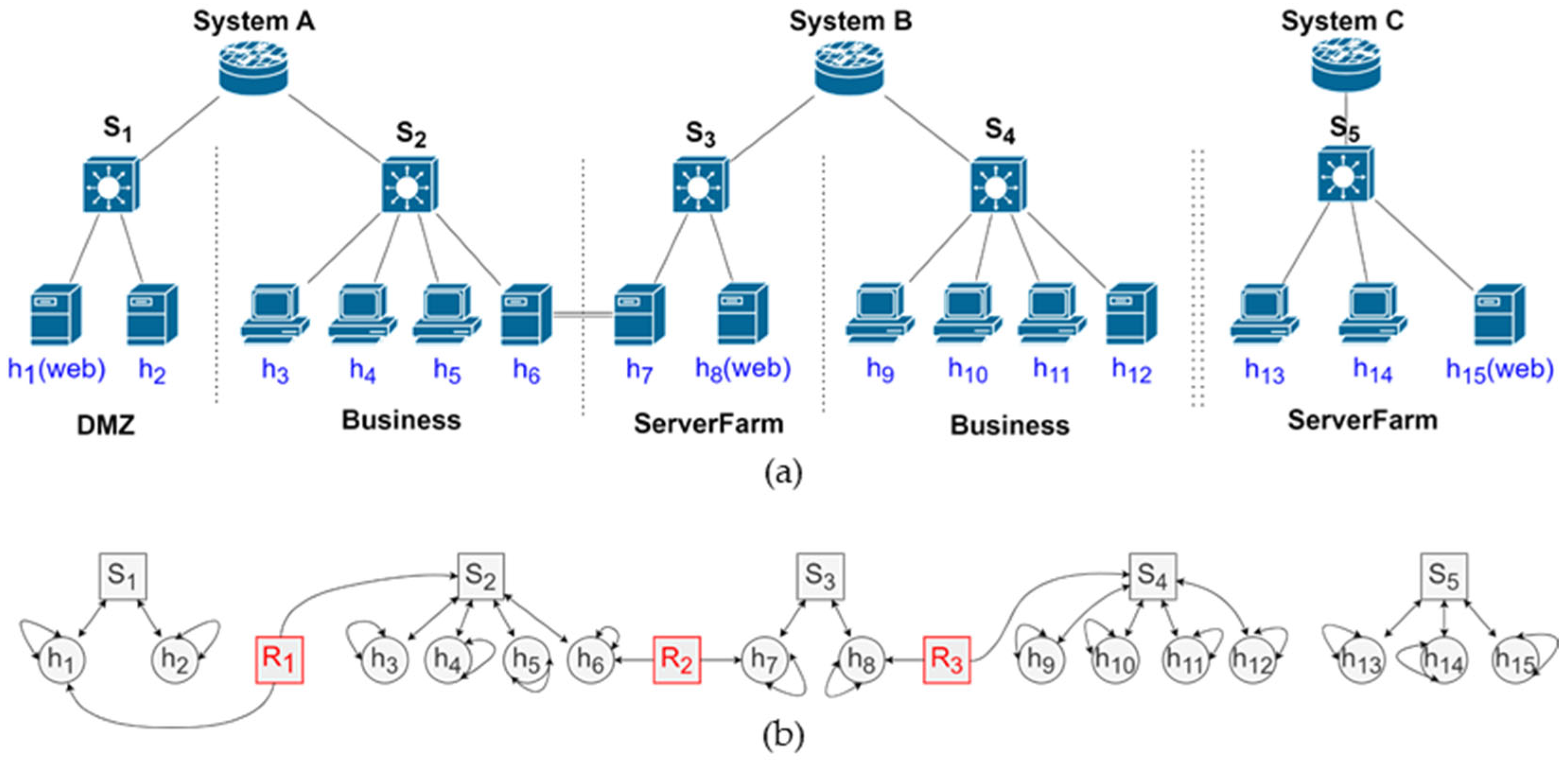
3.1. Low-Level Diffusion Model Based on MRM

3.1.1. Creation of Primitive Matrix

The diffusion process, which determines the reachability between assets in a network topology, applies graph theory, which models the pairwise relationships between objects to visualize the network topology as edges, which are connections between vertices in a graph. For visualization, the vertices of the graph are replaced by hosts in the network, and the connectivity between hosts is visualized as a square binary matrix, which is represented by a primitive matrix.

A binary matrix, also known as a logical matrix, relational matrix, or Boolean matrix, is a matrix that represents a binary relationship between a pair of finite sets, where the elements of the matrix are zero and one. In this study, we generate an $m\times m$ square binary matrix with as many columns and rows as vertices to visualise the connectivity of $m$ hosts in a network topology. The element value $a_{j,k}$ of the primitive matrix is represented as (0, 1) depending on whether host $h_j$ is connected to host $h_k$ or not, and the primitive matrix ($A^0$) is generated through the following conditions (Figure 3a).

$$a_{j,k}=\left\{\begin{array}{c}1, j=k \mathrm{or} j\to k\\ 0, \mathrm{otherwise} \end{array}\right.,a_{j,k}\in A^0$$

(1)

In this study, we assume that an attack is possible if host $h_j$ can reach host $h_k$ via a path based on the connectivity between hosts. Accordingly, as in Noel and Jajodia’s work [4], hosts placed in rows represent hosts that can be attacked by the connections between hosts (referred to as destinations) and hosts placed in columns represent hosts that can be attacked (referred to as sources).

3.1.2. Power of the Primitive Matrix

The powers of the primitive matrix $A^0$, which visualises the connectivity between hosts in a network, can be used to determine in how many steps each host can be reached, that is, the number of hops. $A^i$, which is calculated by raising $A^0$ to the power of $i$ times, means that each host at the source can reach the destination host via i intermediate hosts or in $i$+1 steps (the number of hops) [4]. The elements of $A^i$ are represented by $A^i$($a_{j,k})$, where a is the host, $i$ is the number of powers, j is the row, and k is the column. In other words, for $A^1$, a value of one for $A^1$($a_{j,k})$ means that it is reachable in two steps from the source host to the destination host via one host.

In this study, the primitive matrix $A^0$ power $A^i$ is performed through a Boolean product, as shown in Equation (2), and an element with a value of one ($A^i$($a_{j,k})$ = 1) represents i state changes from host $h_j$ to host $h_k$, i.e., through i intermediate hosts to reach host $h_k$. Here, Equation (2) means that the primitive matrix $A^0$ is a Boolean (binary) matrix and is raised to a power through the Boolean product, where ☉ is the Boolean product operator.

$$A^i=A^{i-1}\odot A^0$$

(2)

The matrix $A^i$($i\in N_0$), which is obtained by taking the powers of the primitive matrix $A^0$ (Figure 3a), reflects the direct connectivity of each host, as well as the indirect connectivity through intermediate hosts. The transitive closure matrix is a matrix consisting of reachability elements [11], as shown in Figure 3b, which are denoted with a one if a reachable path exists between vertices and a zero if it does not. We consider the Transitive Closure State to be a state in which further powers do not change the state of the matrix, i.e., there is no change in reachability. In other words, the powers of the primitive matrix for predicting the reachability of hosts at a given stage are described by the Transitive Closure State. A matrix that has reached transitive closure is represented by $A^n$, where $A^n$ is $A^n$($A^n\left(a_{j,k}\right)\in A^n,\left[0,1\right])$, and $A^{n+1}-A^n=0$. Accordingly, let $i\left(0\le i\le 1;n\in N_0\right)$ be the number of powers of the primitive matrix $A^0$ and the number of intermediate hosts before host $h_j$ reaches host $h_k$.

3.1.3. MRM-Based Analysis of the Diffusion Process

The matrix for each stage, computed through the powers of $A^0$, represents the reachability based on whether the hosts are connected or not at that stage, and summing the matrices for each stage, as shown in Equation (2), accumulates and represents a value (zero or one) that represents the reachability of each stage from the initial stage ($A^0$) to the transitive closed state ($A^n$) between hosts over all possible number of stages. Note that the sum of each Boolean-powered matrix is computed as an arithmetic sum, not a Boolean sum.

$$S={{\displaystyle \sum }}_{i=1}^{n+1}{A}^{i-1}$$

(3)

In the case of Equation (2), each element of $S$ is represented by S$\left(a_{j,k}\right)$, which is the accumulated value of reachability, and Equation (3) is performed to determine the reachability of the entire host and the number of steps by each element. The matrix representing the reachability of each step (hop) through Equation (3) is expressed as a Multi-Step Reachability Matrix (MRM) $R^n$, and the elements of $R^n$ are expressed as $R^n\left(a_{j,k}\right)$. In $R^n$, the total number of steps is n + 1 and the number of intermediate hosts is n. This makes it easy to identify whether host $h_j$ can reach $h_k$ from $R^n\left(a_{j,k}\right)$ and how many hops it takes to reach it.

$$R^n\left(a_{j,k}\right)=\left\{\begin{array}{c}\left\{M-S\left(a_{j,k}\right)\right\}+1, a_{j,k}\ne 0\\ 0, a_{j,k}=0\end{array}\right.$$

(4)

$M$ is the maximum value of $\mathrm{S}\left(a_{j,k}\right)$ according to Equation (2) given $\mathrm{m}$ hosts, expressed as $M=\max \left(\mathrm{S}\left(a_{1,1},a_{1,2}, \dots , a_{m,n}\right)\right)$. The diagonal element value of the MRM is zero $\left(a_{i,i}=0\right)$.

The MRM $R^4$ in Figure 4 represents the step-by-step reachability by summing from the primitive matrix $A^0$ to $A^4$ in five steps of transitive closure according to Equations (3) and (4), with the same color for elements with the same number of steps for ease of understanding. This makes it easy to see how many steps it takes for a host or threat event from the source host to reach a specific host (target) at the destination from a column perspective, and in how many steps a specific host or threat event from the source host can reach all hosts or targets at the destination from a row perspective. For example, column 6 of $R^4$ shows that $h_6$ can reach $h_2$ and $h_8$ in two hops with one intermediate host, and row 1 of $R^4$ shows that $h_1$ can reach all hosts in four hops.

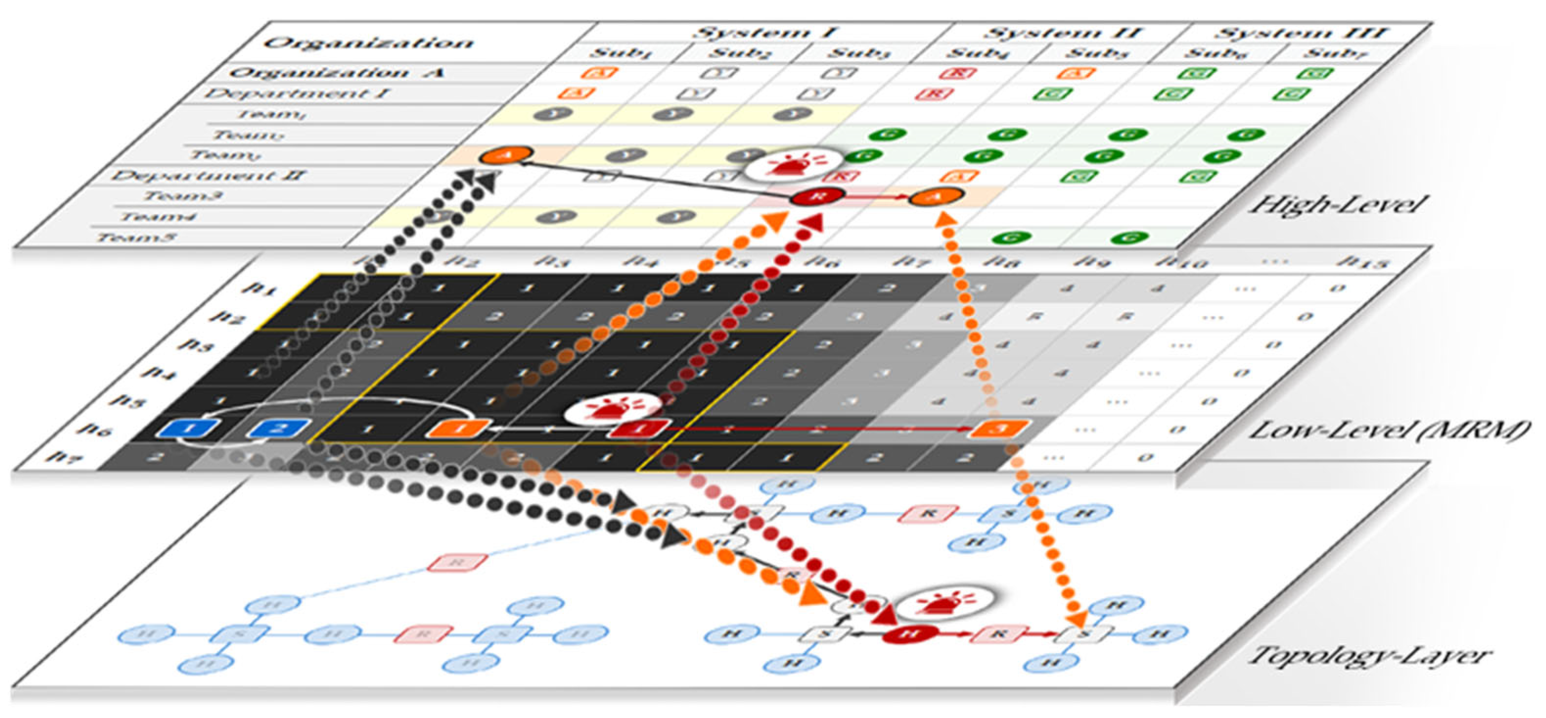
3.2. High-Level Abstraction for Strategic Decision Making

In large-scale networks, there are obvious limitations in the human perception of visualization means such as asset-level matrix tables, network topologies, and attack graphs. Even in attack graph research, the complexity of attack graphs often prevents them from being useful in practice, and methodologies have been proposed to better visualize them [12,13,14,15], while a high-level scenario graph (HSG) has also been proposed as a methodology for abstracting low-level threat alerts into attack campaigns [16]. In this paper, we propose an abstraction model for grouping assets into specific shapes that can reflect the reachability characteristics of the assets in an organization and support the decisions of top decision makers.

In this paper, we define the characteristics of the organizations (i.e., organizations, departments, network structures, systems, subnet groups, etc.) to which each host belongs in advance. Then, we use a method to selectively apply the results of the MRM to the corresponding organizations and calculate the distances (number of hops) between these corresponding organizations by allocating the results of the MRM to the corresponding organizations through calculations, just as we analyzed the relationships between assets (hosts) through the MRM2.

3.2.1. Relationship between Organization, System, and Host

In this paper, we define an organization as a set of assets with certain common conditions, and we also pay attention to the relationships between organizations in order to abstract them to the required level of abstraction to higher organizations. We present a taxonomy and structure that consider the characteristics of organizations to represent these organizations and their inter-organizational hierarchies, which can be created sequentially or simultaneously from the MRM to the required hierarchy, as shown in Figure 4.

First of all, to define the object (scope) of abstraction, we consider the concept of organization, which is an extension of the taxonomy commonly used in IT networks. The results are summarized as shown in

Table 2. Classification of groups.

Level	Group	Description	Remark
High-level	Organization	Organizational hierarchical relationship (i.e., company, department, team)	MRM2
	System	According to the classification criteria of the organization’s business network (i.e., Management Information System, group ware, factory automation system)
Low-level	Reachable Vector	Vector of connectivity and distance between hosts
Topology-layer	Subnet	Same subnet ID that the asset belongs to	Attack-Graph
	Host	According to asset classification criteria (including what the host owns, i.e., vulnerabilities, software, contents, etc.)

.

Each organization is composed of various sub-organizations (i.e., department, team, etc.). Each sub-organization carries out tasks through several systems according to the organization’s function, and these tasks are organically connected through reporting and direction hierarchies between the upper- and lower-level organizations of each system (Figure 5).

Each asset is connected through the connection information of the system and organization to which it belongs, and the system and organization are gradually abstracted according to the hierarchy. This provides basic information for the strategic judgment of the final decision maker from the perspective of an abstracted organization by connecting low-level asset status changes to high-level ones. The connection relationship between each host, system, and organization is shown in Figure 6.

3.2.2. Determination of Entry ($e{n}_i$) and Exit Nodes ($e{x}_i$) for Organization

As shown in Figure 7, the network of each organization consists of multiple assets, including an entry node ($e{n}_i$), which is a node that can receive data from the outside to the organization, and an exit node ($e{x}_i$), which is a node that transmits the organization’s data to an external adjacent organization. At this time, $e{n}_i$ and $e{x}_i$ have directionality. However, in an undirected graph, $e{n}_i$ and $e{x}_i$ have the same properties. That is, we call these nodes, which are both $e{n}_i$ and $e{x}_i$, connecting nodes.

In a network consisting of many organizations, the entry/exit nodes of a particular organization ($Organizatio{n}_k$) are determined in the primitive MRM $R^0$. In matrix $R^0$, the hosts that can depart from the hosts belonging to the corresponding organization are referred to as exit nodes ($e{x}_k$). If an element ($a_{i,j}$ with a value of ‘1’) that is a host with a connection to a neighboring organization other than the current organization is projected as a row in the initial matrix $A^0$, that host becomes an exit node, and if an element $a_{i,j}$ is projected as a column, that host becomes an entry node in the organization.

In other words, when $a_i, a_j$ are not elements in the same organization, this is constructed as shown in Equation (5).

$$A^0\left(a_{i,j}\right)=1 \to \left\{\begin{array}{c}{a}_i=e{x}_i, \exists a_i\in \left\{Origin organizatio{n}_i\right\} \\ a_j=e{n}_j, \exists a_j\in \left\{Destination organizatio{n}_j\right\}\end{array}\right.$$

(5)

In Figure 8, $h_{2,3}$ can start from host $h_2$ in Department I and reach host $h_3$ in Department II, i.e., host $h_2$ is the exit node ($e{x}_I$) of Department I and host $h_3$ is the entry node ($e{n}_{II}$) of Department II. Similarly, in $h_{5,7}$, host $h_5$ is the exit node ($e{x}_{II}$) of Department II and host $h_7$ is the entry node ($e{n}_{III}$) of Department III.

3.2.3. Calculating the Depth of Transmission (DoT) to Identify the Extent of Diffusion between Organizations

Each organization performs its function by configuring various topologies according to its unique mission and task, and the detected threat gradually affects each organization along the connection path of the hosts that compose the topology over time, ultimately reaching the organization that holds the target. Therefore, by defining the delivery depth of each organization in advance, the order of each organization affected by the threat and the distance between the organizations can be used to check the sequential degree of influence of each function that performs the mission and task.

In this paper, DoT is defined as the shortest distance (number of hops) from the entry nodes ($e{n}_k$) to the exit nodes ($e{x}_k$) of a specific organization in the MRM, as in Equation (6). Accordingly, when there are multiple entry nodes and exit nodes, the shortest distance becomes the Depth of Transmission (DoT) of the organization.

$$\mathrm{DoT}=\min \left\{e{x}_k-e{n}_k\right\},e{x}_k,e{x}_k\in Organizatio{n}_k$$

(6)

At this time, the depth of an organization that does not have a top-level organization (Root Organization) or entry/exit nodes (i.e., an organization that cannot transition to another organization, such as the initial starting organization or a dangling node) is defined as “0”.

In the transitive closure state of the network, the value of each element in the MRM represents the reachable distance between hosts. Therefore, in the MRM, each organization’s DoT (Depth of Transmission) is:

(i)

The row vector connecting the entry nodes ($e{n}_{II}$) $h_3$ and exit nodes ($e{x}_{II}$) $h_5$ of the assets beloning to the $Organizatio{n}_{II}$ described in the previous section as the output (${\overrightarrow{h}}_{3,5}=\left\{0, 1, 1\right\})$ from the MRM (Figure 8c).

(ii)

According to Equation (6), ${\mathrm{DoT}}_{II}=\min \left\{e{x}_{II}-e{n}_{II}\right\}=1-0=1$ can be obtained.

Expanding further, let us assume an organization with five departments, as shown in Figure 9a. Each department has various networks that fit its characteristics, but in this section, we only focus on the interfaces between departments. In Equations (5) and (6), each department calculates the DoT between departments and generates the MRM, as shown in Figure 9a. Then, we compare the results with Figure 9b, which does not consider the DoT.

We will explain specifically about Departments $D_3$, $D_2$, and $D_4$, although there are differences depending on whether the DoT is applied. First, in Figure 9b, which does not consider DoT, $D_3$ has the same distance of two to $D_2$ and $D_4$. This indicates that the degree of threat that occurs in $D_3$ is the same as that in $D_2$ and $D_4$ when considering network centrality. However, considering the DoT, the distance of $D_2$ changes to three due to the DoT of the intermediate department $D_1$. This means that $D_4$ is relatively closer to $D_3$, which means that it has a high importance and should be considered as a factor in the decision making of top decision makers.

DoT has many paths, even at the shortest or equal distance. However, we focus on the values of distances between organizations when the intrinsic values of the organizations are the same, rather than on the problem of interpreting different paths of the same distance. That is, it is assumed that organizations on many paths with the same distance have the same importance.

4. Interpreting Threat Alerts through MRM2

If we apply intrusion alerts to the MRM, as shown in Figure 10b, as in the work of Noel and Jajodia [4], we can interpret these intrusion alerts by plotting their locations on a matrix, as shown in Figure 10a. Based on the results of MRM $R^4\left(a_{3,k}\right)$, which places the asset $h_3$ where the threat event occurs in the center of the concentric circles ($i$ = 0) and the corresponding hosts in each power number ($i$) of the concentric circles as the depart (source) point, rearranging the assets, as shown in Figure 10a, can easily identify which path the threat is spreading through and at what speed. Furthermore, we can understand the spread of simultaneous intrusion alerts by creating a synthesis matrix.

In addition, based on the results of the generated MRM, as in Alertⓐ in Figure 10b, the fact that an intrusion alarm sounds in an area with an element value of zero in a transitive closure state can be used as a basis for judging that the intrusion alarm is false, as the intrusion alarm sounding in a host cannot be reached through any host according to the diffusion model of this study.

4.1. Calculating the Distance between the Entry Point and the Destination in Case of a Threat

By projecting the points in the reachable area where the intrusion alert is raised onto $R^n$, one can predict how many steps an attacker would need to take to reach the detected location to break in, how many steps (or hops) it would take to reach key assets in the network that are reachable from the host where the intrusion alert is raised, or how many steps (or hops) it would take to spread across the entire network.

If an intrusion detection alert originates from a specific host where both the source and destination are known, we can project it onto $R^n$ to see how many steps it took to reach it. For example, in Figure 10b, the intrusion alert from Alertⓑ indicates that the attacker originates from host $h_1$ and reaches $h_3$ in one step ($R^4\left(a_{1,3}\right)$ = 1) without making any intermediate host.

Furthermore, even if the source host, i.e., the location of the attacker, is unknown, if an intrusion detection alarm occurs on host $h_k$, the distance (step) between each source host (entry host) and $h_k$ can be calculated from the elemental value of the column where $h_k$ in $R^n$ corresponds ($R^n\left(a_{j,k}\right)$). As shown in Figure 11a, the distance (in steps) from which $h_3$ (k = 3) can be reached and the distance (in steps) to reach it is $R^4\left(a_{j,3}\right)$. In other words, $R^4\left(a_{j,3}\right)$ means that an attacker can start from hosts $h_1$, $h_4$, $h_5$, and $h_6$ and reach $h_3$ without making any stops, in one step ($R^4\left(a_{1,3}\right)=R^4\left(a_{4,3}\right)=R^4\left(a_{5,3}\right)=R^4\left(a_{6,3}\right)=1$), and $h_2$ and $h_7$ can be reached in two steps ($R^4\left(a_{2,3}\right)=R^4\left(a_{7,3}\right)=2$). We can see that $h_8$ can be reached in three steps ($R^4\left(a_{8,3}\right)$ = 3), and $h_9$, $h_{10}$, $h_{11}$, and $h_{12}$ can be reached in four steps ($R^4\left(a_{9,3}\right)=R^4\left(a_{10,3}\right)=R^4\left(a_{11,3}\right)=R^4\left(a_{12,3}\right)=4$) for $h_3$. We can also see that $h_{13}$, $h_{14}$ and $h_{15}$ are hosts that are unreachable from $h_3$ ($R^4\left(a_{13,3}\right)$, $R^4\left(a_{14,3}\right)$, $R^4\left(a_{15,3}\right)=0$) and, therefore, do not affect the intrusion alert.

In the same way, by projecting the alerts generated by the intrusion detected on host $h_j$ onto MRM $R^n$, we can predict the possible destinations that $h_j$ can reach and the distance (in steps) to each destination by the element value ($R^n\left(a_{j,k}\right)$) of the row to which $h_j$ corresponds. As shown in Figure 11b, the destinations (targets) that $h_3$ (j = 3) can reach and the distance (steps) required to reach them can be identified by $R^4\left(a_{3,k}\right)$. This indicates that $h_3$ can reach $h_1$, $h_4$, $h_5$, and $h_6$ in just one step (without any intermediate host), as represented by ($R^4\left(a_{3,1}\right)=R^4\left(a_{3,4}\right)=R^4\left(a_{3,5}\right)=R^4\left(a_{3,6}\right)=1$). It also shows that $h_3$ can reach $h_2$ and $h_7$ in two steps ($R^4\left(a_{3,2}\right)=R^4\left(a_{3,7}\right)=2$). $h_3$ can reach $h_8$ in three steps ($R^4\left(a_{3,8}\right)$ = 3) and $h_9$, $h_{10}$, $h_{11}$, and $h_{12}$ in four steps ($R^4\left(a_{3,9}\right)=R^4\left(a_{3,10}\right)=R^4\left(a_{3,11}\right)=R^4\left(a_{3,12}\right)=4$). Similarly, $h_3$ cannot reach $h_{13}$, $h_{14}$, and $h_{15}$ ($R^4\left(a_{3,14}\right)=R^4\left(a_{3,14}\right)=R^4\left(a_{3,15}\right)=0$), indicating that $h_{13}$, $h_{14}$, and $h_{15}$ are hosts not affected by the intrusion alert threat.

Additionally, by projecting and abstracting the host-based diffusion process analyzed at a low level to a high level, this can provide insight into which sub-organizations and tasks (functions) within the organization the threat originated from, how the threat diffused through various sub-organizations and tasks (functions), and the number of transitions required to impact other sub-organizations and operations. This information can contribute to the situational awareness of decision makers and help to establish defense priorities from the perspective of the entire organization.

4.2. Synthesize Multiple Intrusion Alerts within an Organization

As a network grows in size or threats targeting an unspecified number of people occur simultaneously in multiple places during a specific period, it becomes difficult to explain the impact on the network simply by analyzing the impacts of individual hosts. Therefore, it is necessary to comprehensively consider multiple threats. Therefore, in order to analyze intrusion alerts targeting multiple hosts that occur during a specific period, this study combines the source hosts of each alert point, generates a primitive composite matrix ${\widehat{A}}^0$ of those combinations, and performs exponentiation ${\widehat{A}}^l$ to explain the impacts of multiple intrusion alerts. To this end, the set of synthesized threats is set as an element ${\widehat{A}}^0\left(a_{j,k}\right)$ of the composite matrix, and the combination that reaches a transitive closed state in the smallest number of steps, i.e., can reach all hosts the fastest, is interpreted as the combination with the highest risk by calculating it according to Equations (2)–(4).

The primitive composite matrix ${\widehat{A}}^0$ is generated by performing a disjunction (1 = T, 0 = F) on the rows and columns of the hosts to be combined among the hosts that sound an intrusion alarm from the primitive matrix $A^0$, assuming that the hosts that the synthesized host group can reach will be the same and deleting the rows and columns of the hosts used in the combination. That is, when combining $l$ hosts among the hosts that sound an alarm in the $m\times m$ matrix $A^0$, ${\widehat{A}}^0$ becomes a $\left(m-l+1\right)\times \left(m-l+1\right)$ matrix, and when $h_j, h_k, \dots , h_l$ are the hosts to create the combination, the $\widehat{h}$ generated by synthesizing them is performed as in Equation (7), where ∨ is a disjunction operator. At this time, in order to synthesize the hosts that sound an intrusion alarm, the synthesis targets must exist in the same network, and they are not synthesized when they are in a state where they cannot reach each other, such as in mutually independent networks.

$$\widehat{h}=h_j\vee h_k\dots \vee h_l$$

(7)

The generation of a composite matrix of multiple threats is further explained in Section 5.

4.3. Assessment and Action of Threats

When newly recognized threat information or detected intrusion alerts occur, the likelihood of them acting as a threat is analyzed by considering the impact on the system. In this section, the level of threat is identified by considering the diffusion step between the intrusion alert and the asset, that is, the distance between the attacker and the defense asset, and the priority is provided.

Accordingly, the degree of the identified threat can be explained by the relationship between the importance of the assets of the target host and the host that can be penetrated (or the intrusion detected). Therefore, in this study, the degree of the threat to host $\mathrm{TH}\left(h_j\right)$ and the degree of the threat to the system that includes the threat $\mathrm{TS}\left(s_j\right)$ are expressed as in Equation (8). Therefore, it can be interpreted that the impact is greater for larger organizations with many hosts or organizations with many assets that are greatly affected by threats.

$$\begin{gathered} \mathrm{TH}\left(h_j\right)={\displaystyle \sum }_{k=1}^n\left(w_k\times P\left(h_k\right)\times Hc\left(\overline{h_j{h}_k}\right)\right) \\ (0\le w_k, P\left(h_k\right)\times Hc\left(\overline{h_j{h}_k}\right) \\ \mathrm{TS}\left(s_j\right)={\displaystyle \sum }_{j=1}^{n}TH\left(h_j\right), \left(h_j\in s_j\right) \end{gathered}$$

(8)

Here, $\mathrm{TH}\left(h_j\right)$ is the threat level of the threat source host $h_j$, $w_k$ is the threat weight of the target host $h_k$, $P\left(h_k\right)$ is the asset importance of the target host $h_k$, and $Hc(\overline{h_j{h}_k)}$ is the asset connectivity value from the threat source $h_j$ to the target asset $h_k$, which is calculated using closeness centrality ($C_c$) in this study. Additionally, we calculate the extent to which each asset affects the upper system through a weighted sum [17].

Accordingly, assuming that intrusion alarms sounded on all hosts in the sample network in Figure 2, the level of threat to these assets can be expressed as in

Table 3. Degree of threat in Figure 2.

$\mathbf{Host}\left({\mathit{h}}_{\mathit{j}}\right)$	$\mathit{R}{\mathit{d}}_{\mathit{m}\mathit{a}\mathit{x}}^4$ 1	$\mathit{R}{\mathit{d}}_{\mathit{s}\mathit{u}\mathit{m}}^4$ 2	TH	TS
$h_1$	4	27	0.423	4.786
$h_2$	5	37	0.305
$h_3$	4	28	0.407
$h_4$	4	28	0.407
$h_5$	4	28	0.407
$h_6$	3	22	0.524
$h_7$	3	22	0.478
$h_8$	4	24	0.367
$h_9$	5	31	0.367
$h_{10}$	5	31	0.367
$h_{11}$	5	31	0.367
$h_{12}$	5	31	0.367
$h_{13}$	1	3	0.666	1.998
$h_{14}$	1	3	0.666
$h_{15}$	1	3	0.666

¹$R{d}_{max}^n$: when there are n + 1 steps, the longest shortest path from $h_j$ to $h_k$ (the maximum value of the elements in the $h_j$ row). ² $R{d}_{sum}^n$: when there are n + 1 steps, the sum of the shortest paths (elements in the $h_j$ row) from $h_j$ to $h_k$.

below. At this time, the weight $w_k$ and importance $P\left(h_k\right)$ for each target asset are different depending on the organization and operator, so they are not considered in this study and are all set to one.

When a threat is identified that is not specific to the attacker’s location or is provided as information by external information, the attack surface with the external attacker is identified and prioritized. In order for an attacker to exploit a host of a specific system from the outside, the attack must be made through a connection surface between the system and the outside. For example, if a system has multiple external attack points, such as a web server or mail server, the system security manager must determine which connection point would pose a relatively high threat to the attacker when infiltrating.

In Figure 2, $h_1$ and $h_8$ are web servers, and these hosts can connect to external systems. Assuming that $h_{11}$ is the asset that the system security manager must defend first, that is, the asset with the highest asset importance P($h_{11}$), then $h_1$, which is one of the attack contact points, can reach $h_{11}$ in four steps through three intermediate hosts by $R^4$ in Figure 4, but $h_8$ can be reached in only one step (hop) without any intermediate hosts. Therefore, from the perspective of defending host $h_{11}$, $h_8$ can be said to be more important as an attack surface than $h_1$. Therefore, the system security manager can determine that they should pay attention to $h_8$ first.

4.4. Selecting the Optimal Point for Threat Avoidance

Based on $R^n$, we can find the hosts that can reach the transitive closure state the fastest and change their connection relationship to identify effective connection or blocking points. In MRM $R^4$ of Figure 11, excluding $h_{13}$, $h_{14}$, and $h_{15}$, which exist in independent networks and the same subnet group, the hosts that reach the transitive closure state the fastest are $h_6$ and $h_7$, and both hosts can reach all hosts in only three steps. In addition, when comparing the two hosts, $h_7$ can reach all hosts except $h_2$ in only two steps, but $h_6$ needs to go through three steps to reach a total of four hosts, $h_9–$~$h_{12}$. Therefore, if the importance of $h_2$ is not relatively high, it can be determined that blocking the connection of $h_7$ is more efficient than blocking all connections with $h_6$, $h_7$, and other hosts.

Accordingly, in this study, in order to understand the result of blocking the connection of $h_7$, the connection relationship with $h_6$ and $h_8$ that can be connected to $h_7$ in the primitive matrix $A^0$ was created by changing the values of $a_{6,7}$, $a_{7,6}$, $a_{7,8}$, and $a_{8,7}$ from 1 to 0, as shown in Figure 12a, then generating a modified primitive matrix ${\widehat{A}}^0$, and generating the MRM ${\widehat{R}}^1$ according to Equations (2)–(4). As a result, $h_7$ is in a transitive closure state in the second step (hop) through one intermediate host, as in ${\widehat{A}}^1$ of Figure 12b, so that $h_7$ is completely isolated from other hosts, $h_1–h_6$ cannot reach $h_7–h_{15}$, $h_8–h_{12}$ cannot reach $h_1–h_7$ and $h_{13}–h_{15}$, $h_{13}–h_{15}$ cannot reach $h_1–h_{12}$, and $h_7–h_{15}$ cannot reach any other hosts.

As seen above, the security officer of the network can find the combination of hosts that can spread the fastest and determine the priority of the hosts that should be prioritized for defense, and even if an intrusion has not occurred, if a host with many connections between hosts or an essential host for defense is selected, the diffusion process can be examined through each combination of hosts based on the hosts that can reach the hosts the fastest. This can be utilized for preventive activities in peacetime before an attack or intrusion alarm sounds. In addition, by applying a policy to change the network path between the attack surface, which is the external connection point, and the main protection target host through MRM analysis, which is the reaching stage between the attack surface and the main protection target host, that is, to increase $R^n$, the complexity of the attack can be increased, reducing the attack success rate, increasing the detection opportunity as the number of intermediate hosts increases, and applying a path that is advantageous to the defender who secures defense time.

5. Experimental Scenario Design and Results

5.1. Pre-Construct Organizational and Topological Information

Considering the organization of Company A, as shown in Table A1, the company is structured with a management department responsible for overall management, two sales branches with different physical locations for handling sales, and a factory responsible for manufacturing products. In total, there are three departments and six subordinate teams, each utilizing Management Information Systems (MISs), Enterprise Resource Planning (ERP) Systems, and Factory Automation (F.A) Systems. The factory operates on an isolated (independence) network with its own Factory Automation (F.A) System, separate from external connections. Additionally, each team is divided into 12 subnet groups, comprising a total of 48 assets. Each asset follows the relationship detailed in

Table A2. List of hosts and adjacency list.

Host	Adjacency List	Host	Adjacency List
$h_1$	-	$h_{25}$	$h_4$$, h_{10}$
$h_2$	-	$h_{26}$	-
$h_3$	$h_5$$, h_6$$, h_7$$, h_8$	$h_{27}$	$h_{29}$$, h_{30}$$, h_{31}$$, h_{32}$
$h_4$	$h_{10}$$, h_{17}$$, h_{25}$	$h_{28}$	-
$h_5$	$h_3$	$h_{29}$	$h_{27}$
$h_6$	$h_3$	$h_{30}$	$h_{27}$
$h_7$	$h_3$	$h_{31}$	$h_{27}$
$h_8$	$h_3$	$h_{32}$	$h_{27}$
$h_9$	-	$h_{33}$	$h_{12}$
$h_{10}$	$h_4$$, h_{25}$	$h_{34}$	-
$h_{11}$	$h_{13}$$, h_{14}$$, h_{15}$$, h_{16}$	$h_{35}$	$h_{37}$$, h_{38}$$, h_{39}$$, h_{40}$
$h_{12}$	$h_{33}$	$h_{36}$	-
$h_{13}$	$h_{11}$	$h_{37}$	$h_{35}$
$h_{14}$	$h_{11}$	$h_{38}$	$h_{35}$
$h_{15}$	$h_{11}$	$h_{39}$	$h_{35}$
$h_{16}$	$h_{11}$	$h_{40}$	$h_{35}$
$h_{17}$	$h_4$	$h_{41}$	-
$h_{18}$	-	$h_{42}$	-
$h_{19}$	$h_{21}$$, h_{22}$$, h_{23}$$, h_{24}$	$h_{43}$	$h_{45}$$, h_{46}$$, h_{47}$$, h_{48}$
$h_{20}$	-	$h_{44}$	-
$h_{21}$	$h_{19}$	$h_{45}$	$h_{43}$
$h_{22}$	$h_{19}$	$h_{46}$	$h_{43}$
$h_{23}$	$h_{19}$	$h_{47}$	$h_{43}$
$h_{24}$	$h_{19}$	$h_{48}$	$h_{43}$

, and the Network Topology’s Logical Reachability Map derived from this information can be represented as shown in Figure A1.

Before the occurrence of threats, pre-generated network information is regularly reviewed and updated to reflect changes such as the introduction of new assets, alterations in network policies, the addition of new security elements, and modifications to the organizational structure. By utilizing the information available before threat detection to create or update the MRM2 and then projecting any detected threats or obtained information onto the generated MRM2, it becomes possible to analyze the information and overcome the challenges associated with real-time pathfinding when a threat occurs.

Based on the above basic information, a primitive matrix $A^0$ is generated according to the condition of Equation (1) and a low-level MRM is generated as shown in Figure A2 after exponentiation, according to Equations (2)–(4), until the transitive closure state is reached. At this time, the exponentiation number ($i$) of the transitive closure state is seven.

The primitive matrix has values of zero and one; if the value is one, it is displayed in gray, and the hosts in the same subnet group are displayed with a bold border so that they can be identified as a fully connected group.

Using the MRM generated based on the pre-configuration information of each asset and system team, a high-level abstraction matrix is generated for each sub-organization and system unit, as shown in Figure 13. Currently, no threats have occurred, and each system and organization is in a stable state.

5.2. Threat-Scenario-Based Impact Analysis

In order to generate a threat scenario, this paper assumes that an intrusion is detected on the control server ($h_{27}$) of Subnet Group 7 of Sales Department Branch 2 and the client ($h_{37}$) of Factory Department Materials Team Subnet Group 10. Using the previously generated MRM2, a new MRM is generated through multi-threat synthesis and a low-/high-level threat analysis is performed.

Diffusion Impact Analysis for Primary Actions in Threat Alerts

When intrusion alarms sound simultaneously on two hosts ($h_{27}$, $h_{37}$) of Company A, the hosts $h_{27}$ and $h_{37}$ are synthesized into a new host Group $\widehat{h}1$ from the primitive matrix $A^0$, as shown in Figure 14a, and the initial synthesized matrix ${\widehat{A}}^0$ is generated, as shown in Figure 14b ($\widehat{h}1=h_{27}\vee h_{37}$). By generating the MRM of ${\widehat{R}}^6$ according to Equations (2)–(4), we can determine to what extent the threat can spread from the host where the threat occurred to all hosts of Company A.

As a result of the exponentiation of the newly synthesized 47 × 47 initial composite matrix, ${\widehat{A}}^0$ reaches a transitive closure state (${\widehat{A}}^6={\widehat{R}}^6$) in step 7, and as shown in Figure A3, $\hat{\mathrm{h}}1$ ($h_{27}\vee h_{37})$ reaches a transitive closure state that any host can reach in just six steps, so it can reach all hosts in the network except for the hosts in the independent network (Company A’s factory). Through this, we confirm that the diffusion speed is faster than that of the original 48 × 48 matrix $A^0$, which reaches a transitive closure state in step 8 for the individual hosts $h_{27}$ and $h_{37}$, as shown in

Table 4. Comparison of results before and after applying composite matrix (${\widehat{A}}^6$) of multiple threats to Company A’s network ($h_1–h_{40}$).

MRM Matrix		${\mathit{A}}^7$	${\widehat{\mathit{A}}}^6$	Box-and-Whisker Diagram
Threat host		$h_{27}, h_{37}$	$\widehat{h}1=h_{27}\vee h_{37}$
Number of hosts		40	39
$\mathrm{Number} \mathrm{of} i\left(step\right)$		7(8)	6(7)
$R{d}_{max}^i$	Min	4	4
	Ave	6.58	5.74
	StDev	1.03	0.82
$R{d}_{sum}^i$	Min	105	94
	Ave	160.9	138.87
	StDev	28.10	21.87
View Details		Figure A2	Figure A3

. (For details of the generated MRM, see Figure A2 and Figure A3.)

If the MRM generated at this time is projected into a high-level abstraction matrix, it is as shown in Figure 15. Company A’s F.A System, which is configured as an independent network, is not affected by the threat, but the threat generated from the ServerFarm control server ($h_{27}$) of Branch 2 in the Sales Department immediately and directly affects all clients in subnet group 8 of the adjacent Branch 2 and the MIS/Purchase Team ServerFarm of the Management Department, and then gradually affects the entire MIS system.

In addition, it can be confirmed that the threat detected from the client of Material Team Subnet Group 10 in the Factory Department directly affects the ServerFarm of the same team Subnet Group 9, and gradually affects all ERP systems linked to Subnet Group 9. Also, we can see that the Purchase Team of the Management Department, which operates the ERP System, is affected by threats from both $h_{27}$ and $h_{37}$, and here, considering the DoT, we can say that it is more affected by the threat spread from the Branch 2 Team of the Sales Department, which has a relatively short DoT, than the threat spread from the Materials Team of the Factory Department.

Accordingly, the top decision maker can easily understand the impact of the threat on the organizational function under the priority of organizational operation, and can plan count measures according to the priority that can take appropriate measures according to the speed of diffusion.

Detected threats, over time, may propagate through various activities and impact each host. As these hosts are affected, the functionality of each system may gradually deteriorate, leading to potential risks.

As shown in

Table 5. Impacts of threat diffusion on hosts and systems.

	Hop	Affected Host ID		Affected System 1
Impact				MIS System			ERP System		Total 2
				MGMT.	Salse		MGMT.	Factory
				MIS	Branch 1	Branch 2	Purchase	Material
0		27	37	0/8	0/8	1/8	0/8	1/8	2/40
1		25, 26, 28, 29, 30, 31, 32	35, 38, 39, 40	0/8	0/8	8/8	0/8	5/8	13/40
2		4, 10	33, 34, 36	1/8	0/8	8/8	1/8	8/8	18/40
3		1, 2, 3, 9, 11, 12, 13, 17	12	4/8	1/8	8/8	4/8	8/8	25/40
4		5, 6, 7, 8, 18, 19, 20	13, 14, 15, 16	8/8	4/8	8/8	8/8	8/8	36/40
5		21, 22, 23, 24	-	8/8	8/8	8/8	8/8	8/8	40/40

¹ Number of affected hosts/Total number of hosts. ² Exclude F.A systems that are not threatened by independent networks.

, the threat that occurs starts from the same subnet group and exit node as it passes through the hop, and approaches the adjacent network through the entry node. A threat that enters through the entry node acts through the network in the same way. If this threat is carried out for the purpose of reconnaissance activities, it can acquire the path information of the organization network in advance. If it is explained without considering the service characteristics between the server and the client in the case of a specific malware, it can gradually reduce the availability of the organization by contaminating the host through this diffusion path. As shown in Table 5, in the case of malware that progresses by contaminating the host at each intermediate host, it can be seen that the function of Branch 2, which is close to the threat, will start to be paralyzed depending on the hop, and gradually, the function of the Material Team of the Factory. After five hops, all functions except for the F.A System of the Factory, which is a network composed of a single network, can be paralyzed.

5.3. Multi-Threat Assessment Considering Defensive Effectiveness

The diffusion of intrusion alerts triggered simultaneously across multiple hosts over a certain period represents a worst-case scenario for defenders. To address this, it is essential to analyze the impact by considering the most critical combinations of intrusion alerts and prioritize responses accordingly. This study proposes a method for generating the worst-case host combinations with the highest potential for rapid spread (i.e., those that can reach network hosts the quickest), based on the locations where simultaneous intrusion alerts were triggered. This method aims to aid in attack path prediction and defense strategies.

In order to identify which combination of assets exposed to a specific threat or assets that have triggered an intrusion alert shows the fastest diffusion in the target network and which combination should be prioritized to slow down the spread, the primitive matrix $A^0$ was created based on a network of 48 hosts of Company A, as shown in Figure 14a, and then the MRM $R^7$ was created, as shown in Figure A2. Then, assuming that three intrusion alerts were triggered, three random hosts ($h_4$,$h_{10}$, and $h_{33}$) that generated intrusion alerts were selected, and their effects were analyzed. First, the combinations of two or more hosts that can be generated with these three hosts were selected as $h_4\vee h_{10}\vee h_{33}=\widehat{h}1\left(B^0\right)$, $h_4\vee h_{10}=\widehat{h}2\left(C^0\right)$, $h_4\vee h_{33}=\widehat{h}3\left(D^0\right)$, and $h_{10}\vee h_{33}=\widehat{h}4(E^0)$, and based on these, a total of four initial composite matrices were generated and compared through the MRM. The results are shown in

Table 6. Results of composite host $\widehat{h}1, \widehat{h}2, \widehat{h}3, \widehat{h}4$ analysis using MRM.

MRM	Number of Hosts	$\mathbf{Number} \mathbf{of} \mathit{i}\left(\mathit{h}\mathit{o}\mathit{p}\right)$	$\mathit{R}{\mathit{d}}_{\mathit{m}\mathit{a}\mathit{x}}^{\mathit{i}}$			$\mathit{R}{\mathit{d}}_{\mathit{s}\mathit{u}\mathit{m}}^{\mathit{i}}$
			Min	Ave	StDev	Min	Ave	StDev
$A^7$	40	7(8)	4	6.58	1.03	105	160.9	28.10
$\widehat{h}1\left(B^5\right)=h_4\vee h_{10}\vee h_{33}$	38	5(6)	3	4.87	0.78	72	123.63	21.36
$\widehat{h}2\left(C^6\right)=h_4\vee h_{10}$	39	6(7)	4	5.85	0.99	88	147.31	21.30
$\widehat{h}3\left(D^5\right)=h_4\vee h_{33}$	39	5(6)	3	5.00	0.83	81	133.44	22.84
$\widehat{h}4(E^5)=h_{10}\vee h_{33}$	39	5(6)	3	5.00	0.83	81	133.44	22.84

.

In conclusion, the MRM analysis results generated through the newly generated initial composite matrix showed that $\widehat{h}1$, which synthesized all three, and $\widehat{h}3$ and $\widehat{h}4$, which synthesized two, had the lowest hop count of six hops until the transitive closure state. In other words, $\widehat{h}1$, $\widehat{h}3$, and $\widehat{h}4$ could reach all hosts through five intermediate hosts, so they were evaluated to have the highest threat level, and compared to the case where they were not synthesized, i.e., $A^0$, it was found that there was a difference of two hops.

Also, the combinations of hosts that can infect a specific network the fastest were $h_4\vee h_{10}\vee h_{33}=\widehat{h}1\left(B^0\right)$, and $h_4\vee h_{33}=\widehat{h}3\left(D^0\right)$, $h_{10}\widehat{h}4(E^0)$, $\widehat{h}3\left(D^0\right)$, and $\widehat{h}4(E^0)$ had the same number of stages as $\widehat{h}1\left(B^0\right)$, but diffused through two intermediate hosts. As shown in Table 6, this is an advantageous factor for attackers, because it can reach the most hosts the fastest while reducing the attack cost, which means that we can conclude that the hosts that the defender should be interested in are of a high priority. Even without specifying a specific target, as shown in these results, we can determine which host in the network can reach the most hosts the fastest, that is, which combination of hosts can affect the entire system the fastest.

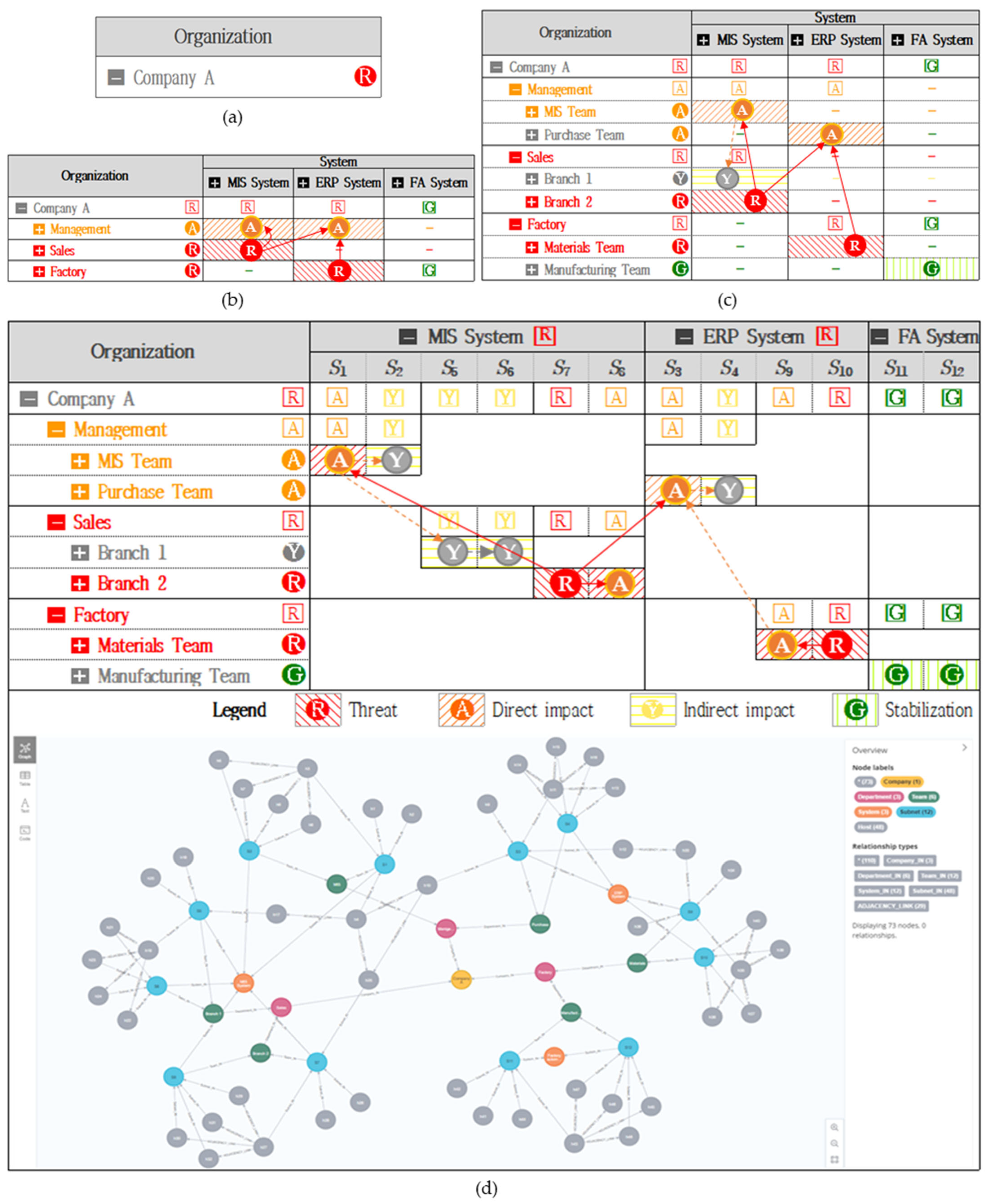
5.4. High-Level Abstraction for Strategic Decision Making

In the previous section, external or detected threats were projected into the MRM and analyzed at the asset level, taking into account the spread path, distance between assets, and priority of assets. In addition, the impact of the threat on the organization was abstracted to a high level to understand the ultimate impact of the threat on the organization, its impact on the organization’s objectives and mission, the order in which it affected subordinate organizations and functions for the decision making by top decision makers, and the order or priority in which it should be acted upon. The impact of the threat on the organization was expressed in an abstraction matrix, as shown in Figure 16.

As shown in Figure 16, the abstraction matrix provides a key means for intuitively scaling up or down to granular organizational components (Company, Department, Team, System, Subsystem, Subnet Group, and even Host) to match the interests of a C-level decision maker while preserving the MRM results. This allows one to see how threats are impacting each department or system and where they are prioritized for exposure and business impact. One can also understand the business criticality of each organizational function, which can be difficult for security personnel to grasp, identify key functions that need to be protected first, and strategically prioritize actions.

6. Discussion and Limitations

Previous studies have been conducted on calculating the distances between assets using a multi-level reachability matrix [4], on the impact of changes in the characteristics of assets on the mission or tasks of a specific organization [17,18,19], and on expressing corresponding threats as a higher-level model such as the kill chain [13]. However, this has not been explained from the perspective of organizations, which are the subjects that accomplish the mission or task and are the targets of kill chains. We extended the distances between assets to the relationship between low-level hosts and high-level organizations. We also grouped and hierarchized organizations, and presented methods for expressing the horizontal distances between organizations and expressions between the upper and lower organizations. Through this, the impact of threat diffusion between assets was expressed as the distance between organizations. It was presented as an additional consideration for not only security officers, but also top decision makers and organizational managers when establishing a Course of Action (COA) against cyber threats based on an organization’s goals.

However, in this paper, we did not discuss, in depth, the importance of assets or the importance of the organization itself. A simple quantification method was applied to allow for relative comparisons between systems, assuming that the more critical a system’s hosts that are affected by a threat, the greater the impact on the system [17]. Although this simplified methodology can account for differences in relative comparisons between systems, it has some limitations, in that it fails to take into account the complex and diverse characteristics of threats, hosts, and systems, and this is an area that requires further research. Furthermore, we focus on the relevance to organizations based on intelligence, which is the result of analyzing information collected from these tools, and topology information collected in advance, rather than correlations with various tools such as SIME (Security Information and Event Management) or SOAR (Security Orchestration, Automation, and Response). Therefore, its application to time-sensitive dynamic environments is limited. Additional research is also needed to take this into account.

7. Conclusions

This study presented the MRM2 approach, which is based on a multi-level reachability matrix for evaluating and analyzing multiple threats. The MRM2 describes the low-level, host-level threat propagation process and presents a methodology for determining the mitigation priority of threats based on this, and for compositing multiple threats that can occur in an organization to determine their impacts on the internal network. We preserve the low-level results by expanding the connectivity of assets, while adding to the traditional technology-centric perspective to provide a new high-level decision aid to assist organizational-level decision makers in making strategic judgments. This enables top-level decision makers to intuitively understand the impacts of cyber threats on each component of the organization downstream and share with their counterparts a high-level defense objective that considers the organization, mission, and functional aspects of the threat, rather than individual threats, to prioritize threat avoidance. This is expected to enable defense measures that reflect the intentions of top decision makers, not just technical considerations. In addition, by applying abstraction techniques that can be scaled up and down, it provides flexibility for situational awareness that can be applied to the size of the organization, decision makers in lower-level organizations, and security personnel who are delegated to make decisions. It will also contribute to the prioritization of defensive measures from the perspective of the entire organization.

Future research will further supplement the abstraction level by studying the quantitative contributions of assets to organizations, tasks, and functions, and building a large-scale test data set to enable the application of desired situational awareness, even in large-scale networks.

References

1. Kyle, I.; Lippmann, R.; Piwowarski, K. Practical attack graph generation for network defense. In Proceedings of the 2006 22nd Annual Computer Security Applications Conference (ACSAC’06), Miami Beach, FL, USA, 11–15 December 2006; pp. 121–130. [Google Scholar]
2. Misra, S.; Obaidat, M.S.; Bagchi, A.; Bhatt, R.; Ghosh, S. Attack graph generation with infused fuzzy clustering. In Proceedings of the International Conference on Security and Cryptography, SCITEPRESS, Milan, Italy, 7–10 July 2009; Volume 1. [Google Scholar]
3. Tao, L.; Chen, D.; Song, R. Measure large scale network security using adjacency matrix attack graphs. In Proceedings of the 2010 5th International Conference on Future Information Technology, Busan, Republic of Korea, 21–23 May 2010; pp. 1–8. [Google Scholar]
4. Steven, N.; Jajodia, S. Understanding complex network attack graphs through clustered adjacency matrices. In Proceedings of the 21st Annual Computer Security Applications Conference (ACSAC’05), Tucson, AZ, USA, 5–9 December 2005; pp. 10–169. [Google Scholar]
5. Xie, A.; Tang, C.; Gui, N.; Cai, Z.; Hu, J.B.; Chen, Z. An adjacency matrixes-based model for network security analysis. In Proceedings of the 2010 IEEE International Conference on Communications, Cape Town, South Africa, 23–27 May 2010; pp. 1–8. [Google Scholar]
6. Kim, K.-J.; Oh, S.-H.; Lee, D.-H.; Oh, H.-R.; Lee, J.-S.; Shin, D.-K. A research on cyber target importance ranking using PageRank algorithm. J. Korean Soc. Internet Inf. 2021, 22, 115–127. [Google Scholar]
7. Kertzner, P.; Carter, C.; Hahn, A. Crown Jewels Anaysis: For Industrial Control Systems; MITRE: McLean, VA, USA, 2022. [Google Scholar]
8. Lim, N.-K. A Study on Efficient Critical Cyber Asset Identification Methods for All Domain Operations. J. Mil. Sci. Res. 2023, 74, 127–147. [Google Scholar]
9. Kim, A.; Kang, M.H.; Luo, J.Z.; Velasquez, A. A framework for event prioritization in cyber network defense. 2014. Available online: https://apps.dtic.mil/sti/citations/ADA608707 (accessed on 29 September 2024).
10. Rodrigues, F.A. Network centrality: An introduction. In A Mathematical Modeling Approach from Nonlinear Dynamics to Complex Systems; Springer: Cham, Switzerland, 2019; pp. 177–196. [Google Scholar]
11. Tripathy, A. Transitive Closure of a Graph using Graph Powering & further optimization by Euler’s Fast Powering Algorithm. Int. J. Sci. Res. 2021, 10, 869–873. [Google Scholar]
12. Noel, S.; Jajodia, S. Managing attack graph complexity through visual hierarchical aggregation. In VizSEC/DMSEC ’04: Proceedings of the 2004 ACM workshop on Visualization and Data Mining for Computer Security; ACM Press: New York, NY, USA, 2004; pp. 109–118. [Google Scholar]
13. Noel, S.; Jacobs, M.; Kalapa, P.; Jajodia, S. Multiple Coordinated Views for Network Attack Graphs. In Proceedings of the IEEE Workshop on Visualization for Computer Security (VizSEC 2005), Minneapolis, MN, USA, 26 October 2005. [Google Scholar]
14. Lippmann, R.; Williams, L.; Ingols, K. An Interactive Attack Graph Cascade and Reachability Display; IEEE Workshop on Visualization for Computer Security (VizSEC 2007); Springer: Berlin/Heidelberg, Germany, 2007. [Google Scholar]
15. Homer, J.; Varikuti, A.; Ou, X.; McQueen, M.A. Improving Attack Graph Visualization through Data Reduction and Attack Grouping. In Proceedings of the International Workshop on Visualization for Computer Security, Cambridge, MA, USA, 15 September 2008; pp. 68–79. [Google Scholar]
16. Milajerdi, S.M.; Gjomemo, R.; Eshete, B.; Sekar, R.; Venkatakrishnan, V.N. Holmes: Real-time apt detection through correlation of suspicious information flows. In Proceedings of the 2019 IEEE Symposium on Security and Privacy (SP), San Francisco, CA, USA, 19–23 May 2019. [Google Scholar]
17. Jang, J.; Kim, K.; Yoon, S.; Lee, S.; Ahn, M.; Shin, D. Mission impact analysis by measuring the effect on physical combat operations associated with cyber asset damage. IEEE Access 2023, 11, 45113–45128. [Google Scholar] [CrossRef]
18. Musman, S.; Temin, A.; Tanner, M.; Fox, D.; Pridemore, B. Evaluatingthe Impact of Cyber Attacks on Missions. In Proceedings of the 5th International Conference of Information Warfare and Security, Dayton, OH, USA, 8–9 April 2010. [Google Scholar]
19. Noel, S.; Ludwig, J.; Jain, P.; Johnson, D.; Thomas, R.K.; McFarland, J.; King, B.; Webster, S.; Tello, B. Analyzing mission impacts of cyber actions (AMICA). In Proceedings of the NATO IST-128 Workshop on Cyber Attack Detection, Forensics and Attribution for Assessment of Mission Impact, Istanbul, Turkey, 15–17 June 2015. [Google Scholar]
Figure 1. MRM2 architecture.
Electronics 13 03921 g001
Figure 2. Sample network with 15 hosts and 5 subnet groups: (a) topology map of sample network and (b) reachability map of sample network.
Electronics 13 03921 g002
Figure 3. Generating the primitive matrix and the transitive closed-state matrix from the sample network(Yellow box means same subnet group and Gray cells represent reachability): (a) the primitive matrix A 0 and (b) transitive closed-state ( i = 4) matrix A 4 .
Electronics 13 03921 g003
Figure 4. Examples generated via MRM during R 4 .
Electronics 13 03921 g004
Figure 5. Organic connection with the organization and its components and systems: (a) the connection between organization–department–team–system–host and (b) an abstract matrix of (a).
Electronics 13 03921 g005
Figure 6. Interfaces between organization, system, subnet group, and host.
Electronics 13 03921 g006
Figure 7. Network model of departments I and N within company A: (a) directed graph and (b) undirected graph.
Electronics 13 03921 g007
Figure 8. Identifying the entry and exit nodes of Department II in the example network: (a) network topology graph; (b) finding entry and exit nodes in the adjacency matrix of company A; and (c) generating MRM.
Electronics 13 03921 g008
Figure 9. Calculating DoT from MRM of Sample Network: (a) MRM without considering DoT between departments; (b) MRM considering DoT between departments.
Electronics 13 03921 g009
Figure 10. Verifying the location and authenticity of the intrusion alerts: (a) visualization of R 4 and (b) intrusion alerts on R 4 .
Electronics 13 03921 g010
Figure 11. Interpreting h 3 in MRM R 4 : (a) R 4 a j , 3 : Source → h 3 and (b) R 4 a 3 , k :   h 3 Destination .
Electronics 13 03921 g011
Figure 12. Comparison results of A ^ 0 and A ^ 1 R ^ 1 : (a) modified primitive matrix A ^ 0 and (b) MRM A ^ 1 R ^ 1 .
Electronics 13 03921 g012
Figure 13. Abstraction matrix of company A.
Electronics 13 03921 g013
Figure 14. Primitive matrix and primitive composite matrix when a threat alert occurs in h 27 and h 37 : (a) primitive matrix A 0 and (b) primitive composite matrix A ^ 0 .
Electronics 13 03921 g014
Figure 15. Comparison and high-level abstraction matrix of threats from hosts h 27 and h 37 .
Electronics 13 03921 g015
Figure 16. Extension of and reduction in the abstraction matrix: (a) overall status of an organization; (b) status of threat impact by department and system within the organization; (c) status of threat impact by department, team, and system within the organization; and (d) status of threat impact by department, team, system, and subnet group within the organization.
Electronics 13 03921 g016