Abstract
This paper proposes a novel adaptive law that uses a quasi-convex function and a novel sliding variable in an adaptive sliding mode control (ASMC) scheme for robot manipulators. Since the dynamic equations of robot manipulators inevitably include model uncertainties and disturbances, time-delay estimation (TDE) errors occur when using the time-delay control (TDC) approach. Further, the ASMC method used to compensate for TDE errors naturally causes a chattering phenomenon. To improve tracking performance while reducing or maintaining chattering, this paper proposes an adaptive law based on a quasi-convex function that is convex at the origin and concave at the gain switching point, respectively. We also adopt a novel sliding variable that uses previously sampled tracking errors and their time derivatives. Further, this paper proves that the sliding variable of the robot manipulator controlled by the proposed ASMC satisfies uniformly ultimately bounded stability. The simulation and experimental results illustrate the effectiveness of the proposed methods in terms of tracking performance.
1. Introduction
Robot manipulators are used extensively across various industrial and academic fields, such as in manufacturing factories [] and medical facilities [,], where accurate and detailed manipulations are needed. To achieve high-precision control of robot manipulators, uncertain parameters, such as unknown disturbances, time-varying parameters, nonlinearities, and model uncertainties, need to be handled effectively; otherwise, they can degrade the control performance or cause instability in the manipulator systems [,]. To tackle this issue, many robust control methodologies, including backstepping control [], neural network (NN)-based control [,], fuzzy control [], time-delay control (TDC) [,], and sliding mode control (SMC) [,,], have been proposed.
TDC has proven to be an efficient control method when exact information about system dynamics is unknown since it recursively predicts uncertain parameters by using previously sampled angular acceleration and input torque [,]. Due to such a recursive structure of the TDC and computational limitations on hardware, time-delay estimation (TDE) errors are a natural result of using the TDC scheme. If the sampling interval is small enough to be considered zero, the TDE error can be ignored []. However, it is hard to satisfy this condition in real-world dynamic systems. To compensate for TDE errors and improve the tracking performance of robot manipulators, SMC schemes have been used simultaneously with TDC [,].
SMC is a robust control method that has numerous advantages such as a fast response, low computation, and a simple implementation []. Based on the Lyapunov theorem, this method uses a discontinuous control input [] that forces a sliding variable to converge to a sliding surface, where the sliding variable is equal to zero. On the sliding surface, the sliding variable is equal to an error dynamic equation and, in turn, the tracking error also converges to zero. To reduce model uncertainties, nominal parts of system dynamics [,] or TDC schemes [,] have been simultaneously utilized with SMC schemes. In this case, to guarantee that the sliding variable lies on the sliding surface, the SMC gain must be larger than the upper bound of the overall uncertainties and disturbances. However, it is hard to obtain what such upper bounds are in practice and, thus, the SMC gain is chosen to be sufficiently large to suppress any potential uncertainties and disturbances. Although large SMC gain may improve tracking performance in areas such as convergence times and tracking errors, an excessively large SMC gain combined with the discontinuous input structure induces high-frequency oscillations, also known as chattering, in the control input. It is well known that chattering induces crucial problems in many dynamic systems such as the wear of mechanical parts or heat losses from electrical parts. Therefore, to improve tracking performance while reducing or maintaining chattering, an adaptive sliding mode control (ASMC) scheme, which dynamically adjusts the SMC gain without prior knowledge on the upper bound of the uncertainties, has been proposed [,,,,].
The adaptive laws in ASMC schemes increase the control gain until the sliding variable reaches the sliding surface. In real SMC schemes, however, the control gain keeps increasing since the sliding variable cannot stay at the origin due to external disturbances, model uncertainties, and limitations on a sampling interval, which causes a control gain overestimation problem [,]. It has been noted that excessively large SMC gains near the sliding surface can enhance chattering. Therefore, as shown in Ref. [], ideal SMC, which forces the sliding variable to remain in the sliding surface, cannot be established. Instead, ASMC schemes in the literature [,,] force the sliding variable to converge in a vicinity of the sliding surface. Further, to improve tracking performance while reducing or maintaining chattering, the ASMC gain switches between two adaptive laws, which increase or decrease the control gain at predefined times or according to the domain of the sliding variables []. In Ref. [], a barrier function-based ASMC, which decreases the control gain near the sliding surface according to a convex function called a barrier function, is proposed. The barrier function used in this approach has an infinite value at the gain switching point to force the sliding variable to remain close to the sliding surface. However, such an infinite gain induces severe problems such as gain saturation and abrupt torque changes in real dynamic systems. To deal with this issue, Ref. [] additionally defines an upper threshold for the barrier function and proposes a modified barrier function-based adaptive law. Unfortunately, since this approach switches gain according to a predefined convergence time, conservatism exists in choosing the predefined time parameter. Typically, function-based adaptive laws [,] use convex functions to reduce the control gain to almost zero near the sliding surface. Thus, the control gain obtained from these methods rapidly decreases in the vicinity of the sliding surface. In other words, when the sliding variable diverges from the origin, these approaches rapidly increase the control gain, which can contribute to the chattering phenomenon.
Motivated by the above observations, we propose a novel adaptive law that uses a quasi-convex function [] and a novel sliding variable in an ASMC scheme with the goal of improving tracking performance while reducing or maintaining chattering. To the best of the authors’ knowledge, quasi-convex functions have not been used in the ASMC schemes. Since a quasi-convex function can contain both convex and concave parts, the proposed adaptive law is convex at the origin and concave at the gain switching point with respect to a sliding variable. We also propose a novel sliding variable that additionally uses previously sampled tracking errors and their time derivatives. This paper proves that the sliding variable of the robot manipulator controlled by the proposed ASMC satisfies uniformly ultimately bounded (UUB) stability. The simulation and experimental results illustrate the effectiveness of the proposed methods in terms of tracking performance.
Notation: and represent the Euclidean norm and the infinity norm, respectively. represents the sign function. is the set of n-dimensional vectors. is the set of real matrices. stands for a diagonal matrix. I is the identity matrix with appropriate dimensions. For a given positive scalar L, is the time-delayed value of . denote a vector and its elements.
2. Preliminaries
This section presents an existing definition, a lemma, and a system formulation to explain the proposed ASMC.
Definition 1
([]). The variable is uniformly ultimately bounded (UUB) with ultimate bound b if there exist positive constants b and c, independent of , and for every , there is , independent of , such that
Lemma 1
([]). A twice-differentiable function of a single variable x defined on the interval I is
- Concave if and only if for all x in the interior of I.
- Convex if and only if for all x in the interior of I.
A dynamic equation for a robot manipulator with n degrees of freedom (DOF) is expressed as follows:
where ∈ are the angle, angular velocity, and acceleration vector of each manipulator joint, respectively. are the inertia matrix and the Coriolis matrix, respectively. are the gravitational force vector, the friction force vector, and the input torque vector of each manipulator joint, respectively. The dynamic Equation (2) can be reformulated as follows:
where is a positive-definite diagonal matrix and . Due to the time-varying and nonlinear nature of the function , it is difficult to determine its exact value in real time. Therefore, the TDC scheme utilizes instead of , where L is the sampling period of the digital controllers. Then, from the dynamic Equation (3), can be computed as follows:
Then, from the TDC schemes [,], the TDC input torque shown in Figure 1 and used in the dynamic Equation (3) to track the desired angle can be derived as follows:
where is the angle tracking error. and are positive-definite diagonal matrices. Then, the robot manipulator (3) controlled by the TDC input (5) can be formulated into the following error dynamic equation:
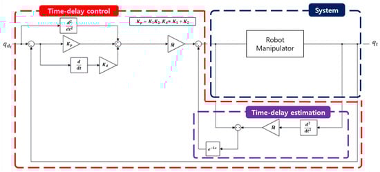
Figure 1.
Diagram of the system controlled with a TDC input (5).
In Ref. [], it is shown that the TDE error is bounded by a positive value such that
Here, if the TDE error, , equals zero, the tracking error also converges to zero since and are positive-definite matrices. The TDE error is commonly assumed to be zero when the sampling period L is sufficiently small. However, the sampling period cannot practically be considered zero due to the limitations that exist in digital controllers. Therefore, ASMC schemes are used simultaneously alongside TDC to compensate for the TDE error, .
In ASMC schemes, a conventional sliding variable [] can be defined as follows:
Using this sliding variable (8), the ASMC input torque combined with that of the TDC scheme can be derived as follows:
where is the adaptive gain matrix, which is designed as a positive-definite diagonal matrix, and .
As shown in the literature [,], the adaptive gain matrix that can suppress overall TDE errors can guarantee that the sliding variable (8) lies on the sliding surface. In the inequality (7), however, an excessively large ASMC gain in a vicinity of the sliding surface can enhance chattering phenomenon due to the sampling interval. Although many studies have aimed at improving adaptive gain matrix , there still exists room for improvement due to trade-offs between improved tracking performance and reduced chattering. Therefore, to tackle this issue, this paper proposes a novel ASMC method using a novel adaptive law based on a novel sliding variable.
3. Proposed ASMC for Robot Manipulators
As shown in Figure 2, this section proposes an ASMC scheme that uses a novel adaptive law based on a quasi-convex function and an average sliding variable. To derive the proposed ASMC input, the average sliding variable is defined as follows:
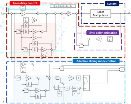
Figure 2.
Diagram of the system controlled with the proposed ASMC (12).
Based on the sliding variable (10), the proposed ASMC for the robot manipulator (4) can be represented as follows.
Here, the proposed control gain in the gain matrix is determined by the following adaptive law:
where is a positive constant; , are positive gains; is an initial time; and is a quasi-convex function defined as
The proposed ASMC method is constructed with the novel sliding variable (10) and the adaptive law (13). Therefore, highlighted areas in Figure 2 represent the differences compared to the conventional ASMC input (9).
The trajectory of the quasi-convex function (14), which simultaneously contains convex and concave parts, is shown in Figure 3. According to Lemma 1, since the second derivative of the quasi-convex function (14) can be calculated as follows:
the quasi-convex function (14) is concave when and convex when . When the adaptive law only uses convex functions as shown in Figure 3, there is a steep slope in the vicinity of the sliding surface and zero slope at the origin. If concave functions are used instead, there is a steep slope at the origin, and the slope is close to zero in the vicinity of the sliding surface. In contrast to these functions, the quasi-convex function (14) has slopes close to zero at both the origin and in the vicinity of the sliding surface, which results in gradual changes to the ASMC gain at the gain switching point satisfying and at the phase switching point, which is the origin.
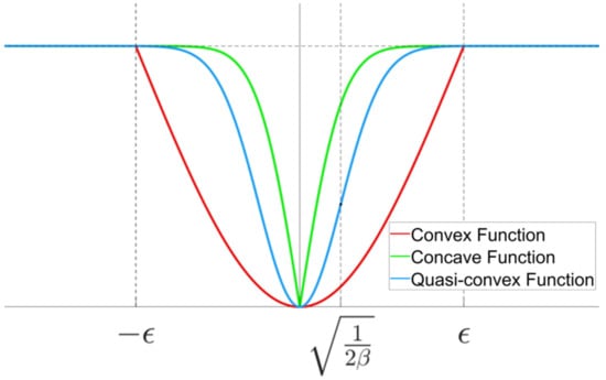
Figure 3.
Trajectory of the quasi-convex function (14).
Remark 1.
Compared to the conventional sliding variable (8), the proposed one also makes use of delayed angle tracking errors and their time derivatives. In addition, a quasi-convex function-based adaptive law is proposed for the ASMC scheme. To the best of the authors’ knowledge, a quasi-convex function has not been used in an ASMC scheme. Since quasi-convex functions can contain both convex and concave parts, the proposed adaptive laws use a quasi-convex function that is convex at the origin and concave at the gain switching point. The effectiveness of the proposed approach is demonstrated through improved tracking performance.
Theorem 1.
Given positive-definite diagonal matrices , , positive scalars , , and a sampling period L, the sliding variable of the robot manipulator (2) controlled by the proposed ASMC (12) using the adaptive gain (13) enters the vicinity of the sliding surface, . Then, the sliding variable is guaranteed to be UUB with the following bound:
where is the maximum value of .
Proof.
The proof is given in Appendix A. □
Remark 2.
Theorem 1 successfully shows the stability of the sliding variable in terms of UUB stability. Since the parameter ϵ, which determines the width of the vicinity of the sliding surface, is a predefined value, the tracking error performance can be chosen according to the choice of ϵ.
4. Simulation
4.1. Simulation Setup
For the simulation, we consider the 2-DOF robot manipulator (2) with the following matrices obtained from [].
where is the angle of the joint i. The length of the links are set as , . The loads of the end tips are set as , . The friction coefficients are , , and . The gravitational acceleration is , and the desired angles are given by , , , and . The adjustable gains in the input torque (12) are set as , , and . We design the parameters of the adaptive law in (13) as follows: , , and .
4.2. Simulation Results
The effectiveness of the proposed ASMC is validated through simulations, which compare the proposed approach with the existing ASMC method in []. For fair comparisons, the gain matrix is obtained from []. Figure 4 shows the tracking errors between the proposed ASMC and the ASMC from []. The results show that the proposed ASMC significantly reduces the tracking error compared to that of []. In Figure 5, the dotted line represents the range of . Looking at these figures, we can clearly see that the proposed control input forces the sliding variable to stay in the region . Also, Figure 6 shows that the control input torque of the proposed ASMC is similar to that of [].
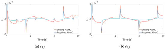
Figure 4.
Tracking error trajectories for each joint in the simulation, existing ASMC [] and proposed ASMC (12).
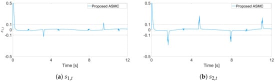
Figure 5.
Sliding variable trajectories for each joint in the simulation, proposed ASMC (12).
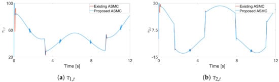
Figure 6.
Input torque trajectories for each joint in the simulation, existing ASMC [] and proposed ASMC (12).
5. Experiment
This section presents the experimental results from implementing the proposed ASMC on a 7-DOF robot manipulator called Franka Research 3, shown in Figure 7. It consists of two parts: a manipulator part and a control box.
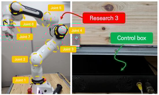
Figure 7.
A 7-DOF robot manipulator (Franka Research 3) and its control box.
5.1. Experimental Setup
In this experiment, we only controlled 4 joints using an Ubuntu 20.04 environment. Franka Research 3 had the following parameters: a mass of 17.8 kg, a maximum payload of 3 kg, and a sampling rate of 1 kHz. The desired angles were , , , , and . The adjustable gains in the input torque (12) were set as , , and . The designed parameters of the adaptive law (13) were set as , , and .
5.2. Experimental Results
Using a real robot manipulator, we compare the proposed ASMC scheme with that of [] in terms of tracking performance and control input torques. In Figure 8, the proposed ASMC has a smaller tracking error than that of []. Figure 9 shows that the input torque of the proposed ASMC is similar to that of []. Although the input torque and chattering characteristics of both algorithms are similar, Figure 8 clearly shows the better tracking performance of the proposed algorithm. Also, Figure 10 clearly shows that the sliding variables recursively converge to the region .
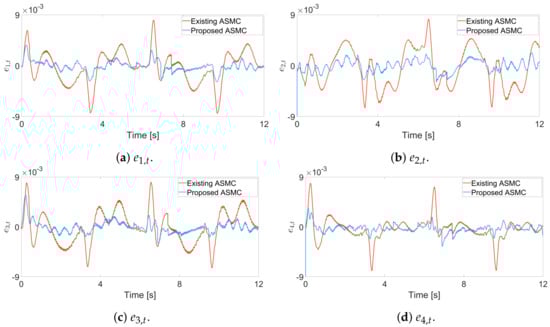
Figure 8.
Tracking error trajectories for each joint in the experiment, existing ASMC [] and proposed ASMC (12).
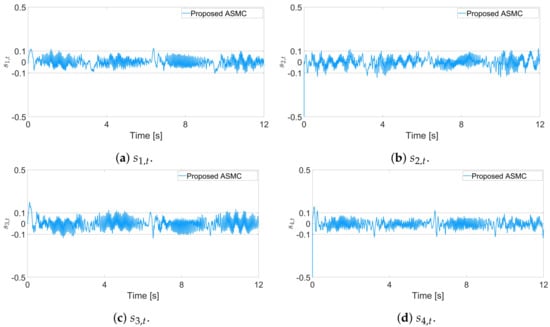
Figure 9.
Sliding variable trajectories for each joint in the experiment, proposed ASMC (12).
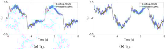
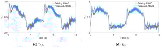
Figure 10.
Input torque trajectories for each joint in the experiment, existing ASMC [] and proposed ASMC (12).
Remark 3.
This paper shows the effectiveness of the proposed methods not only through a simulation but also through an experiment conducted using a real robot manipulator called Franka Research 3. Therefore, the proposed ASMC is a highly practical method that can be applied to various manipulator systems.
6. Conclusions
This paper proposes a novel adaptive law that uses a quasi-convex function and an average sliding variable within an ASMC scheme. To improve tracking performance while maintaining or even reducing chattering, the proposed adaptive law is based on a quasi-convex function that is convex at the origin and concave at the gain switching point. This paper also proves that the proposed sliding variable of robot manipulators controlled by the proposed ASMC is UUB. The simulation and experimental results demonstrate the effectiveness of the proposed methods in terms of improved tracking performance. In a future work, optimization problems related to ASMC parameters including , , , and to control 8- or 9-DOF robot manipulators will be discussed.
Author Contributions
Conceptualization, J.W.L., H.M.A. and S.Y.L.; Funding acquisition, S.Y.L.; Investigation, D.H.S.; Methodology, S.Y.L.; Project administration, S.Y.L.; Software, D.H.S. and J.W.L.; Validation, H.M.A.; Visualization, D.H.S.; Writing—original draft, D.H.S. and S.Y.L.; Writing—review and editing, D.H.S. and S.Y.L. All authors have read and agreed to the published version of the manuscript.
Funding
This work was supported by the Soonchunhyang University Research Fund. This research was supported by “Regional Innovation Strategy (RIS)” through the National Research Foundation of Korea (NRF) funded by the Ministry of Education (MOE) (2021RIS-004).
Data Availability Statement
Data is contained within the article.
Conflicts of Interest
The authors declare no conflicts of interest.
Appendix A
Proof of Theorem 1.
To prove Theorem 1, Let us define the Lyapunov function as follows:
Based on the definitions (10) and (11), the time derivative of the Lyapunov function can be computed as follows:
Since the proposed adaptive law (13) consists of two regions: and , the negative condition of is guaranteed for as follows:
where is the minimum eigenvalue of the matrix . Therefore, the region can be reached if the adaptive control gain increases. In the region , however, the negative condition of cannot be directly guaranteed as follows:
Even if the sliding variable leaves the region , becomes negative again due to condition (A3) and, thus, the sliding variable repeatedly converges to . According to the Lyapunov theorem and inequality (A3), the convergence time of the sliding variable to the region is finite. Therefore, there exists an upper bound of the control gain , and thus a maximum value for also exists. Since the Lyapunov function (A1) has the following lower and upper bounds:
in the region , the following upper bound of can be obtained:
References
- Guo, W.; Zhu, Y.; He, X. A Robotic Grinding Motion Planning Methodology for a Novel Automatic Seam Bead Grinding Robot Manipulator. IEEE Access 2020, 8, 75288–75302. [Google Scholar] [CrossRef]
- Mitchell, B.; Koo, J.; Iordachita, I.; Kazanzides, P.; Kapoor, A.; Handa, J.; Hager, G.; Taylor, R. Development and application of a new steady-hand manipulator for retinal surgery. In Proceedings of the 2007 IEEE International Conference on Robotics and Automation, Roma, Italy, 10–14 April 2007; pp. 623–629. [Google Scholar]
- Weinrib, H.P.; Cook, J.Q. Rotational technique and microsurgery. Microsurgery 1984, 5, 207–212. [Google Scholar] [CrossRef]
- Baek, J.; Jin, M.; Han, S. A new adaptive sliding-mode control scheme for application to robot manipulators. IEEE Trans. Ind. Electron. 2016, 63, 3628–3637. [Google Scholar] [CrossRef]
- Zhu, Y.; Liu, Z.; Jiang, B.; Zhu, Q. Adaptive fixed-time fuzzy fault-tolerant control for robotic manipulator with unknown friction and composite actuator faults. J. Frankl. Inst. 2024, 361, 107025. [Google Scholar] [CrossRef]
- Ma, R.; Chen, J.; Lv, C.; Yang, Z.; Hu, X. Backstepping Control with a Fractional-Order Command Filter and Disturbance Observer for Unmanned Surface Vehicles. Fractal Fract. 2023, 8, 23. [Google Scholar] [CrossRef]
- Abe, A. Trajectory planning for flexible Cartesian robot manipulator by using artificial neural network: Numerical simulation and experimental verification. Robotica 2011, 29, 797–804. [Google Scholar] [CrossRef]
- Li, T.; Zhang, G.; Zhang, T.; Pan, J. Adaptive Neural Network Tracking Control of Robotic Manipulators Based on Disturbance Observer. Processes 2024, 12, 499. [Google Scholar] [CrossRef]
- Kern, J.; Marrero, D.; Urrea, C. Fuzzy Control Strategies Development for a 3-DoF Robotic Manipulator in Trajectory Tracking. Processes 2023, 11, 3267. [Google Scholar] [CrossRef]
- Jin, M.; Kang, S.H.; Chang, P.H.; Lee, J. Robust control of robot manipulators using inclusive and enhanced time delay control. IEEE/ASME Trans. Mechatronics 2017, 22, 2141–2152. [Google Scholar] [CrossRef]
- Wang, X.; Zhang, R.; Li, G.; Wang, Q.; Wen, Y. Time Delay Estimation Control of Permanent Magnet Spherical Actuator Based on Gradient Compensation. Electronics 2021, 11, 66. [Google Scholar] [CrossRef]
- Islam, S.; Liu, X.P. Robust sliding mode control for robot manipulators. IEEE Trans. Ind. Electron. 2010, 58, 2444–2453. [Google Scholar] [CrossRef]
- Bandyopadhyay, B.; Janardhanan, S.; Spurgeon, S.K. Advances in Sliding Mode Control; Lecture Notes in Control and Information Sciences; Springer: Berlin/Heidelberg, Germany, 2013; Volume 440. [Google Scholar]
- Han, S.I.; Lee, J. Finite-time sliding surface constrained control for a robot manipulator with an unknown deadzone and disturbance. ISA Trans. 2016, 65, 307–318. [Google Scholar] [CrossRef] [PubMed]
- Park, J.; Kwon, W.; Park, P. An improved adaptive sliding mode control based on time-delay control for robot manipulators. IEEE Trans. Ind. Electron. 2022, 70, 10363–10373. [Google Scholar] [CrossRef]
- Lv, Z.; Jin, S.; Xiong, X.; Yu, J. A New Quick-Response Sliding Mode Tracking Differentiator with its Chattering-Free Discrete-Time Implementation. IEEE Access 2019, 7, 130236–130245. [Google Scholar] [CrossRef]
- Huang, Y.J.; Kuo, T.C.; Chang, S.H. Adaptive sliding-mode control for nonlinear systems with uncertain parameters. IEEE Trans. Syst. Man Cybern. Part B (Cybern.) 2008, 38, 534–539. [Google Scholar] [CrossRef]
- Utkin, V.I. Adaptive Sliding Mode Control; Springer: Berlin/Heidelberg, Germany, 2013; pp. 21–53. [Google Scholar]
- Plestan, F.; Shtessel, Y.; Bregeault, V.; Poznyak, A. New methodologies for adaptive sliding mode control. Int. J. Control 2010, 83, 1907–1919. [Google Scholar] [CrossRef]
- Hsu, L.; Oliveira, T.R.; Cunha, J.P.V.; Yan, L. Adaptive unit vector control of multivariable systems using monitoring functions. Int. J. Robust Nonlinear Control 2019, 29, 583–600. [Google Scholar] [CrossRef]
- Roy, S.; Roy, S.B.; Lee, J.; Baldi, S. Overcoming the underestimation and overestimation problems in adaptive sliding mode control. IEEE/ASME Trans. Mechatronics 2019, 24, 2031–2039. [Google Scholar] [CrossRef]
- Obeid, H.; Fridman, L.M.; Laghrouche, S.; Harmouche, M. Barrier function-based adaptive sliding mode control. Automatica 2018, 93, 540–544. [Google Scholar] [CrossRef]
- Shao, K.; Zheng, J.; Wang, H.; Wang, X.; Lu, R.; Man, Z. Tracking control of a linear motor positioner based on barrier function adaptive sliding mode. IEEE Trans. Ind. Inform. 2021, 17, 7479–7488. [Google Scholar] [CrossRef]
- Dempe, S.; Gadhi, N.; Hamdaoui, K. Minimizing the difference of two quasiconvex functions. Optim. Lett. 2020, 14, 1765–1779. [Google Scholar] [CrossRef]
- Hassan, K.K. Nonlinear Systems; Prentice Hall: East Lansing, MI, USA, 2002. [Google Scholar]
- Tyrrell Rockafellar, R. Convex analysis. In Princeton Mathematical Series; Princeton University Press: Princeton, NJ, USA, 1970; Volume 28. [Google Scholar]
Disclaimer/Publisher’s Note: The statements, opinions and data contained in all publications are solely those of the individual author(s) and contributor(s) and not of MDPI and/or the editor(s). MDPI and/or the editor(s) disclaim responsibility for any injury to people or property resulting from any ideas, methods, instructions or products referred to in the content. |
© 2024 by the authors. Licensee MDPI, Basel, Switzerland. This article is an open access article distributed under the terms and conditions of the Creative Commons Attribution (CC BY) license (https://creativecommons.org/licenses/by/4.0/).