Multi-Scale Spatial–Spectral Residual Attention Network for Hyperspectral Image Classification

Abstract

Hyperspectral images (HSIs) encapsulate a vast amount of information due to their expansive size and high number of channel dimensions. However, they are insufficiently utilized for ineffective feature extraction, particularly for regions with few samples and predominant edges. To fully leverage the spatial–spectral features of HSIs, a dual-branch multi-scale spatial–spectral residual attention network (MSRAN) that integrates multi-scale feature extraction with residual attention mechanisms is proposed. MSRAN independently extracts spatial and spectral features through dual branches, minimizing the interference between these features and enhancing the focus on feature extraction in different dimensions. Specifically, in the spectral feature extraction branch, diverse-scale 3D convolution kernels capture extended spectral sequence characteristics and neighborhood spectral features. The convolution fusion emphasizes the weight of the central pixel to be classified, followed by the use of spectral residual attention mechanisms to extract enhanced central-pixel spectral features. In the spatial feature extraction branch, multi-level receptive fields are utilized to extract various fine-grained spatial contours, edges, and local detailed features, which are further processed through spatial residual attention to effectively extract spatial composite features. Finally, the convolution fusion module adaptively integrates the center-enhanced spectral features with multi-level fine-grained spatial features for classification. Extensive comparative experiments and ablation studies demonstrate that MSRAN achieves highly competitive results on two classic datasets from Pavia University and Salinas as well as on a novel dataset of WHU-Hi-LongKou.

1. Introduction

Remote sensing images with high resolution and rich spectral information play a pivotal role in diverse fields, such as plant pest and disease detection [1,2,3], mineral exploration [4,5], crop yield estimation [6,7], and environmental monitoring [8,9]. Fang et al. [10] estimated the soil moisture using satellite remote sensing data by integrating Bayesian depth image prior (BDIP) downsampling with a deep fully convolutional neural network. Pang et al. [11] developed an advanced platform combining Lidar, CCD cameras, and hyperspectral sensors for detailed forest monitoring and analysis. Guo et al. [12] utilized vegetation indices (VIs) and texture features (TFs) from unmanned aerial vehicle (UAV) hyperspectral images to create a disease monitoring model based on the partial least squares regression (PLSR) for detecting wheat yellow rust. Hyperspectral images (HSIs) [13], composed of hundreds of spectral bands, offer finer spectral divisions than other images, which provides powerful material discrimination capabilities. As a critical technology in these applications, HSI classification employs traditional methods like the support vector machine (SVM) [14], decision tree (DT) [15], and maximum likelihood classifier (MLC) [16]. However, these conventional methods primarily extract shallow features and often overlook deeper characteristics with the manual setting of feature selectors significantly impacting the classification accuracy.

In contrast to traditional HSI classification techniques, deep learning methods have the advantages of automatic feature learning and superior classification capabilities. They have achieved significant progress in various domains. Consequently, an increasing number of scholars are exploring HSI classification through deep learning approaches. Boulch et al. [17] proposed an autoencoder (AE)-based network to perform HSI classification by combining multi-layer AE and pooling layers. Chen et al. [18] proposed a Deep Belief Network (DBN)-based method to extract both shallow and deep features from HSI images for classification. The advent of Convolutional Neural Networks (CNNs) significantly enhanced the image classification accuracy. Given the abundance of sequential information in the spectral channels of HSIs, Mou et al. [19] applied recurrent neural networks to HSI classification for the first time and achieved commendable results. Hu et al. [20] effectively extracted spectral features from HSIs using a stack of five 1D-CNNs. Sharma et al. [21] utilized 2D-CNNs to extract contextual spatial feature information from dimensionality-reduced HSIs, improving the classification performance with limited HSI training samples. However, utilizing the information from spectral or spatial features alone cannot fully take advantage of the rich features of HSIs. The fusion of spectral and spatial features is a beneficial complement to HSI classification. Yang et al. [22] combined the features of 1D-CNN and 2D-CNN frameworks to extract spatial and spectral features, respectively, and then fused these features through a fully connected layer for classification. Joint spatial–spectral features can significantly improve the HSI classification accuracy. Nevertheless, dual-branch networks that extract features from spectral and spatial dimensions separately can lead to the loss of some original information, resulting in inadequate spatial–spectral joint features. The introduction of three-dimensional Convolutional Neural Networks has effectively mitigated this issue. Li et al. [23] proposed an end-to-end five-layer 3D-CNN network. Chen et al. [24] combined the 3D-CNN with regularization techniques to effectively extract original three-dimensional features and reduce overfitting in neural networks. Zhong et al. [25] introduced an end-to-end Spectral–Spatial Residual Network for HSI classification, which takes the original three-dimensional data cube as the input and extracts both spectral and spatial features using the 3D-CNN. Qi et al. [26] combined multi-scale and residual concepts to extract deeper features from different receptive fields and classify HSIs. Li et al. [27] integrated attention mechanisms into the Dual-Branch Multi-Attention Network to refine hyperspectral features and achieve a better classification performance. Meng et al. [28] proposed a new deep residual involution network (DRIN) for HSI classification. By using an enlarged involution kernel, the long-distance spatial interactions can be well-modeled.

Although CNNs have shown good performance in the field of HSI classification, there are still challenges to be addressed. For example, labeled HSIs require substantial human and material resources, so maximizing the utilization of existing data when HSI samples are limited is crucial. Furthermore, distinguishing the varying contributions of deep features to each node of the neural network is a challenging task. Lastly, the extraction of joint spatial–spectral features can lead to interference, and determining the correct combination of extracted features in multi-branch networks poses a challenge.

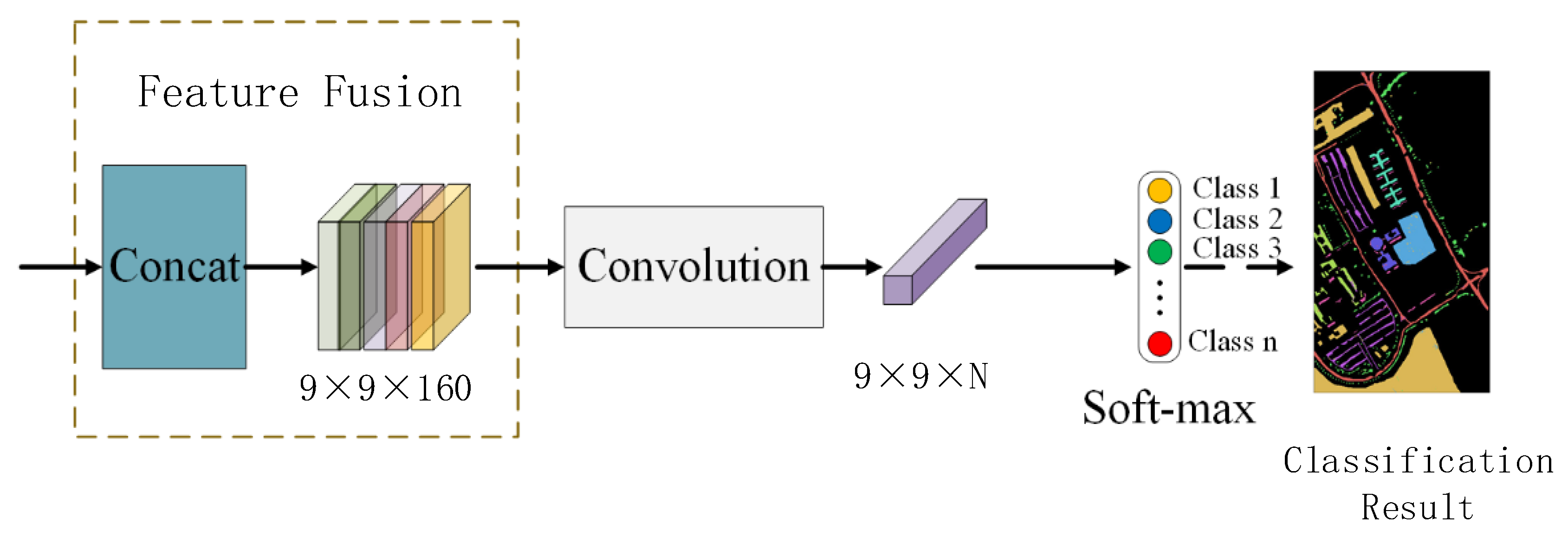
To mitigate these issues, a novel model combining 3D-CNN, 2D-CNN, multi-scale mechanisms [29,30], and residual attention mechanisms [31,32], namely MSRAN, is proposed. This method independently extracts spatial and spectral features through dual branches to minimize the interference between features of different dimensions. It then uses multi-scale mechanisms to enrich the feature diversity and employs spatial residual attention and spectral residual attention to identify effective features, thereby improving feature utilization. Finally, convolutional adaptive fusion integrates spatial texture features and spectral sequence features for classification. The contributions of this paper can be summarized as follows.

• We present a Dual-Branch Multi-Scale Residual Spatial–Spectral Attention Network to classify the hyperspectral remote sensing images. This network independently extracts spatial and spectral features, minimizes the interference between these two types of information, and enables the model to focus on multi-dimensional features.
• We extract the sequential and neighboring spectral features using different-sized convolution kernels. Meanwhile, multi-scale 2D convolution is employed to capture spatial features by superimposing various receptive fields. This approach improves the ability to classify the multi-boundary samples by highlighting the central pixel weight and capturing the ground contours and local details.
• The proposed MSRAN method employs dual residual spectral and spatial attention mechanisms to identify the important features for hyperspectral image classification, which eliminates the disruptive features and enhances the utilization of spatial and spectral features.
• A comprehensive assessment of the proposed MSRAN method is conducted through extensive ablation studies and comparative experiments on three datasets from Pavia University (PU) [33], Salinas Valley (SV) [33], and WHU-Hi-LongKou (WHKL) [34]. The results demonstrate a great improvement in the classification accuracy over advanced methods.

The subsequent parts of this paper are organized as follows: Section 2 discusses the proposed MSRAN method. In Section 3, ablation studies and comparative experiments are conducted to verify the effectiveness and competitiveness of the proposed model. Section 4 summarizes our work.

2. Proposed MSRAN for HSI Classification

2.1. Structure of the Multi-Scale Spatial–Spectral Residual Attention Network

In HSI classification methods, spatial and spectral features are directly extracted and fused to improve the accuracy, potentially leading to interactions between the two branches [35]. Although some improved approaches extract spectral and spatial features in parallel, further optimization of these features is necessary. To enhance the HSI classification performance, this paper extracts joint spatial–spectral, spatial texture, and spectral sequence features from HSIs at different receptive fields using the multi-scale 3D-CNN and 2D-CNN, followed by residual attention optimization. The structure of the proposed MSRAN method is illustrated in Figure 1. Initially, the original HSI is cropped into overlapping blocks to reduce the input data volume. These cropped HSI blocks are then fed into two branches for spectral and spatial feature extraction, respectively, followed by feature fusion classification. Specifically, in the spectral branch, various-scale 3D convolutions are utilized to extract joint spatial–spectral and spectral sequence features. To enhance the spectral distinguishability of different materials, an improved residual spectral attention block reallocates the weights of features, thus augmenting the salient spectral characteristics while filtering out noise and less relevant features. In the spatial feature extraction branch, a combination of multi-scale 2D-CNNs extracts spatial texture features from different receptive fields. For instance, small convolution kernels focus on spatial texture features, while larger ones are more adept at capturing object contour characteristics. However, due to parameter issues associated with large convolution kernels, we expand the receptive field by stacking sequential 2D-CNNs, thus attaining more spatial context features while reducing the number of parameters. Subsequently, to improve the spatial distinguishability of different materials, residual spatial attention reallocates the contributions of different depth features to the neural network nodes, enhancing significant spatial characteristics and diminishing the weights of irrelevant spatial features to the target task. Finally, the convolution fusion module combines the spectral and spatial optimized features through the attention mechanism and uses the Softmax function to classify the fused spatial spectral features.

2.2. Spectral Feature Extraction Branch

In the spectral feature extraction branch, the multi-scale 3D-CNN is used to design the spectral feature extraction module, as shown in Figure 2. The joint spatial–spectral cubic features are extracted by using a three-dimensional convolution with a convolution kernel of $3\times 3\times 3$, and the spectral sequence features are extracted by using a three-dimensional convolution with a convolution kernel of $5\times 1\times 1$. Subsequently, the spatial–spectral features and spectral features are summed and then fused through convolution. Specifically, the input HSI is denoted as $x\in {ℝ}^{c\times w\times h}$, where $c$ represents the spectral dimension, and $w$ and $h$ respectively indicate the width and height of the input HSI. The spectral features extracted by convolution at different scales are activated by Relu and summed to obtain the output feature $y$. The calculation formulas are shown in Equations (1)–(3):

$$x_i=\mathrm{Relu}\left(Con{v}_{3\times 3\times 3}\left(x\right)\right),i=1$$

(1)

$$x_i=\mathrm{Relu}\left(Con{v}_{5\times 1\times 1}\left(x\right)\right),i=2$$

(2)

$$y=x_1+x_2$$

(3)

In the spectral feature extraction module, $x_i\in {ℝ}^{c\times w\times h}\left(i=1,2\right)$ represents the Relu-activated convolutional features at different spectral scales, where i denotes the serial number of convolutions. The convolution operations in $Con{v}_{3\times 3\times 3}\left(·\right)$ and $Con{v}_{5\times 1\times 1}\left(·\right)$ are similar. Taking the latter as an example, it is a 3D convolution with a kernel size of $5\times 1\times 1$, where the spectral dimension is 5, and the spatial dimensions are $1\times 1$.

To refine the spectral features and redistribute the feature contributions to nodes, we introduce the spectral residual attention module by using the residual structure, as shown in Figure 3. This module employs maximum pooling and average pooling on the feature matrix to respectively capture decisive features within the target neighborhood and smooth shared neighborhood features. Subsequently, these features are processed through a Multi-Layer Perceptron (MLP) for shared weighting, thereby increasing the weights that are favorable for target feature classification. The module then utilizes a dual residual structure to mitigate network degradation issues and expedite network updates. Specifically, the extracted spectral features y undergo convolution with a $B\times 1\times 1$ kernel, mapping the information from the spectral dimension to the channel dimension, resulting in the output spectral feature $\widehat{y}$. This feature is then fed into the spectral channel attention module for further processing. The spectral feature $\widehat{y}\in {ℝ}^{c\times w\times h}$ undergoes maximum pooling and average pooling, followed by a parameter-shared MLP to obtain preassigned weights. The MLP consists of two layers. The first layer produces a feature map of size $\frac{c}{r}\times 1\times 1$ (where $r$ is the feature compression ratio), while the second layer yields a feature map with the dimensions $c\times 1\times 1$. The feature map outputs from the second layer of the MLP are added together, and then an activation function is used to generate the redistributed weights $M_c\in {ℝ}^{c\times 1\times 1}$. These weights are subsequently combined with the spectral feature $\widehat{y}$ to enhance the feature representation. $\widehat{y}$ is added to the output of the spectral feature extraction module $z$. The formulas are shown in Equations (4)–(6):

$$\widehat{y}=\mathrm{Re}lu\left(Con{v}_{B\times 1\times 1}\left(y\right)\right)$$

(4)

$$\begin{array}{cc}\hfill M_C\left(\widehat{y}\right)& = \sigma \left(MLP\left(AvgPool\left(\widehat{y}\right)\right)+MLP\left(MaxPool\left(\widehat{y}\right)\right)\right)\hfill \\ \hfill & = \sigma \left(W_1\left(W_0\left({\widehat{y}}_{avg}^C\right)\right)+W_1\left(W_0\left({\widehat{y}}_{\max }^C\right)\right)\right)\hfill \end{array}$$

(5)

$$z=M_c\left(\widehat{y}\right)\times \widehat{y}+\widehat{y}$$

(6)

where $Con{v}_{B\times 1\times 1}\left(·\right)$ represents a 3D convolution with a kernel size of $B\times 1\times 1$, $B$ is the spectral dimension size of the input $y$, and $AvgPool(·)$ and $MaxPool(·)$ represent the average pooling and maximum pooling operations, respectively. $\sigma$ is the Sigmoid activation function, and $M_c\left(·\right)$ denotes the weights generated by the MLP. After simplification in Equation (5), $W_0$ and $W_1$ are the weights of the first and second layers of MLP, while ${\widehat{y}}_{avg}^C$ and ${\widehat{y}}_{\max }^C$ represent the feature matrices after average pooling and maximum pooling.

2.3. Spatial Feature Extraction Branch

The spatial dimension of the HSI is significantly smaller than the spectral dimension, which can easily lead to the Hughes phenomenon [36] in the HSI classification. To minimize the disparity between the spectral and spatial dimensions, spectral dimension compression is performed while extracting features using the 2D-CNN. This not only reduces the loss of spectral information but also decreases the number of model parameters. As shown in Figure 4, in order to fully extract and utilize the spatial neighborhood features, this paper attempts to combine different receptive fields and the multi-level 2D-CNN to extract the features of four branches and then performs spatial attention to screen the effective features to obtain the output of each branch. Specifically, the first branch uses a single 2DConv with a convolution kernel size of $3\times 3$ to extract the spatial details and texture features under a small-scale receptive field. The second branch employs a 2DConv with a convolution kernel size of $5\times 5$ to extract spatial object contour features under a larger receptive field. The third branch initially utilizes a 2DConv with a convolution kernel size of $5\times 5$ for a large-scale receptive field, followed by a 2DConv with a convolution kernel size of $3\times 3$ to further expand the receptive field and extract environmental features surrounding spatial objects. In branch four, average pooling is used to obtain smooth neighborhood features to assist with the fusion of various levels of spatial features. Each branch is numbered $M_i\left(i=1,2,3,4\right)$, where $i$ represents the number of different branches. The calculation formula is shown in Equation (7):

$$K_i=\left\{\begin{array}{c}\mathrm{Relu}\left(Conv2d_{3\times 3}\left(\widehat{x}\right)\right),i=1\\ M_s\left(\mathrm{Relu}\left(Conv2d_{5\times 5}\left(\widehat{x}\right)\right)\right),i=2\\ M_s\left(\mathrm{Relu}\left(Conv2d_{5\times 5}\left(Conv2d_{3\times 3}(\widehat{x})\right)\right)\right),i=3\\ AvgPooling\left(\widehat{x}\right),i=4\end{array}\right.$$

(7)

where $Conv2d_{3\times 3}\left(·\right)$ represents a 2D convolution with a size of $3\times 3$, $\mathrm{Relu}\left(·\right)$ is the Relu activation function, ${\mathrm{M}}_S\left(·\right)$ denotes the spatial residual attention, $AvgPooling\left(·\right)$ signifies average pooling, and $\sigma$ is the Sigmoid activation function.

Based on the extracted spatial features in two dimensions, within the spatial residual attention, as illustrated in Figure 5, decisive features within the target neighborhood and smoothed neighborhood features are obtained through maximum pooling and average pooling. After concatenating these features, convolution is used for feature discrimination, focusing on characteristics that are beneficial for target classification. Finally, a dual-path residual is employed to accelerate network training and prevent network degradation. Specifically, the spatial feature $\widehat{x}\in {ℝ}^{8\times w\times h}$ is compressed through maximum and average pooling along the spectral dimension. Then, the redistributed weights $M_s\in {ℝ}^{8\times w\times h}$ are generated through convolution mapping and the Sigmoid activation function and are multiplied with the spatial feature $\widehat{x}$. Finally, the result of this multiplication is directly added to $\widehat{x}$, yielding the output $K$ of the spatial feature extraction module.

2.4. Feature Fusion and Classification Module

The spectral and spatial features optimized by the attention mechanism are fused through a cascading operation, as shown in Figure 6. The features are then mapped through convolution to output $N$ dimensions, where $N$ is the number of classes of ground objects in the training samples. Finally, the classification result is obtained through a Softmax operation, as calculated in Equation (8):

$$S=\delta \left(Con{v}_{1\times 1}\left(\left[Z,K_i\right]\right)\right),i=1,2,3,4$$

(8)

where $\delta$ Softmax represents the Softmax function, and $i$ is the number of different branches in the spatial feature extraction module. In the spatial–spectral feature fusion module, the spectral and spatial features are fused through a cascading operation. This is followed by a convolution operation to obtain spatial–spectral joint features with consistent dimensions, which are then further integrated through feature fusion.

3. Experimental Results and Analysis

To validate the effectiveness of the proposed MSRAN classification method, a series of ablation and comparative experiments were conducted using two classic datasets, the PU dataset and the SV dataset, along with a novel dataset, the WHLK dataset. The contributions of different modules to the network and the classification performance of various algorithms were assessed using multiple indicators (Overall Accuracy—OA, Average Accuracy—AA, the Kappa $\times 100$ (K) coefficient [37], and the category-wise classification accuracy for each dataset).

3.1. Experimental Datasets

3.1.1. Pavia University Dataset

This dataset was captured by the Reflection Optical System Imaging Spectroradiometer (ROSIS) in the university town of Pavia in northern Italy in 2001. It consists of 115 spectral bands. Twelve spectral bands were removed due to noise, leaving 103 spectral bands for the experimental study. The image size is 610 × 340 pixels, the spectral resolution is 4 nm, and the spatial resolution is 1.3 m/pixel. This dataset includes real-life scenarios consisting of nine different types of land cover, with 42,776 labeled samples. In this study, 5% of the samples were used as the training set and validation set, and the rest were used as the test set. Figure 7 shows the pseudo-color image and ground truth map.

Table 1. Categories and corresponding training, validation, and test sample numbers for the PU dataset.

NO.	Category	Sample Size	Train/Val	Test
1	Asphalt	6631	332	5967
2	Meadows	18,649	932	16,785
3	Gravel	2099	105	1889
4	Trees	3064	153	2758
5	Painted metal sheets	1345	67	1211
6	Bare soil	5029	251	4527
7	Bitumen	1330	67	1196
8	Self-blocking bricks	3682	184	3314
9	Shadows	947	47	853
Total		42,776	2138	38,500

lists the numbers of training, validation, and testing samples for each category.

3.1.2. Salinas Valley Dataset

This dataset was captured by the Airborne Visible/Infrared Imaging Spectroradiometer (AVIRIS) sensor in the Salinas Valley agricultural region of California in 1998. It originally contained 224 spectral bands, of which 204 were retained for experimental studies after removing 20 water absorption bands. The image size is 512 × 217 pixels, the wavelength range is 400–2500 nm, and the spatial resolution is 3.7 m/pixel. This dataset contains 16 different types of land cover, with 54,129 labeled samples. In this study, 5% of the samples were used as the training set and validation set, and the rest were used as the test set. Figure 8 shows the pseudo-color image and ground truth map.

Table 2. Categories and corresponding training, validation, and test sample numbers for the SV dataset.

NO.	Category	Sample Size	Train/Val	Test
1	Broccoli Gl	2009	100	1809
2	Broccoli G2	3726	186	3354
3	Fallow	1976	99	1778
4	Fallow R	1394	70	1254
5	Fallow_S	2678	134	2410
6	Stubble	3959	198	3563
7	Celery	3579	179	3221
8	GrapesU	11,271	564	10,143
9	Soil_V	6203	310	5583
10	Comn_S	3278	164	2950
11	Lettuce R4	1068	53	962
12	Lettuce R5	1927	96	1735
13	Lettuce R6	916	46	824
14	Lettuce R7	1070	54	962
15	Vineyard U	7268	363	6542
16	Vineyard V	1807	90	1627
Total		54,129	2706	48,717

lists the numbers of training, validation, and testing samples for each category.

3.1.3. WHU-Hi-LongKou Dataset

This dataset was captured by the Headwall Nano-Hyperspec imaging sensor from 13:49 to 14:37 on 17 July 2018 over Longkou Town, Hubei Province, China. It consists of 270 spectral bands that are used for experimental studies. The image is 550 × 400 pixels, the wavelength range is 400–1000 nm, and the spatial resolution is 0.463 m/pixel. This dataset contains nine land cover types with 204,542 pixels labeled. In this study, 1% of the samples were used as the training set and validation set, and the rest were used as the test set. Figure 9 shows the pseudo-color image and ground truth map.

Table 3. Categories and corresponding training, validation, and test sample numbers for the WHLK dataset.

NO.	Category	Sample Size	Train/Val	Test
1	Corn	34,511	345	33,821
2	Cotton	8374	84	8206
3	Sesame	3031	30	2971
4	Broad-leaf soybean	63,212	632	61,948
5	Narrow-leaf soybean	4151	42	4067
6	Rice	11,854	119	11,616
7	Water	67,056	671	65,714
8	Roads and houses	7124	71	6982
9	Mixed weed	5229	52	5125
Total		204,542	2046	200,450

lists the numbers of training, validation, and testing samples for each category.

3.2. Experimental Settings

In the experiments, the Adam optimizer was utilized, with the default setting of 64 samples per batch for training. The learning rate was set to 1 × 10⁻³ by default, and the patch size was set to nine by default. For training periods, the PU and SV datasets were subjected to 300 epochs, while the WHLK dataset was set to 200 epochs. The parameter settings for other comparative methods were consistent with those reported in the corresponding literature. All training samples underwent the same data preprocessing methods, and the results were derived from the average of multiple experiments. In order to ensure fairness in the experimental process, all HSI classification methods were implemented on the same computing workstation. The workstation was equipped with 40 GB of memory, an Intel 8255C CPU, and an RTX 3080 GPU. The experiments were conducted on the Ubuntu 18.04 platform using the PyTorch 1.8.1 framework.

In order to quantitatively compare the effectiveness of the method presented in this paper with multiple other approaches, four quantitative evaluation metrics were adopted: OA, AA, the K coefficient, and the classification accuracy for individual categories in each dataset. OA represents the percentage of samples correctly classified by the model in the entire dataset, which is used as a measure of the overall performance, where the higher the value, the better the performance. AA is the mean of the precision values for each category, providing a comprehensive assessment of the performance across categories. The Kappa coefficient is a measure of the consistency between the model and random classification, taking into account the randomness in the classification results, thereby offering more reliability than the mere OA. The Kappa coefficient ranges between −1 and 1, where 0 indicates agreement with random classification and 1 denotes complete agreement. The category classification accuracy of each dataset refers to the proportion of correctly classified samples in each category.

3.3. Experimental Results and Analysis

3.3.1. Ablation Studies

To demonstrate the contribution of each module, ablation experiments were performed using a controlled module variable approach. The MSRAN is mainly composed of the multi-scale spectral residual network (spectral branch), the multi-scale spatial residual network (spatial branch), and the feature fusion module. Different combinations of these modules were tested to assess their contributions. Since the feature fusion module integrates feature fusion and classification tasks, it was included by default in our experiments. As shown in

Table 4. Contributions of different components to the proposed MSRAN method.

	Multi-Scale Mechanism	Spectral Branch	Spatial Branch	Metric	PU	SV	WHLK
NET-1	-	√	×	OA%	97.80	93.63	90.95
				AA%	96.87	94.19	72.62
				K%	97.08	92.92	88.52
NET-2	-	×	√	OA%	88.07	89.70	79.18
				AA%	79.88	90.75	45.63
				K%	83.84	88.49	73.39
NET-3	×	-	-	OA%	92.51	88.58	89.23
				AA%	88.98	90.35	61.98
				K%	90.00	87.21	85.68
NET-4	√	√	√	OA%	98.82	97.03	98.86
				AA%	97.37	97.82	95.80
				K%	98.44	96.68	98.50

The bold entities indicate the highest value. ×: does not exist, √: exists, -: not relevant.

, a comparison between NET-1 and NET-4 revealed that the inclusion of multi-scale spatial residual attention in NET-4 led to increases in the OA of 1.02% and 3.40% for the PU and SV datasets, respectively. This improvement is attributed to the fact that HSIs encompass both spatial and spectral information, making the joint spatial–spectral features more suitable for HSI classification tasks. The incorporation of spatial residual attention mechanisms enables the network to focus more on features that are effective for classification. Notably, for the WHLK dataset, the introduction of multi-scale spatial–spectral residual attention mechanisms resulted in a significant 7.91% increase in the OA. This can be attributed to the higher spatial resolution of the WHLK, which provides richer details for land cover spatial features. Multi-scale feature extraction can extract more levels of land cover contours, edges, and local details through different receptive fields, thereby enhancing the precision of the classification features. By comparing it with the NET-2, the introduction of multi-scale spectral residual attention in the NET-4 resulted in notable OA improvements of 10.75%, 7.33%, and 19.68% on three HSI datasets, respectively. This improvement is partly due to the advantages brought by the joint spatial–spectral features and partly because of the use of 3 × 3 × 3 three-dimensional convolution kernels and 5 × 1 × 1 one-dimensional convolution kernels. These kernels not only extract longer one-dimensional spectral features but also accommodate three-dimensional neighboring spectral features. Subsequently, spectral residual attention was applied to enhance the utilization of spectral features. In NET-3, the spatial and spectral multi-scale mechanisms are modified to a single scale. Specifically, in the spectral branch, the multi-scale 3DConv is replaced with a single-scale 3DConv with a 3 × 3 × 3 convolution kernel, while in the spatial branch, the multi-level multi-scale convolution is substituted with a single-scale 2DConv with a 5 × 5 kernel. All other experimental settings are retained, as they are in our final NET-4 model. By comparison, our final NET-4 model incorporates a multi-scale mechanism and improves by 6.31%, 8.54%, and 9.63% in terms of the OA on three distinct datasets, respectively. This demonstrates that the multi-scale mechanism is adept at capturing object features of various sizes. The reason for this mainly lies in the fact that the various volumes of different-sized objects lead to diverse scales of edge contours and local detail information. This diversity necessitates the use of different receptive fields for effective feature extraction. The combination of spectral and spatial multi-scale mechanisms enhances our proposed MSRAN method to achieve a superior classification performance.

3.3.2. Comparative Experiments

To validate the effectiveness of the proposed MSRAN method, comparative experiments were conducted against a range of both classical and contemporary networks, including the SVM [14], 1D-RNN [18], 1D-CNN [20], 2D-CNN [21], 3D-CNN [23], DBDA [27], DRIN [28], and LS²CM [38].

Table 5. Classification results of PU datasets with different methods.

NO.	SVM	1DRNN	1DCNN	2DCNN	3D-CNN	DBDA	DRIN	LS2CM	MSRAN
1	83.73	88.74	81.62	79.05	95.76	98.04	98.53	98.63	97.84
2	88.71	95.76	87.32	71.83	97.11	95.34	97.61	97.69	99.78
3	4.74	67.38	1.12	59.43	91.26	96.10	90.26	94.42	96.38
4	89.99	93.54	78.89	82.67	96.19	96.23	97.78	98.85	99.34
5	99.17	99.83	98.48	97.58	99.29	99.67	99.96	99.96	100.0
6	33.21	87.52	38.89	99.74	97.32	98.38	99.48	99.40	99.30
7	0.00	66.75	0.30	98.35	90.98	99.92	98.56	98.56	92.30
8	75.98	75.20	75.22	94.62	93.95	98.92	95.20	97.28	97.57
9	99.94	99.18	99.41	82.77	96.85	98.51	99.88	99.82	99.82
OA%	79.68	89.67	77.54	69.53	95.14	94.74	96.55	97.01	98.82
AA%	65.98	85.99	63.87	77.75	93.92	96.08	96.51	97.28	97.37
K%	71.62	86.29	68.72	64.07	93.61	93.22	95.47	96.09	98.44

The bold entities indicate the highest value.

,

Table 6. Classification results of SV datasets with different methods.

NO.	SVM	1DRNN	1DCNN	2DCNN	3D-CNN	DBDA	DRIN	LS2CM	MSRAN
1	96.97	99.86	93.96	70.44	98.26	99.39	99.16	99.75	99.30
2	97.82	99.85	96.65	99.97	99.81	99.58	99.42	99.84	99.05
3	70.10	95.61	83.30	78.57	97.67	98.42	99.18	94.94	99.75
4	98.15	98.69	95.14	88.64	98.62	99.09	99.24	99.33	99.29
5	90.35	96.79	90.98	89.34	97.60	98.62	98.80	97.29	99.32
6	99.55	99.96	99.63	88.08	99.42	99.86	99.73	99.75	99.90
7	95.16	99.81	95.64	71.52	99.19	99.38	99.81	99.60	98.45
8	72.80	80.59	72.48	89.03	87.57	87.72	92.62	93.11	94.53
9	89.67	99.60	92.55	89.52	99.58	99.76	99.06	98.67	99.89
10	79.85	95.56	77.35	84.04	95.44	96.87	97.77	94.47	98.02
11	0.00	95.61	46.58	81.87	96.41	92.87	91.64	88.28	96.31
12	87.12	98.97	94.65	82.36	98.17	99.63	99.36	99.71	99.57
13	95.02	99.15	87.56	84.13	98.71	98.00	98.84	98.41	98.61
14	91.87	97.11	91.51	83.63	97.36	97.29	98.34	97.36	98.08
15	0.00	70.54	45.39	62.96	77.60	84.69	88.23	89.85	90.70
16	81.47	98.95	78.47	0.00	94.50	99.17	99.20	98.98	97.75
OA%	78.79	91.08	81.28	69.81	92.77	94.60	96.17	95.95	97.03
AA%	79.71	95.51	82.32	67.33	95.23	97.18	97.57	96.70	97.82
K%	76.01	90.08	79.01	67.41	91.95	94.00	95.74	95.49	96.68

The bold entities indicate the highest value.

and

Table 7. Classification results of WHLK datasets with different methods.

NO.	SVM	1DRNN	1DCNN	2DCNN	3D-CNN	DBDA	DRIN	LS2CM	MSRAN
1	98.48	91.81	86.49	73.12	98.18	96.97	97.01	96.75	99.50
2	75.12	55.98	47.06	77.00	88.62	96.42	96.41	96.87	94.10
3	76.27	0.00	0.00	74.46	92.24	97.37	97.02	97.25	93.75
4	95.66	88.71	87.77	76.83	96.85	97.05	97.41	97.16	98.94
5	75.16	0.00	0.00	85.79	75.14	93.60	95.06	92.87	88.86
6	99.16	93.45	82.48	94.08	98.67	98.87	98.86	98.71	99.82
7	99.95	99.95	99.92	93.66	99.59	99.30	99.32	99.23	99.99
8	88.07	78.49	73.71	89.48	93.47	93.58	96.51	94.60	96.43
9	88.14	0.00	0.00	88.57	92.89	94.79	96.80	93.54	98.30
OA%	95.83	88.80	86.27	73.36	96.29	96.03	96.32	96.00	98.86
AA%	87.05	58.03	55.30	74.13	92.73	94.50	95.52	94.73	95.80
K%	94.50	84.99	81.67	67.59	95.16	94.83	95.21	94.79	98.50

The bold entities indicate the highest value.

present the OA, AA, K coefficient, and classification accuracy for each land cover type across the PU, SV, and WHLK datasets. Bolded results in these tables signify superior classification performances. Remarkably, the MSRAN outperformed the others, achieving the highest OA, AA, and Kappa coefficient values on two traditional and one novel dataset. In particular, the proposed MSRAN method achieved OA improvements of 3.68%, 4.26%, and 3.34% compared with the classical 3D-CNN method across these datasets, respectively. Even compared with the advanced DRIN and LS²CM methods, MSRAN maintained its superiority due to its efficient integration of spatial and spectral features. The classification results across the datasets showed notable imbalances. For instance, in Table 5 (Bitumen), Table 6 (Lettuce R4), and Table 7 (Mixed weed), classification methods like the SVM, 1D-CNN, and 1D-RNN utilizing one-dimensional features exhibited subpar performances due to the complex sample distribution and the predominance of boundary samples. Conversely, MSRAN along with DBDA and 3D-CNN demonstrated a consistently balanced classification accuracy across various datasets and sample types, where the proposed MSRAN showed the most uniform performance. This consistency demonstrates the ability of our MSRAN method to handle diverse and complex sample data, which can be mainly attributed to the multi-scale mechanism, feature extraction at various granularities, feature enhancement of the central pixel, as well as the residual attention mechanism. The integration of these modules enhances the utilization of spatial and spectral features, which validates the robustness of the proposed MSRAN method.

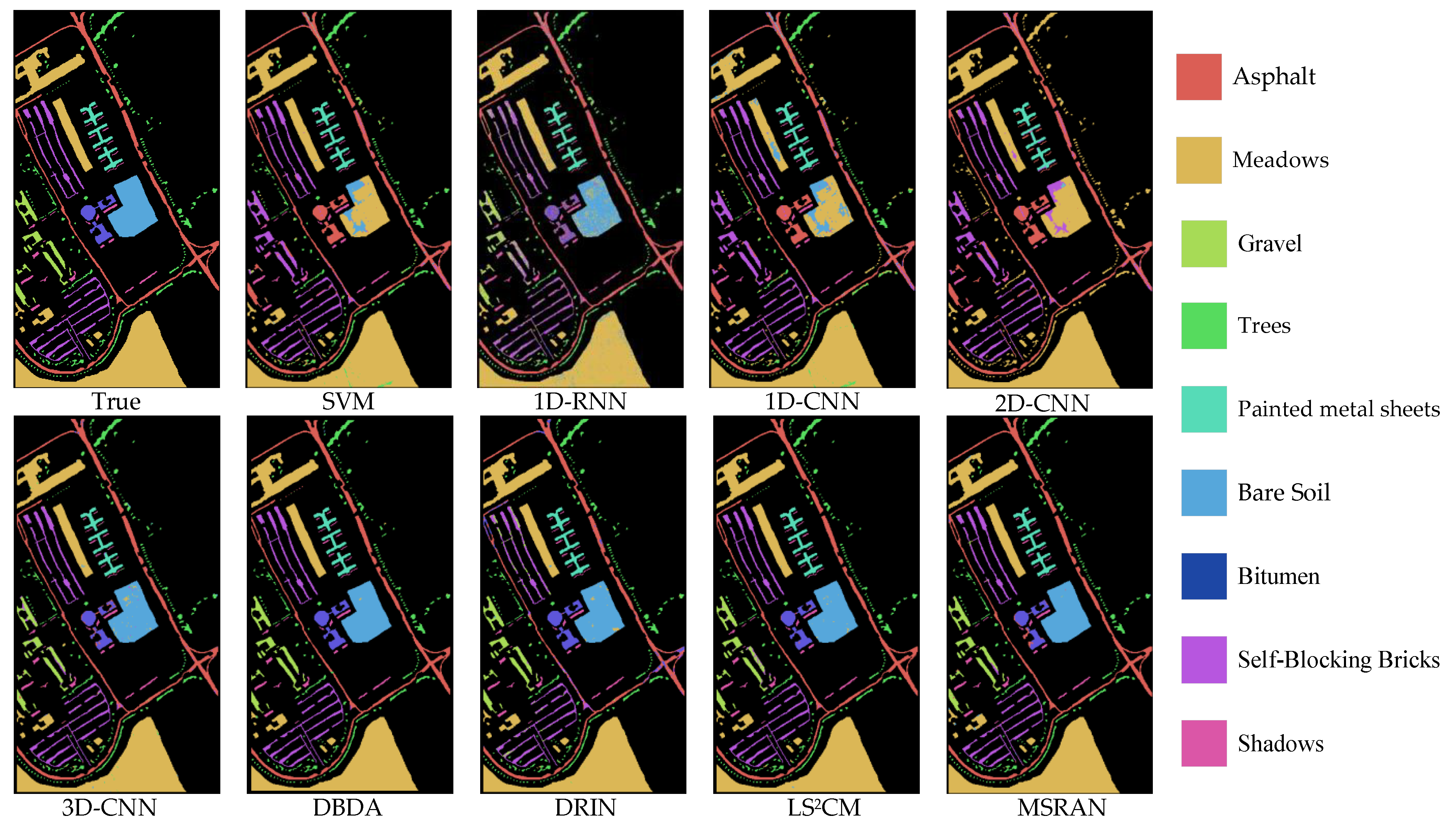
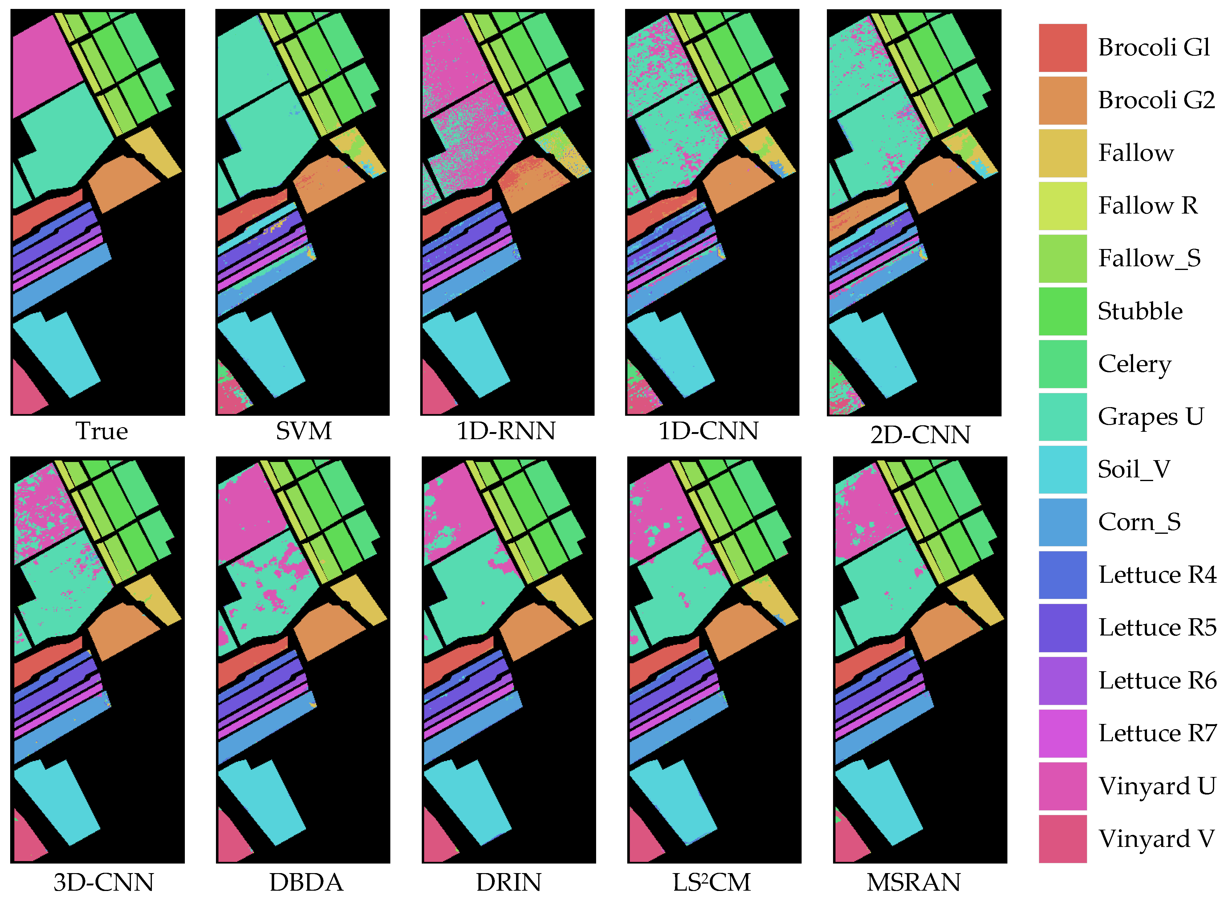
In visual comparisons, classification maps are generated by these methods on the PU, SV, and WHLK datasets, as depicted in Figure 10, Figure 11 and Figure 12. As observed, the maps from the DBDA, DRIN, LS²CM, and MSRAN align more closely with the actual ground conditions, particularly for the classification map of the proposed MSRAN method, which exhibits superior visual accuracy. Conversely, the classification maps from other methods are less precise. While some methods perform well with larger sample sizes, they struggle with smaller, more dispersed samples, such as the scattered Asphalt and Trees in the PU dataset, as shown in Figure 10. Samples that are close to, or even coincident with, edge pixels, such as LettuceR4 in the SV dataset of Figure 11 and Roads and Houses in the WHLK dataset of Figure 12, do not perform well. In contrast, the proposed MSRAN method excels in classes with a high percentage of boundary samples, as shown in the high-resolution WHLK dataset, where it effectively managed complex samples like Roads and Houses and Mixed Weed along Riverbanks with intricate boundary challenges.

Overall, the proposed MSRAN method enhances the spectral features of the central pixel and extracts multi-level fine-grained spatial details, which cooperates with the dual-path residual attention mechanism to screen effective features. By removing the redundant feature interference and minimizing the interference between surrounding pixels, the proposed MSRAN method enables the accurate classification of land cover types in areas with complex spatial distribution, particularly for the areas with scattered and boundary samples.

3.3.3. Impacts of Different Training Ratios

Figure 13 displays the OA values of various models with different proportions of training samples. Considering the varying total number of samples and the stability of the models under exposure to different proportions, 3%, 5%, 7%, and 10% of the training samples were randomly selected for the PU and SV datasets, while 0.5%, 1%, 3%, and 7% were chosen for the WHLK dataset. Overall, it is observed that, even with a limited number of training samples, it still achieves satisfactory classification results. As the number of training samples increases, all methods show a growth trend for performance across these three datasets. Notably, the proposed MSRAN method demonstrates a stable growth trend, further affirming its robustness.

These findings suggest that MSRAN is particularly effective in scenarios with the common challenge of limited training data for HSI classification. Its ability to maintain stable performance improvements with increasing amounts of training data highlights its potential for use in various applications, particularly in areas where collecting extensive training samples is challenging or impractical. The robustness of MSRAN in these contexts underscores its suitability for real-world applications and its effectiveness for harnessing limited data for accurate classification.

4. Conclusions

Traditional convolutional neural network methods often face challenges with feature extraction, particularly in terms of spatial and spectral features influencing each other and the poor extraction of features when there are few samples with multiple edges. This paper introduced a novel method for HSI classification, the Dual-Branch Multi-Scale Spectral–Spatial Residual Attention Network. This approach employs two branches to extract spatial features with different granularities and enhance central-pixel spectral features. It utilizes spatial residual attention and spectral residual attention to refine the extracted spectral–spatial features. Finally, these features are fused and classified using a Softmax classifier for HSIs. Extensive experimental evaluations demonstrated that this method is highly competitive. The dual-branch structure allows for more effective and independent extraction of spatial and spectral features, addressing the limitations of traditional CNN methods. The use of residual attention mechanisms further enhances feature extraction, particularly for complex samples with multiple edges or a limited quantity. The final fusion of these features ensured a comprehensive representation of the data, leading to an improved classification performance. Overall, the MSRAN method provides higher accuracy and robustness for hyperspectral image classification under different scenarios and conditions.

References

1. Wu, Q.; Wu, Y.; Li, Y.; Huang, W. Improved YOLOv5s With Coordinate Attention for Small and Dense Object Detection From Optical Remote Sensing Images. IEEE J. Sel. Top. Appl. Earth Observ. Remote Sens. 2023. [Google Scholar] [CrossRef]
2. Mahlein, A.; Oerke, E.; Steiner, U.; Dehne, H. Recent Advances in Sensing Plant Diseases for Precision Crop Protection. Eur. J. Plant Pathol. 2012, 133, 197–209. [Google Scholar] [CrossRef]
3. Lacar, F.M.; Lewis, M.M.; Grierson, I.T. Use of Hyperspectral Imagery for Mapping Grape Varieties in the Barossa Valley. In Proceedings of the International Geoscience and Remote Sensing Symposium, Sydney, NSW, Australia, 9–13 July 2001; Volume 6, pp. 2875–2877. [Google Scholar]
4. Murphy, R.; Schneider, S.; Monteiro, S. Consistency of Measurements of Wavelength Position from Hyperspectral Imagery: Use of the Ferric Iron Crystal Field Absorption at ∼900 nm as an Indicator of Mineralogy. IEEE Trans. Geosci. Remote Sens. 2014, 52, 2843–2857. [Google Scholar] [CrossRef]
5. Van Der Meer, F. Analysis of Spectral Absorption Features in Hyperspectral Imagery. Int. J. Appl. Earth Obs. Geoinf. 2004, 5, 55–68. [Google Scholar] [CrossRef]
6. Datt, B.; McVicar, T.; Van Niel, T.; Jupp, D.; Pearlman, J. Preprocessing EO-1 Hyperion Hyperspectral Data to Support the Application of Agricultural Indexes. IEEE Trans. Geosci. Remote Sens. 2003, 41, 1246–1259. [Google Scholar] [CrossRef]
7. Zhuang, L.; Wang, J.; Bai, L.; Jiang, G.; Sun, S.; Yang, P.; Wang, S. Cotton Yield Estimation Based on Hyperspectral Remote Sensing in Arid Region of China. Trans. Chin. Soc. Agric. Eng. 2011, 27, 176–181. [Google Scholar]
8. Hestir, E.; Brando, V.; Bresciani, M.; Giardino, C.; Matta, E.; Villa, P.; Dekker, A. Measuring Freshwater Aquatic Ecosystems: The Need for a Hyperspectral Global Mapping Satellite Mission. Remote Sens. Environ. 2015, 167, 181–195. [Google Scholar] [CrossRef]
9. Zhang, P.; Lu, Q.; Hu, X.; Gu, S.; Yang, L.; Min, M.; Chen, L.; Xu, N.; Sun, L.; Bai, W.; et al. Latest Progress of the Chinese Meteorological Satellite Program and Core Data Processing Technologies. Adv. Atmos. Sci. 2019, 36, 1027–1045. [Google Scholar] [CrossRef]
10. Fang, Y.; Xu, L.; Chen, Y.; Zhou, W.; Wong, A.; Clausi, D.A. A Bayesian Deep Image Prior Downscaling Approach for High-Resolution Soil Moisture Estimation. IEEE J. Sel. Top. Appl. Earth Observ. Remote Sens. 2022, 15, 4571–4582. [Google Scholar] [CrossRef]
11. Pang, Y.; Li, Z.; Ju, H.; Lu, H.; Jia, W.; Si, L.; Guo, Y.; Liu, Q.; Li, S.; Liu, L.; et al. LiCHy: The CAF’s LiDAR, CCD and Hyperspectral Integrated Airborne Observation System. Remote Sens. 2016, 8, 398. [Google Scholar] [CrossRef]
12. Guo, A.; Huang, W.; Dong, Y.; Ye, H.; Ma, H.; Liu, B.; Wu, W.; Ren, Y.; Ruan, C.; Geng, Y. Wheat Yellow Rust Detection Using UAV-Based Hyperspectral Technology. Remote Sens. 2021, 13, 123. [Google Scholar] [CrossRef]
13. Della, C.; Bekit, A.; Lampe, B.; Chang, C.-I. Hyperspectral Image Classification Via Compressive Sensing. IEEE Trans. Geosci. Remote Sens. 2019, 57, 8290–8303. [Google Scholar] [CrossRef]
14. Zhao, P.; Tang, Y.; Li, Z. Wood Species Recognition with Microscopic Hyper-spectral Imaging and Composite Kernel SVM. Spectrosc. Spect. Anal. 2019, 39, 3776–3782. [Google Scholar]
15. Xia, J.; Yokoya, N.; Iwasaki, A. Hyperspectral Image Classification with Canonical Correlation Forests. IEEE Trans. Geosci. Remote Sens. 2017, 55, 421–431. [Google Scholar] [CrossRef]
16. Peng, J.; Li, L.; Tang, Y. Maximum Likelihood Estimation-based Joint Sparse Representation for the Classification of Hyperspectral Remote Sensing Images. IEEE Trans. Neural Netw. Learn. Syst. 2019, 30, 1790–1802. [Google Scholar] [CrossRef] [PubMed]
17. Boulch, A.; Audebert, N.; Dubucq, D. Autoencodeurs Pour La Visualisation D’images Hyperspectrales. In Proceedings of the 25th Colloque Gretsi, Juan-les-Pins, France, 5–8 September 2017. [Google Scholar]
18. Chen, Y.; Zhao, X.; Jia, X. Spectral–Spatial Classification of Hyperspectral Data Based on Deep Belief Network. IEEE J. Sel. Top. Appl. Earth Obs. Remote Sens. 2015, 8, 2381–2392. [Google Scholar] [CrossRef]
19. Mou, L.; Ghamisi, P.; Zhu, X.X. Deep Recurrent Neural Networks for Hyperspectral Image Classification. IEEE Trans. Geosci. Remote Sens. 2017, 55, 3639–3655. [Google Scholar] [CrossRef]
20. Hu, W.; Huang, Y.; Wei, L.; Zhang, F.; Li, H. Deep Convolutional Neural Networks for Hyperspectral Image Classification. J. Sens. 2015, 2015, 258619. [Google Scholar] [CrossRef]
21. Sharma, V.; Diba, A.; Tuytelaars, T.; Van Gool, L. Hyperspectral CNN for Image Classification and Band Selection, with Application to Face Recognition; Technical Report KUL/ESAT/PSI/1604; KU Leuven, ESAT: Leuven, Belgium, 2016. [Google Scholar]
22. Yang, J.; Zhao, Y.; Chan, J. Learning and Transferring Deep Joint Spectral–spatial Features for Hyperspectral Classification. IEEE Trans. Geosci. Remote Sens. 2017, 55, 4729–4742. [Google Scholar] [CrossRef]
23. Li, Y.; Zhang, H.; Shen, Q. Spectral–Spatial Classification of Hyperspectral Imagery with 3D Convolutional Neural Network. Remote Sens. 2017, 9, 67. [Google Scholar] [CrossRef]
24. Chen, Y.; Jiang, H.; Li, C.; Jia, X.; Ghamisi, P. Deep Feature Extraction and Classification of Hyperspectral Images Based on Convolutional Neural Networks. IEEE Trans. Geosci. Remote Sens. 2016, 54, 6232–6251. [Google Scholar] [CrossRef]
25. Zhong, Z.; Jonathan, L. Spectral-spatial Residual Network for Hyperspectral Image Classification: A 3-D Deep Learning Framework. IEEE Trans. Geosci. Remote Sens. 2018, 56, 847–858. [Google Scholar] [CrossRef]
26. Qi, Y.F.; Chen, J.; Huo, Y.L. Hyperspectral Image Classification Algorithm Based on multi-scale Convolutional Neural Network. Infrared Tech. 2020, 42, 855–862. [Google Scholar]
27. Li, R.; Zheng, S.; Duan, C.; Yang, Y.; Wang, X. Classification of Hyperspectral Image Based on Double-Branch Dual-Attention Mechanism Network. Remote Sens. 2020, 12, 582. [Google Scholar] [CrossRef]
28. Meng, Z.; Zhao, F.; Liang, M.; Xie, W. Deep Residual Involution Network for Hyperspectral Image Classification. Remote Sens. 2021, 13, 3055. [Google Scholar] [CrossRef]
29. Zhang, C.; Li, G.D.; Du, S.H. Multi-Scale Dense Networks for Hyperspectral Remote Sensing Image Classification. IEEE Trans. Geosci. Remote Sens. 2019, 57, 9201–9222. [Google Scholar] [CrossRef]
30. He, N.; Paoletti, M.E.; Haut, J.M.; Fang, L.; Li, S.; Plaza, A.; Plaza, J. Feature Extraction with multi-scale Covariance Maps for Hyperspectral Image Classification. IEEE Trans. Geosci. Remote Sens. 2019, 57, 755–769. [Google Scholar] [CrossRef]
31. Woo, S.; Park, J.; Lee, J.Y. Cbam: Convolutional Block Attention Module. In Proceedings of the European Conference on Computer Vision, Munich, Germany, 8–14 September 2018; pp. 3–19. [Google Scholar]
32. Cheng, R.J.; Yang, Y.; Li, L.W. Lightweight Residual Network Based on Depthwise Separable Convolution for Hyperspectral Image Classification. Acta Opt. Sin. 2023, 43, 1228010. [Google Scholar] [CrossRef]
33. Hyperspectral Remote Sensing Scenes. Available online: https://www.ehu.eus/ccwintco/index.php/Hyperspectral%20Remote%20Sensing%20Scenes (accessed on 11 January 2023).
34. Zhong, Y.; Hu, X.; Luo, C.; Wang, X.; Zhao, J.; Zhang, L. WHU-Hi: UAV-borne Hyperspectral with High Spatial Resolution (H2) Benchmark Datasets and Classifier for Precise Crop Identification based on Deep Convolutional Neural Network with CRF. Remote Sens. Environ. 2020, 250, 112012. [Google Scholar] [CrossRef]
35. Wu, Q.G.; Liu, Z.C.; He, M.K. Fusion of MS3D-CNN and Attention Mechanism for Hyperspectral Image Classification. J. Chongqing Inst. Technol. 2023, 37, 173–182. [Google Scholar]
36. Yang, Z.H.; Li, Z.X.; Han, J.F. The Hughes Phenomenon in Hyperspectral Analysis and the Application of the Lowpass Filter. Acta Geod. Cartogr. Sin. 2004, 4, 253–255+258. [Google Scholar]
37. Thompson, W.D.; Walter, S.D. A Reappraisal of the Kappa Coefficient. J. Clin. Epidemiol. 1988, 41, 949–958. [Google Scholar] [CrossRef] [PubMed]
38. Meng, Z.; Jiao, L.; Liang, M.; Zhao, F. A Lightweight Spectral-Spatial Convolution Module for Hyperspectral Image Classification. IEEE Geosci. Remote Sens. Lett. 2022, 19, 5505105. [Google Scholar] [CrossRef]
Figure 1. Overall architecture of the proposed MSRAN for HSI classification.
Electronics 13 00262 g001
Figure 2. Spectral feature extraction and optimization branch.
Electronics 13 00262 g002
Figure 3. Spectral residual attention structure.
Electronics 13 00262 g003
Figure 4. Structure of the spatial feature extraction and optimization module.
Electronics 13 00262 g004
Figure 5. Structure of the spatial residual attention.
Electronics 13 00262 g005
Figure 6. Feature fusion and classification module.
Electronics 13 00262 g006
Figure 7. Pseudo-color image and ground truth image of the PU dataset.
Electronics 13 00262 g007
Figure 8. Pseudo-color image and ground truth image of the SV dataset.
Electronics 13 00262 g008
Figure 9. Pseudo-color image and ground truth image of the WHLK dataset.
Electronics 13 00262 g009
Figure 10. Classification maps of the PU dataset with different methods.
Electronics 13 00262 g010
Figure 11. Classification maps of the SV dataset with different methods.
Electronics 13 00262 g011
Figure 12. Classification maps of the WHLK dataset with different methods.
Electronics 13 00262 g012
Figure 13. Classification results versus different percentages of training samples for the three datasets. (a) PU. (b) SA. (c) WHLK.
Electronics 13 00262 g013