Abstract
With the increasing popularity of cloud-native architectures and containerized applications, Kubernetes has become a critical platform for managing these applications. However, Kubernetes still faces challenges when it comes to resource management. Specifically, the platform cannot achieve timely scaling of the resources of applications when their workloads fluctuate, leading to insufficient resource allocation and potential service disruptions. To address this challenge, this study proposes a predictive auto-scaling Kubernetes Operator based on time series forecasting algorithms, aiming to dynamically adjust the number of running instances in the cluster to optimize resource management. In this study, the Holt–Winter forecasting method and the Gated Recurrent Unit (GRU) neural network, two robust time series forecasting algorithms, are employed and dynamically managed. To evaluate the effectiveness, we collected workload metrics from a deployed RESTful HTTP application, implemented predictive auto-scaling, and assessed the differences in service quality before and after the implementation. The experimental results demonstrate that the predictive auto-scaling component can accurately predict the future trend of the metrics and intelligently scale resources based on the prediction results, with a Mean Squared Error (MSE) of 0.00166. Compared to the deployment using a single algorithm, the cold start time is reduced by 1 h and 41 min, and the fluctuation in service quality is reduced by 83.3%. This process effectively enhances the quality of service and offers a novel solution for resource management in Kubernetes clusters.
1. Introduction
The evolution of cloud computing has been significantly shaped by virtualization technologies such as KVM and Xen, which have revolutionized the utilization and management of computing resources [1]. As technology has advanced, containerization has emerged as a leading paradigm for deploying and managing applications, due to its lightweight, portable, and efficient nature [2]. Containerization allows applications and their dependencies to be packaged into standalone units, enabling seamless execution across various environments [2,3]. This development has paved the way for Kubernetes, an open-source platform that orchestrates these containers, ensuring efficient and reliable application deployment and management [4,5].
For Kubernetes, its automatic scaling capability is one of its core features [6]. Through automatic scaling, Kubernetes can flexibly allocate resources for different business objects to ensure stable operation and resource efficiency. Kubernetes mainly provides two passive scaling methods: Horizontal Pod Auto-scaling (HPA) and Vertical Pod Auto-scaling (VPA) [7]. HPA scales by increasing or decreasing the number of Pod replicas, while VPA scales by adjusting the resource quotas of each Pod. In cloud-native environments, HPA is the primary scaling method [8]. However, related research indicates that the reactive scaling methods provided by Kubernetes trigger scaling operations only when metrics reach certain thresholds, which results in response delays and can impact the stability of the business, and can even lead to large-scale service interruptions in some cases [7,9].
In order to address potential issues caused by the traditional passive scaling, numerous studies have emerged. Some of these studies are dedicated to optimizing passive scaling strategies, while others explore methods of active scaling [10,11,12,13]. However, these optimization strategies often rely on specific, singular algorithms, and the majority of research primarily focuses on applications in virtualized environments. Meanwhile, related studies in containerized environments are still in the early stages.
To address the challenges of elastic resource scaling in containerized environments, this study proposes a Kubernetes scaling strategy based on time-series forecasting. Machine learning predictive methods, which have been widely applied across various fields [14,15], offer effective solutions such as traditional Recurrent Neural Networks (RNN) and Long Short-Term Memory (LSTM) for time-series forecasting [16]. Therefore, the application of these methods to Kubernetes predictive scaling holds promising potential. To adapt to containerized scenarios, we developed an automatic scaling system using the Kubernetes Operator mode. To enhance its versatility, the system allows for the integration of multiple predictive models. In addition to the Holt–Winter and GRU models integrated within the system, users can expand to more models through a generic interface to adapt to different business scenarios. By monitoring the runtime metrics of business objects and predicting their future trends, we can execute scaling operations before resource demand peaks, thus ensuring the stable operation of the business.
The experimental results demonstrate that the predictive scaling operator can effectively supervise applications within the Kubernetes cluster, collect application metric data, and perform predictive scaling. By proactively expanding resources before the arrival of peak loads, it significantly enhances the stability of the applications. Simultaneously, it contracts resources during low-load periods, thus preventing resource wastage. This method provides a new perspective on resource management within the Kubernetes environment, allowing for more precise resource allocation. It has made a certain contribution to improving the efficiency and performance of applications within the Kubernetes cluster.
2. Related Work
Numerous studies have emerged that address the issues of potential degradation in application service quality or resource wastage caused by the traditional HPA scaling methods in Kubernetes. These can be principally categorized into reactive and proactive scaling methods.
HPA represents a typical reactive scaling method, setting the metrics and thresholds for auto-scaling. When the application’s metrics reach the corresponding thresholds, HPA triggers the auto-scaling operation. Some studies, building on horizontal scaling, have improved this threshold-based auto-scaling method by optimizing threshold selection and integrating more auto-scaling methods.
In [17], the authors proposed a new scaling framework, Libra, which combines Kubernetes’ HPA and VPA to more rationally determine the resource upper limit of each pod, thereby achieving more precise horizontal scaling. The experimental results demonstrate that Libra performs better in CPU resource allocation compared to traditional scaling methods.
Alibaba Cloud has developed a new scaling component, Kubernetes Pod Autoscaler (KPA) [18], which incorporates various modes, such as stable and emergency modes. Depending on the application’s status, this component can switch between different modes, each with distinct scaling thresholds. Through this approach, KPA achieves more flexible reactive scaling.
The open-source component, Kubernetes Event-Driven Auto-scaling (KEDA), transforms threshold-based reactive scaling into event-driven scaling [19]. By monitoring specific events of the application, it allocates resources to the application, making the application’s resource scaling more flexible. Experimental evidence shows that it can effectively optimize application performance in a cloud-native environment.
However, reactive auto-scaling exhibits a certain degree of latency. Auto-scaling operations are only triggered when specified thresholds are reached or specific events are captured. For some applications with longer startup times, the initialization process may take considerable time after the auto-scaling command is issued. This can impact the stability of the service during this phase and may significantly affect service quality.
In contrast, proactive auto-scaling is based on certain predictive algorithms that are used to calculate the load trend of the application and complete auto-scaling operations in advance, compensating for the shortcomings of reactive scaling. There are some noteworthy studies on this topic.
In [20], the authors proposed an auto-scaling architecture based on machine learning. Using load data obtained from the load balancer, the system employs the LSTM model to predict the future load trend of the application. The experimental results show that, compared to the Autoregressive Integrated Moving Average (ARIMA) and Artificial Neural Networks (ANN) models, the LSTM model has a lower prediction loss value.
In [21], a predictive auto-scaling method based on Bidirectional LSTM (Bi-LSTM) was proposed. The experimental results indicate that this model possesses a higher accuracy compared to the LSTM model.
In [22], the authors constructed an auto-scaling component that uses Prometheus to collect and store custom metrics gathered within the cluster. In terms of metric analysis, the authors used ARIMA, LSTM, Bi-LSTM, and Transformer models to predict the number of HTTP requests received by the application. Experimental comparisons revealed that the Transformer model provided the best accuracy in workload prediction.
However, learning-based algorithms require a large amount of data for training, taking a long time to prepare the model in the context of real-time data collection. Another study proposed an autoscale controller that includes both reactive and predictive controllers. In the predictive controller, the Autoregressive Moving Average (ARMA) statistical model is used to predict the requests received by the application [10]. Although this type of algorithm does not require a large amount of historical data, its accuracy still needs to be improved compared to that of learning-based algorithms.
Evidently, while the reactive scaling method is simple to implement, it does not effectively address the issue of scaling lag. On the other hand, although proactive scaling methods can complete scaling operations in advance, they require substantial data support. Moreover, existing studies typically only activate one prediction model, failing to fully exploit the advantages of different models to adapt to various scenarios.
Inspired by previous studies and in order to accommodate more use cases, ensure predictions can be made even with limited data, and achieve higher accuracy predictions with ample data, the predictive scaling method proposed in this paper employs and manages multiple prediction models. It also supports users in adding custom prediction models and parameter configurations.
3. Methodology
3.1. Time Series Forecasting Algorithms
3.1.1. Holt–Winter Algorithm
The Holt–Winter algorithm, also known as triple exponential smoothing, is a prevalent method for forecasting time series data with both seasonal and trend components. Unlike simple exponential smoothing, the Holt–Winter algorithm incorporates both trend and seasonal factors, aligning its predictions more closely with real-world scenarios [23].
At its core, the Holt–Winter algorithm forecasts future data by applying exponential weighted smoothing to historical data. This approach assigns higher weights to recent data and gradually reduces the reliance on older data, allowing the model to adapt to changes in the time series dynamically.
The Holt–Winter algorithm comprises three main components: the level, trend, and seasonal components. These components collectively form the forecasting framework of the Holt–Winter model. The level and trend components describe the basic shape of the time series, while the seasonal component captures the patterns of change across different seasons. This combination makes the Holt–Winter algorithm particularly effective for forecasting seasonal time series data with high prediction accuracy. The specific implementation formulas of the model are as follows:
Equations (1)–(4) represent the formulas for the level component, trend component, seasonal component, and prediction, respectively. In the formulas mentioned above, represents the level at time x, represents the trend at time x, is the actual observed value at time x, represents the seasonal component at time x, is the seasonal component from the previous quarter, is the seasonal component for m periods into the future, and represents the forecasted value for m periods into the future. Also, these four formulas have parameters , , and , all of which are hyperparameters. Their values need to be determined through an optimization process to achieve the best forecasting performance.
In summary, the Holt–Winter algorithm, through smoothing of historical data and consideration of time series’ level, trend, and seasonal characteristics, accomplishes the forecasting of future data. Its major advantage is that it does not require complex training processes; you only need to set the hyperparameters, and you can directly make predictions. This makes the Holt–Winter algorithm widely valuable in time series forecasting.
3.1.2. Gated Recurrent Units
Gated Recurrent Unit (GRU) is a popular recurrent neural network architecture introduced by Cho and others in 2014 [24]. The design of the GRU network structure aims to address the challenges faced by traditional Recurrent Neural Networks (RNNs) in handling long-term dependencies while maintaining a more concise computational complexity compared to Long Short-Term Memory (LSTM) networks [25].
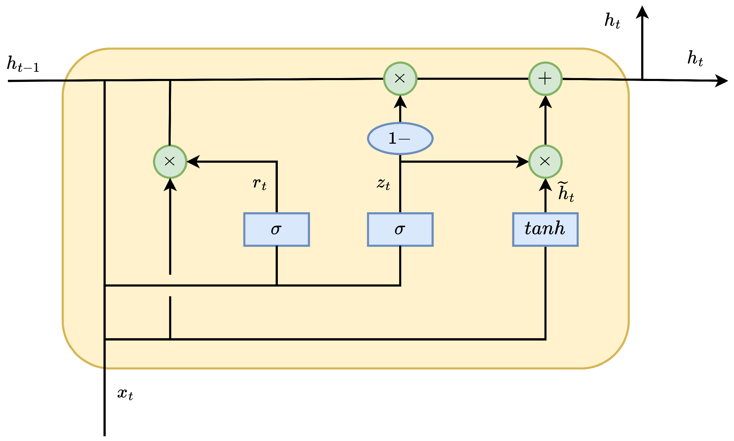
The key feature of GRU networks is the introduction of two structures: the update gate and the reset gate. The update gate determines how much of the previous hidden state information should be retained when generating the current hidden state, while the reset gate controls the influence of past hidden state information when generating the candidate hidden state. These two gating mechanisms enable GRU to effectively capture long-term dependencies in time series data. The design effectively resolves the gradient explosion problem in RNNs [26].
The unit structure of GRU is as shown in the diagram (Figure 1).
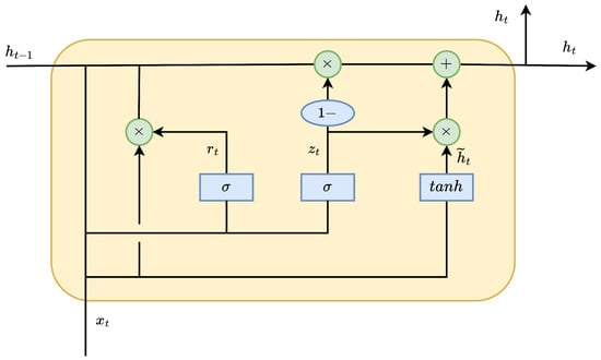
Figure 1.
GRU Unit Structure Diagram.
The corresponding forward propagation equations are as follows.
GRU uses different subscripts to represent its weight matrices, where x corresponds to input, r represents the update gate, h stands for the hidden state, and z denotes the reset gate. Additionally, GRU includes bias vectors , and , which correspond to different structural components. By summing the parameters of the three gates, the total number of parameters for the GRU can be obtained as: .
Furthermore, GRU is more concise compared to LSTM, primarily because GRU has only two gating mechanisms while LSTM has three. This results in GRU having fewer parameters than LSTM, reducing the model’s computational complexity and training difficulty. Simultaneously, in terms of accuracy, in some non-complex scenarios, GRU and LSTM achieve similar levels of precision [24]. Therefore, for tasks that require efficient training with limited computational resources, GRU is often a better choice.
3.2. Predictive Model Management Method
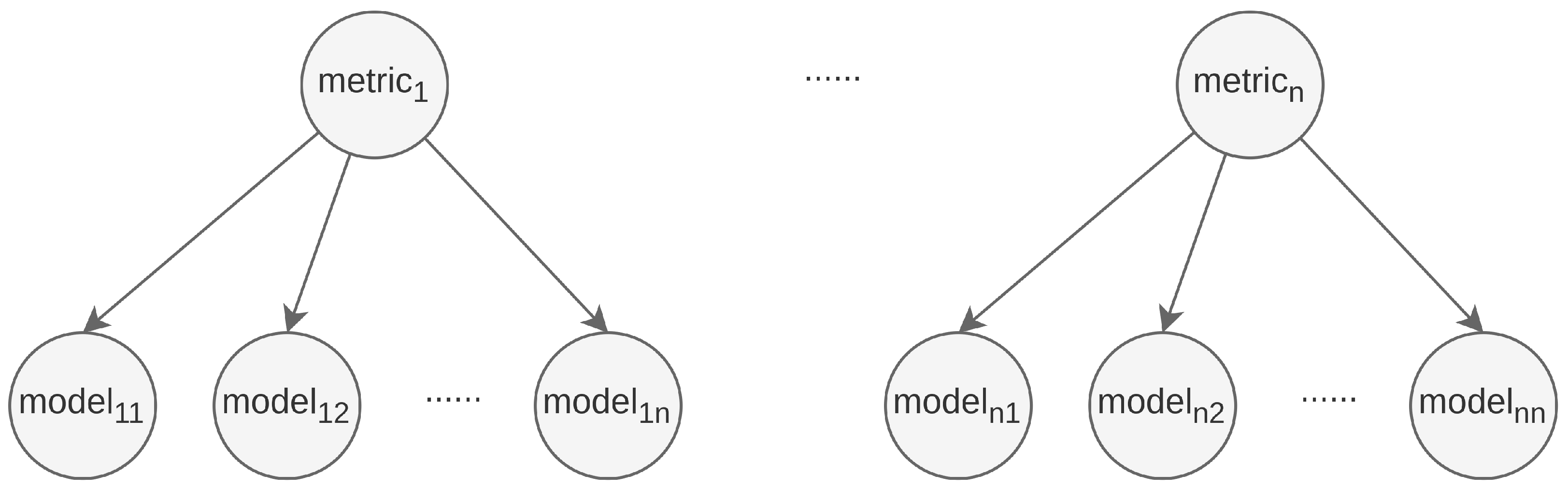
To seamlessly integrate with Kubernetes clusters, this study designed and implemented a custom resource definition (CRD) and a corresponding Kubernetes Operator for fine-grained control. The CRD includes information about the data source interface for data acquisition, the metrics to be monitored, and the prediction models to be used for prediction. Each metric supports multiple prediction models for prediction (Figure 2).
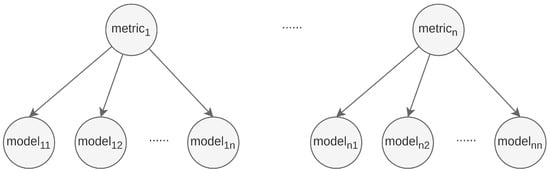
Figure 2.
Metric-Model Correspondence Diagram.
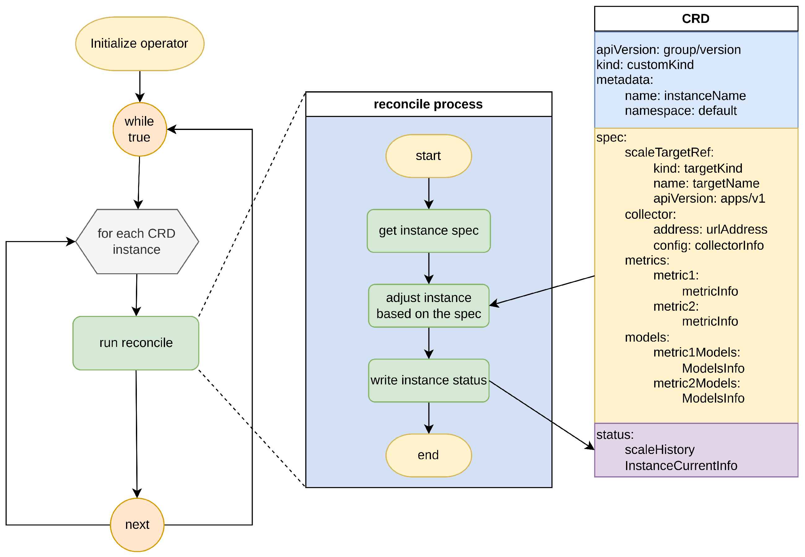
Users can define monitoring metrics and prediction models through a YAML configuration file. In the metric configuration, users can specify the query expression, weight, and all relevant prediction models corresponding to the metric. In the prediction model configuration, users need to provide the category of the prediction model, whether it needs to be trained, and the hyperparameter configuration. Once the YAML configuration file has been created, users send it to the Kubernetes API Server. When the API Server receives the YAML configuration file, it triggers the corresponding Operator’s reconciling process. The process diagram is as follows (Figure 3).
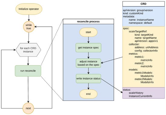
Figure 3.
Operator reconcile process.
Upon completion of initialization, the Operator continuously receives information about CRD instances that need to be processed from the API Server, and performs Reconcile operations on each CRD object. Initially, the Operator obtains the spec information for each CRD object, which is provided by the user-defined YAML configuration file, enabling the Operator to identify the desired state of the CRD object. To obtain the current state of the CRD object, the Operator retrieves the current CRD object from the local CRD object cache built during the initialization stage, based on the key value of the CRD object being processed at that moment. It then compares the current state with the desired state, executing a creation operation if the current object does not exist, or a modification operation if both exist. Ultimately, this predictive auto-scaling CRD instance will be deployed in the form of a Pod within the Kubernetes cluster and managed by the cluster.
Notably, during the creation operation, the Operator instantiates the prediction model based on the information and parameters in the spec. The Operator integrates various differently implemented prediction models via communication, currently supporting TCP and UDS protocols. Therefore, during model scheduling, triggering the model and managing different models can be conveniently achieved by invoking the unified abstract interface at the upper layer.
In terms of data support for the prediction model, the Operator will create a Collector based on the data source address and configuration information in the spec. This Collector adopts a global singleton pattern and is shared by all CRD instances. The Collector, based on the PromQL statements contained in the metrics of each instance, initiates corresponding subroutines which query and fetch data from the data source in real-time in the background. All these subroutines are managed by the global Collector. When the prediction model needs data for training or prediction, it obtains the corresponding data from the subroutines managed by the Collector.
Finally, the Operator successfully creates a CRD instance object, establishes a mapping between the metrics and prediction models in the object, and configures the data source to ensure that each model can effectively obtain data from the configured data source.
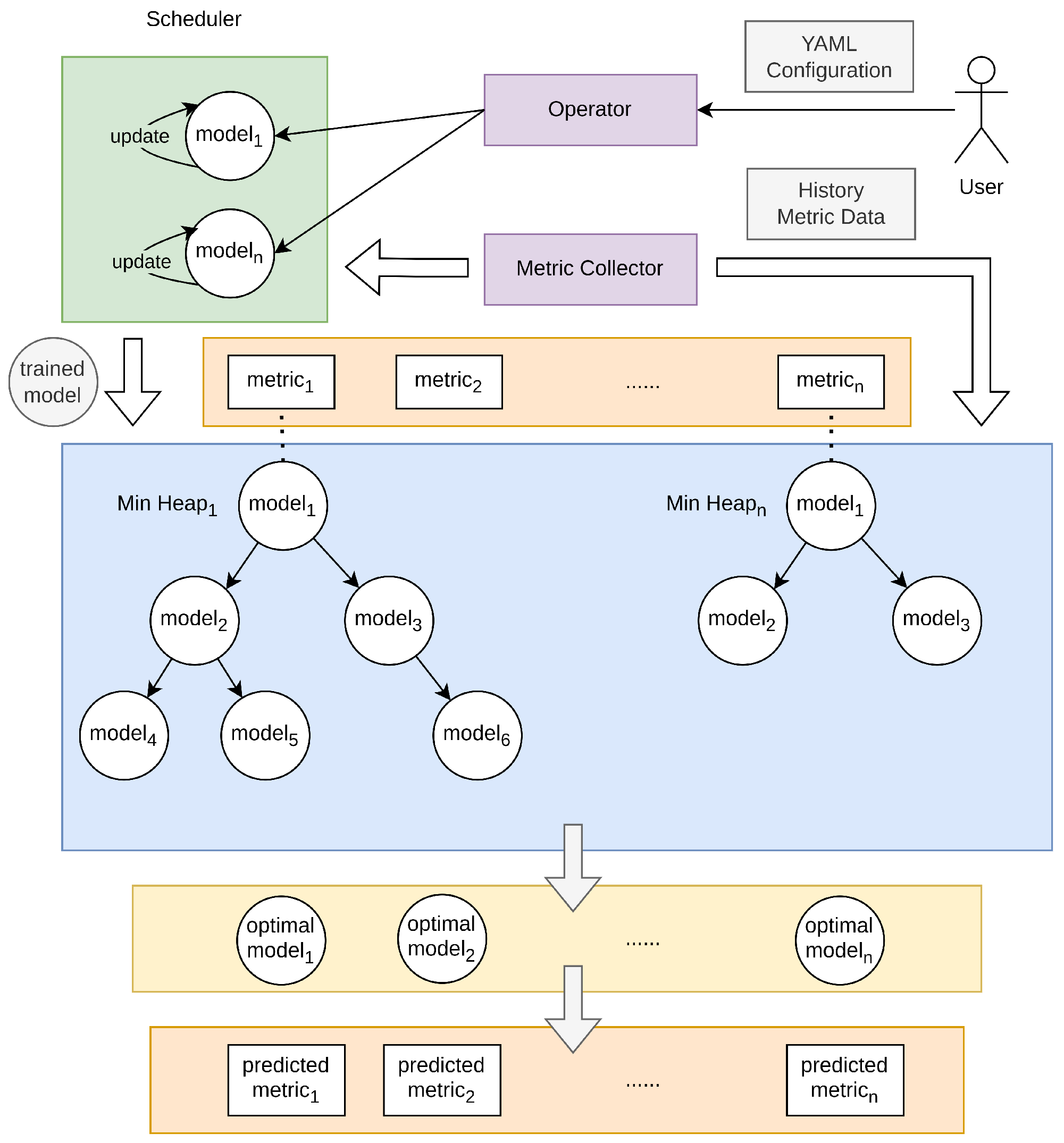
Overall, once the CRD object has been successfully created or modified, the scheduler in the Operator will train or update the models. Then, the Operator will place the model corresponding to each metric in a min-heap sorted by loss value. When a prediction is needed, each metric will use the optimal model at the top of the heap to predict the corresponding metric, and finally obtain the prediction value of each metric. The overall diagram of model management is as follows (Figure 4).
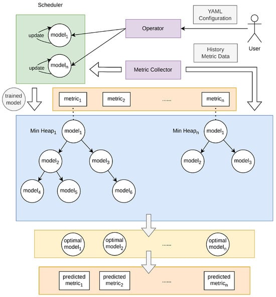
Figure 4.
Model management diagram.
To effectively manage and coordinate models, we have designed and implemented the Scheduler component in the Operator, with its core responsibility being the intelligent management of predictive models input by the user. Once the user inputs relevant models through YAML configuration files, The Scheduler component will initiate two coroutines: the main coroutine and the update coroutine. In the main coroutine, the scheduler first enters an initialization phase. During this phase, the scheduler waits for all non-training models to collect data, with the data volume equal to the sum of input and output dimensions. Subsequently, a simulation prediction is performed on these non-training models, and this prediction does not trigger scaling operations. After obtaining the predicted results, the scheduler compares them with the ground truth, calculates the mean squared error (MSE) for each model, and places the models into the corresponding min-heap based on the MSE value and the associated metrics. Following the conclusion of this phase, the scheduler initiates an update coroutine responsible for training and updating the models.
As for the computational complexity, with the number of metrics as m, and with each metric containing n predictive models, the time complexity for each stage is calculated as follows. Since the initialization complexity of each heap is , the time complexity for constructing the mapping of all indicators and models is . After the initialization stage, the update of each model may adjust its position in the heap. According to the nature of the heap, the time complexity of adjusting a single element is . Therefore, the overall time complexity of model updates is . In the prediction stage, as the top model in the heap is already the optimal model, the time complexity for selecting the model is .
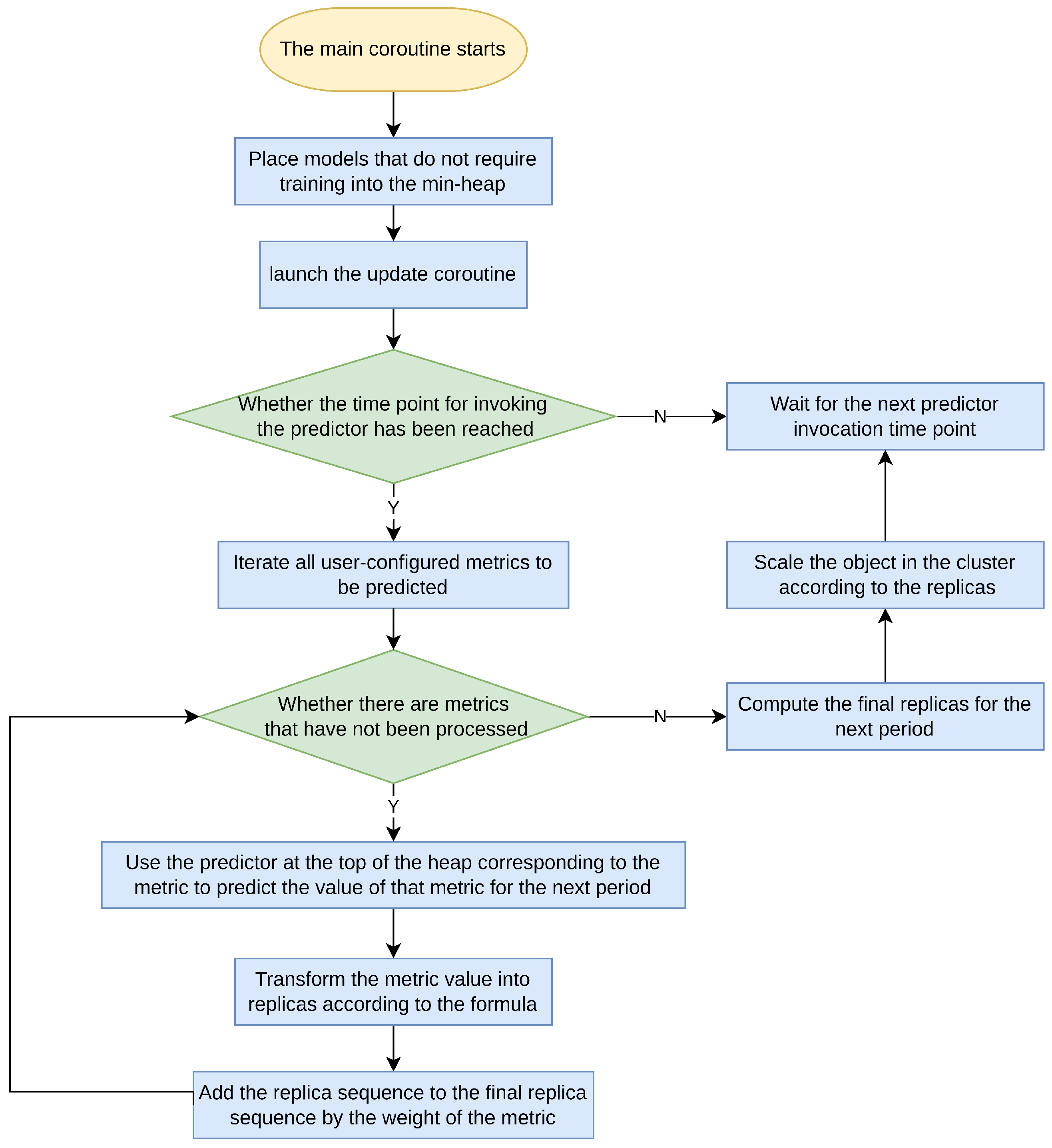
In the main coroutine, the primary function is to periodically trigger the currently available models and make predictions for relevant metrics. It is noteworthy that the output dimensions for all models are set to the same value in the YAML configuration. Therefore, the scheduler’s time interval is configured to match the time length of the output dimensions of all models. This configuration ensures that after each prediction-based scaling operation is triggered, the replicas for the next cycle can be effectively planned, avoiding situations of redundant predictions. The Flowchart of the main coroutine is as follows (Figure 5).

Figure 5.
Flowchart of the main coroutine.
When the Scheduler performs predictions, it selects the model at the top of the min-heap associated with the required predictive metric to ensure that the model being used has the lowest error. Subsequently, the Scheduler uses the historical metric data to make predictions about the trend of the metrics in the next time interval. Once the predicted metrics have been obtained, the scheduler transforms these metrics into the number of replicas according to Formula (9). Subsequently, it scales the corresponding workloads of applications in the cluster (Deployment, StatefulSet, etc.) based on the resulting replica count sequence.
In the above formula, n represents the number of replicas determined based on the predicted metrics, p represents the forecasted metric data, and q represents the target metric data that are obtained from the user-configured YAML file. u represents the the number of copies corresponding to the target metric, with a default value of one, and can be configured in the YAML file.
During the scaling, to avoid frequent fluctuations in workload replicas, if the time interval for replica changes is less than the set minimum action time interval, the Scheduler aggregates the replica sequence. It uses a sliding window with a length equal to the number of time points within a minimum action time window and selects the maximum number of replicas within the window for scaling operations during each slide. This strategy helps maintain the stability of the workload.
The update coroutine is initiated by the main coroutine and is primarily responsible for the training and updating of models. The workflow diagram is shown below (Figure 6).
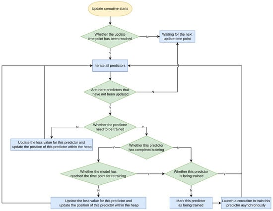
Figure 6.
Flowchart of the update coroutine.
The update coroutine also periodically updates all models, but the interval for this process is different from that in the main coroutine. This interval can be configured by the user in the YAML file and is generally longer than the scheduling interval in the main coroutine. When the update time point is reached, the update coroutine will categorize the models into two types: models that require training and those that do not. For models that do not require training, as is the case during the model initialization phase in the main coroutine, all models that do not require training have already gathered sufficient data for simulated predictions, the update coroutine will directly simulate predictions for all such models. Subsequently, it computes their MSE and adjusts the positions of the models in the heap based on this value.
As for models that require training, the update coroutine checks whether the model has completed training. If the model has finished training but has reached the user-configured retraining time point, the scheduler will retrain the model. Otherwise, it will obtain the model’s latest MSE through a simulated prediction and adjust its position in the heap. For models that have never been trained, the scheduler will initiate their training. It is important to note that during training, as it typically takes a considerable amount of time, the update coroutine internally starts a new coroutine and communicates asynchronously with it through a channel. When the new coroutine receives the training result, the update coroutine receives the message through the channel and places the model in the heap based on the training error and the corresponding metric.
4. Results
In this section, simulation will be conducted to validate the Kubernetes scaling method based on time series forecasting proposed in this research.
4.1. Application Configuration
In order to simulate a real-world environment, the simulation constructed a Kubernetes cluster with one master and three worker nodes. The configuration of the nodes is as follows (Table 1):

Table 1.
Kubernetes cluster specifications.
After building the cluster, the predictive scaling component implemented in this article was extended to the cluster as a Kubernetes Operator. Within the cluster, a simple product detection backend server was developed and deployed, which exposes two HTTP interfaces to the outside. The interfaces are as follows (Table 2):
Table 2.
Server URI List.
The server is deployed in the cluster in the form of a deployment and implements load-balancing capabilities through a service and ingress workload, providing services to the outside world.
To simulate service quality, the server has a rate-limiting mechanism. When the number of requests reaches a certain threshold, it will directly return an HTTP status code of 500 to the client. On the client side, periodic random requests are sent to the server. After receiving requests on the server, Prometheus deployed in the cluster collects request data [27]. The predictive scaling component will use the data collected by Prometheus to perform training and predictions.
The software used in this experiment includes (Table 3):
Table 3.
Software List.
4.2. Experimental Results
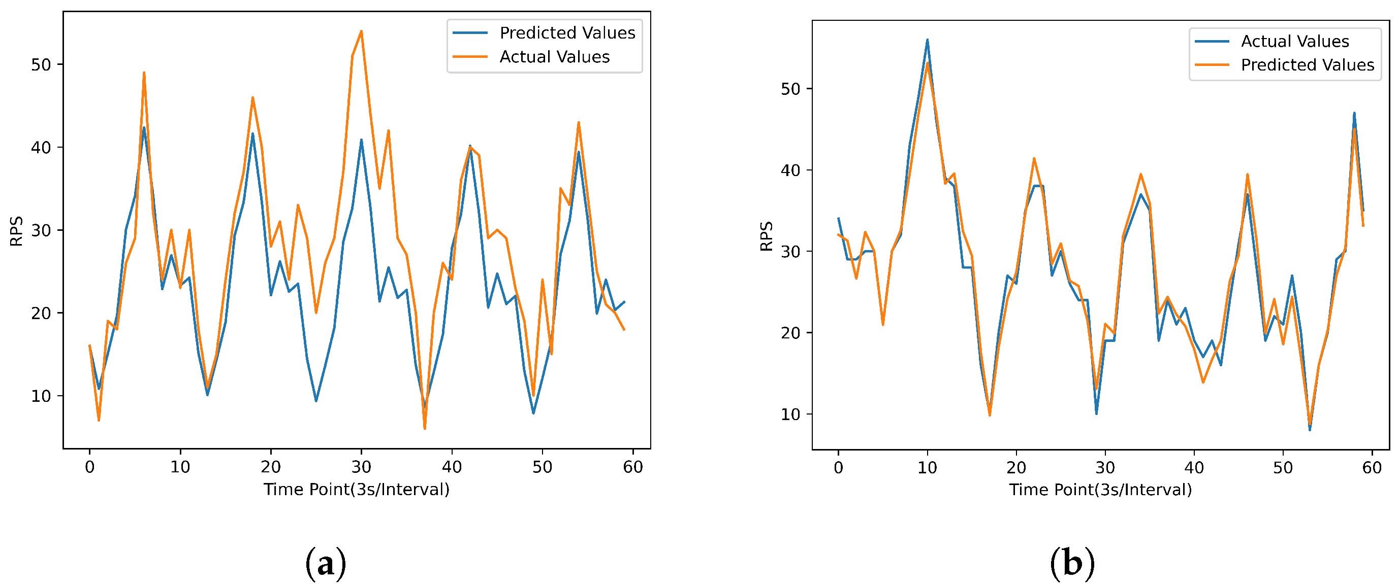
In the experiment, a client process was launched to consistently send HTTP requests to the service deployed in the cluster. These requests were periodic, with the introduction of some random disturbances. Simultaneously, the operator collected the requests received by the service in the cluster. Based on the collected historical data, in the case of the Holt–Winter forecasting algorithm, predictions were made for the future 60 time points using data from the past 120 time points. For GRU, a total of 2000 data points were divided into 1821 sets of data with input dimensions of 120 and output dimensions of 60, and were used as the training dataset. Predictions were made for the future 60 time points based on data from the past 120 time points. The results are as follows (Figure 7):
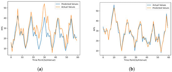
Figure 7.
Predictive results graph. (a) Holt–Winter result. (b) GRU result.
After normalizing the output of the prediction model and the true values, the Mean Squared Error (MSE) is calculated using the following formula:
In this context, stands for Mean Squared Error, n represents the length of the time series, is the actual observed value at time point i, and is the corresponding predicted value. The results are as follows (Table 4):
Table 4.
Comparison of key metrics for two algorithms.
Based on the data in the table, we can observe that compared to deploying only the GRU model, the system’s cold start time, which is the time during data collection and model preparation when the system is unable to function, has decreased by min, or about 1 h and 41 min.
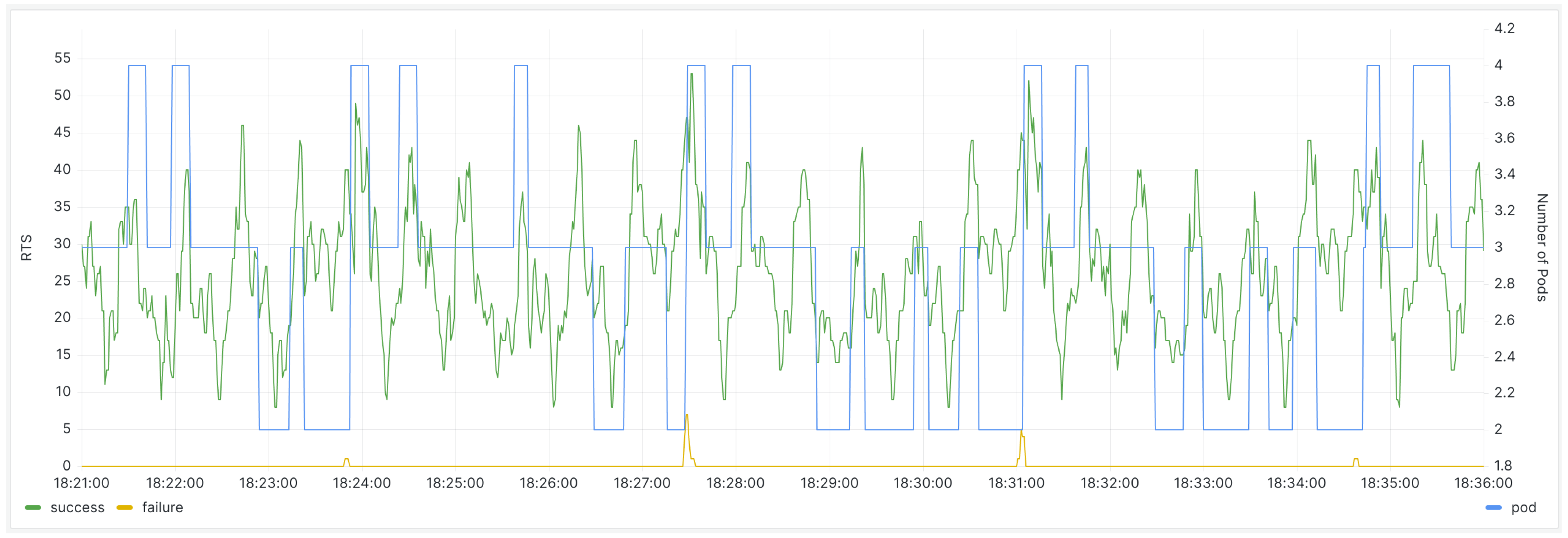
When the predictive scaling component is not deployed in the cluster, the request handling status of the backend server, as well as the number of pods in the Grafana monitoring panel, are as follows (Figure 8):
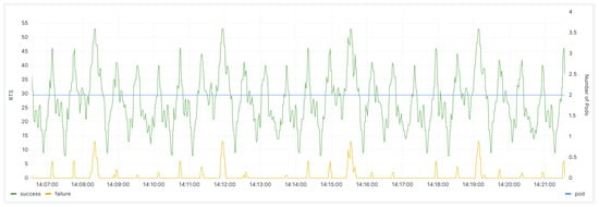
Figure 8.
The monitoring panel for the backend service before the deployment of the scaling component.
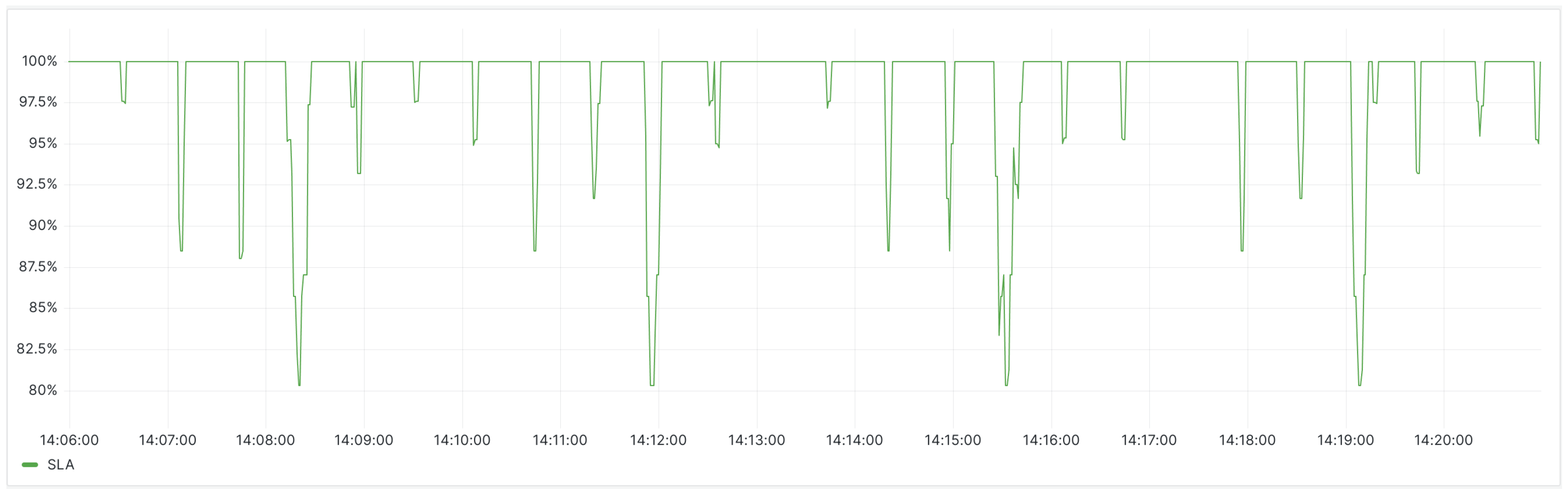
When evaluating the quality of backend business services, we adopted Service-Level Agreements (SLA). SLAs encompass various types, including availability, accuracy, system capacity, and latency, each applicable to different scenarios and with distinct metrics. For instance, availability SLA measures the success rate of API calls to assess the availability of interfaces, accuracy SLA employs the rate of system exception throws as a metric, and capacity SLA uses the maximum number of requests the system can handle as a metric, and so on. As the application monitored in this experiment is a RESTful HTTP service where HTTP status codes indicate the status of interface requests, we chose to assess using SLA for availability. The specific evaluation metric is the ratio of HTTP 200 responses to the total responses, representing the success rate of requests. The SLA is calculated by dividing the number of successfully processed requests by the total number of requests. It can be observed that during peak request times, the SLA reaches 80.3%, indicating that there is still some room for improvement in achieving a highly reliable service quality (Figure 9).
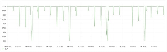
Figure 9.
Before the deployment of the scaling component, the SLA status for the backend service.
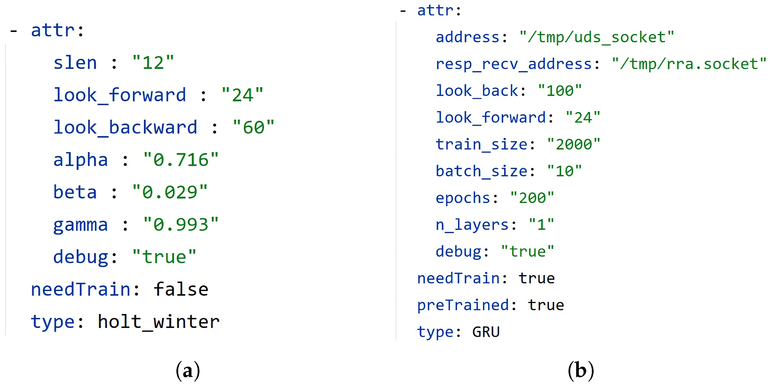
The relevant parameters of the model are defined in the CRD YAML configuration file (Figure 10), and after submitting it to the Kubernetes API Server using the ‘kubectl apply -f’ command, corresponding CRD objects are created in the cluster, enabling predictive scaling functionality.
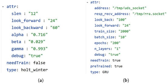
Figure 10.
Model configurations. (a) Holt–Winter model parameter configuration in CRD YAML configuration. (b) GRU model parameter configuration in CRD YAML configuration.
During prediction, the component selects the best available model for the moment and uses it for predictions. Based on the prediction results, it scales resources for the backend service up during peak request periods and scales them down during off-peak times. The Grafana monitoring panel is shown below (Figure 11):
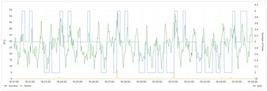
Figure 11.
After the deployment of the scaling component, the monitoring panel for the backend service.
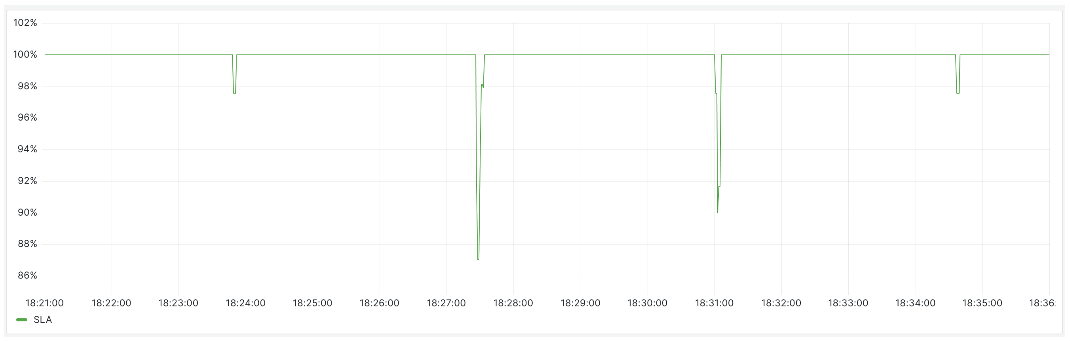
It can be seen from Figure 12 that after the component deployment, the minimum SLA is 87%, and the number of SLA fluctuations has decreased from 24 times in the 15 min before deployment to 4 times in the subsequent 15 min. This indicates a improvement in overall service quality.
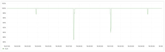
Figure 12.
After the deployment of the scaling component, the SLA status for the backend service.
5. Discussion
We conducted experiments to compare the deployment of the predictive auto-scaling component with the non-deployment scenario, and observed a significant improvement in performance in the cluster in which the component was deployed.
The experimental results reveal that, with the deployment of the predictive auto-scaling Operator, it is effective at acquiring application metrics, predicting based on these metrics, and executing scaling operations. Regarding metric prediction, Table 4 indicates that, when comparing the Holt–Winters algorithm with the GRU, GRU achieves a lower MSE, with a value of 0.01756, whereas the MSE for Holt–Winters is 0.00166. However, in real-time data environments, GRU requires more preparation time. The multi-model management approach in the Operator leverages the strengths of both algorithms, reducing the cold start time of predictive auto-scaling by 1 h and 41 min compared to the start time observed when using only the GRU model, demonstrating an earlier effectiveness of the system.
In terms of application service quality, after deploying the Operator, a noticeable decrease in request errors is observed, with more requests being correctly processed, leading to an 83.3% reduction in the frequency of service-quality fluctuations, as depicted in Figure 8 and Figure 11. In terms of SLA, a comparison between Figure 9 and Figure 12 shows that the minimum SLA of the application has increased from 80.3% to 87%, and after deploying the Operator, the SLA is maintained at 100% for a longer duration.
This system is applicable in cloud-native environments based on Kubernetes. The development model of the Kubernetes Operator allows the system to be directly managed by Kubernetes itself, ensuring reliability. Additionally, the system’s architecture supports the extension of more predictive models, adapting to diverse application scenarios.
6. Conclusions
Scalability is a crucial attribute in cloud environments, aiming to enhance the elasticity and enable more effective management and scaling of resources in the cloud. This study designs and implements a predictive Kubernetes operator that utilizes various time series forecasting algorithms to predict various metrics of monitored services. The experimental results demonstrate that the predictive auto-scaling component helps the system better meet the performance metrics defined in the SLA, validating our initial hypothesis that predictive auto-scaling has a positive impact on service quality in Kubernetes environments.
In this paper, we solely focused on the deployment and integration of algorithms in the experimental environment, and the number of integrated algorithms is limited. Future research can focus on the following directions: further optimization of the integration of predictive algorithms to achieve more efficient and real-time performance prediction and expanding the research scope to a wider range of cloud-native scenarios to examine the adaptability of predictive auto-scaling to different applications and workloads. Finally, another potential topic could be in-depth research on improving training and tuning strategies for predictive models to adapt to constantly changing workload conditions.
Author Contributions
Methodology, S.L.; Software, S.L.; Validation, S.L.; Writing—original draft, S.L.; Writing—review & editing, H.Y.; Supervision, H.Y.; Project administration, H.Y. All authors have read and agreed to the published version of the manuscript.
Funding
This research received no external funding.
Data Availability Statement
Data are contained within the article.
Conflicts of Interest
The authors declare no conflict of interest.
Abbreviations
The following abbreviations are used in this article:
| HPA | Horizontal Pod Autoscaling |
| VPA | Vertical Pod Autoscaling |
| RNN | Recurrent Neural Network |
| GRU | Gated Recurrent Unit |
| LSTM | Long Short-Term Memory |
| CRD | Custom Resource Definitions |
| UDS | Unix Domain Socket |
| TCP | Transmission Control Protocol |
| MSE | Mean Squared Error |
| SLA | Service Level Agreement |
References
- Abeni, L.; Faggioli, D. Using Xen and KVM as real-time hypervisors. J. Syst. Archit. 2020, 106, 101709. [Google Scholar] [CrossRef]
- Malviya, A.; Dwivedi, R.K. A comparative analysis of container orchestration tools in cloud computing. In Proceedings of the 2022 9th International Conference on Computing for Sustainable Global Development (INDIACom), New Delhi, India, 23–25 March 2022; pp. 698–703. [Google Scholar]
- Anderson, C. Docker [software engineering]. IEEE Softw. 2015, 32, 102-c3. [Google Scholar] [CrossRef]
- Pahl, C.; Brogi, A.; Soldani, J.; Jamshidi, P. Cloud container technologies: A state-of-the-art review. IEEE Trans. Cloud Comput. 2017, 7, 677–692. [Google Scholar] [CrossRef]
- Shah, J.; Dubaria, D. Building modern clouds: Using docker, kubernetes and Google cloud platform. In Proceedings of the 2019 IEEE 9th Annual Computing and Communication Workshop and Conference (CCWC), Las Vegas, NV, USA, 7–9 January 2019; pp. 184–189. [Google Scholar]
- Burns, B.; Beda, J.; Hightower, K.; Evenson, L. Kubernetes: Up and Running; O’Reilly Media, Inc.: Newton, MA, USA, 2022. [Google Scholar]
- Nguyen, T.T.; Yeom, Y.J.; Kim, T.; Park, D.H.; Kim, S. Horizontal pod autoscaling in kubernetes for elastic container orchestration. Sensors 2020, 20, 4621. [Google Scholar] [CrossRef] [PubMed]
- Choi, B.; Park, J.; Lee, C.; Han, D. pHPA: A proactive autoscaling framework for microservice chain. In Proceedings of the 5th Asia-Pacific Workshop on Networking (APNet 2021), Shenzhen, China, 24–25 June 2021; pp. 65–71. [Google Scholar]
- Zhao, A.; Huang, Q.; Huang, Y.; Zou, L.; Chen, Z.; Song, J. Research on resource prediction model based on kubernetes container auto-scaling technology. IOP Conf. Ser. Mater. Sci. Eng. 2019, 569, 052092. [Google Scholar] [CrossRef]
- Kan, C. DoCloud: An elastic cloud platform for Web applications based on Docker. In Proceedings of the 2016 18th International Conference on Advanced Communication Technology (ICACT), Pyeongchang, Republic of Korea, 31 January–3 February 2016; pp. 478–483. [Google Scholar]
- Iqbal, W.; Erradi, A.; Abdullah, M.; Mahmood, A. Predictive auto-scaling of multi-tier applications using performance varying cloud resources. IEEE Trans. Cloud Comput. 2019, 10, 595–607. [Google Scholar] [CrossRef]
- Saxena, D.; Singh, A.K. A proactive autoscaling and energy-efficient VM allocation framework using online multi-resource neural network for cloud data center. Neurocomputing 2021, 426, 248–264. [Google Scholar] [CrossRef]
- Xue, S.; Qu, C.; Shi, X.; Liao, C.; Zhu, S.; Tan, X.; Ma, L.; Wang, S.; Wang, S.; Hu, Y.; et al. A Meta Reinforcement Learning Approach for Predictive Autoscaling in the Cloud. In Proceedings of the 28th ACM SIGKDD Conference on Knowledge Discovery and Data Mining, Washington, DC, USA, 14–18 August 2022; pp. 4290–4299. [Google Scholar]
- Haq, M.A. SMOTEDNN: A novel model for air pollution forecasting and AQI classification. Comput. Mater. Contin. 2022, 71, 1403–1425. [Google Scholar]
- Haq, M.A. CDLSTM: A novel model for climate change forecasting. Comput. Mater. Contin. 2022, 71, 2363–2381. [Google Scholar]
- Masini, R.P.; Medeiros, M.C.; Mendes, E.F. Machine learning advances for time series forecasting. J. Econ. Surv. 2023, 37, 76–111. [Google Scholar] [CrossRef]
- Balla, D.; Simon, C.; Maliosz, M. Adaptive scaling of Kubernetes pods. In Proceedings of the NOMS 2020—2020 IEEE/IFIP Network Operations and Management Symposium, Budapest, Hungary, 20–24 April 2020; pp. 1–5. [Google Scholar]
- Knative Pod Autoscaler. Available online: https://www.alibabacloud.com/help/en/ack/ack-managed-and-ack-dedicated/user-guide/enable-automatic-scaling-for-pods-based-on-the-number-of-requests/?spm=a2c63.p38356.0.0.551741bbBm0ZNB (accessed on 10 October 2023).
- Kubernetes Event-Driven Autoscaling. Available online: https://keda.sh/docs/2.12/concepts/#architecture (accessed on 7 December 2023).
- Imdoukh, M.; Ahmad, I.; Alfailakawi, M.G. Machine learning-based auto-scaling for containerized applications. Neural Comput. Appl. 2020, 32, 9745–9760. [Google Scholar] [CrossRef]
- Dang-Quang, N.M.; Yoo, M. Deep learning-based autoscaling using bidirectional long short-term memory for kubernetes. Appl. Sci. 2021, 11, 3835. [Google Scholar] [CrossRef]
- Shim, S.; Dhokariya, A.; Doshi, D.; Upadhye, S.; Patwari, V.; Park, J.Y. Predictive Auto-scaler for Kubernetes Cloud. In Proceedings of the 2023 IEEE International Systems Conference (SysCon), Vancouver, BC, Canada, 17–20 April 2023; pp. 1–8. [Google Scholar]
- Chatfield, C. The Holt-winters forecasting procedure. J. R. Stat. Soc. Ser. 1978, 27, 264–279. [Google Scholar] [CrossRef]
- Cho, K.; Van Merriënboer, B.; Gulcehre, C.; Bahdanau, D.; Bougares, F.; Schwenk, H.; Bengio, Y. Learning phrase representations using RNN encoder-decoder for statistical machine translation. arXiv 2014, arXiv:1406.1078. [Google Scholar]
- Shewalkar, A.; Nyavanandi, D.; Ludwig, S.A. Performance evaluation of deep neural networks applied to speech recognition: RNN, LSTM and GRU. J. Artif. Intell. Soft Comput. Res. 2019, 9, 235–245. [Google Scholar] [CrossRef]
- Kanai, S.; Fujiwara, Y.; Iwamura, S. Preventing gradient explosions in gated recurrent units. In Proceedings of the Advances in Neural Information Processing Systems, Long Beach, CA, USA, 4–9 December 2017; Volume 30. [Google Scholar]
- Brazil, B. Prometheus: Up and Running: Infrastructure and Application Performance Monitoring; O’Reilly Media, Inc.: Newton, MA, USA, 2018. [Google Scholar]


Disclaimer/Publisher’s Note: The statements, opinions and data contained in all publications are solely those of the individual author(s) and contributor(s) and not of MDPI and/or the editor(s). MDPI and/or the editor(s) disclaim responsibility for any injury to people or property resulting from any ideas, methods, instructions or products referred to in the content. |
© 2024 by the authors. Licensee MDPI, Basel, Switzerland. This article is an open access article distributed under the terms and conditions of the Creative Commons Attribution (CC BY) license (https://creativecommons.org/licenses/by/4.0/).