The Validation and Implementation of the Second-Order Adaptive Fuzzy Logic Controller of a Double-Fed Induction Generator in an Oscillating Water Column

Abstract

This article presents a second-order adaptive fuzzy logic controller (SO-AFLC) to improve the performance of a grid-connected double-fed induction generator (DFIG) in an oscillating water column power plant (OWCPP). The proposed SO-AFLC was used to improve the maximum power point tracking (MPPT), DC link voltage stability, and reactive power tracking for the DFIG oscillating water column power plant. The SO-AFLC reduces oscillations, overshooting, and mean square error. The SO-AFLC improved the mean square error by 40.4% in comparison to the adaptive fuzzy logic controller (AFLC) and by 84.9% in comparison to the proportional–integral differential controllers (PIDs). To validate the simulation results, an experimental investigation was performed on the Dspace DS 1104 control board. The SO-AFLC shows a faster response time, reduced undershooting, lower peak overshooting, and very low steady-state error in terms of DC link voltage, rotor speed, and maximum power point tracking. Moreover, the integral absolute error (IAE) index of the oscillating water column turbine was calculated. This index is meant to evaluate the SO-AFLC’s feasibility against the PID and AFLC under the same wave conditions.

1. Introduction

Because traditional fossil fuels are running out, renewable energy supplies will become increasingly popular as alternatives. Our oceans, which represent two thirds of the Earth’s surface, contain tremendous quantities of energy stored in waves, tides, salinity, and other forms. Around 2 TW is the theoretically calculated global ocean wave energy [1,2]. There are several methods to benefit from wave energy. One of these methods is the oscillating water column. An OWC is made up of a chamber that is partially immersed in water. Owing to wave motion, the water inside the chamber oscillates, causing the air flow speed inside the chamber to vary. The change in the air flow speed forces the turbine blades to rotate. The turbine is linked to a DFIG whose stator is directly connected to the grid network, and its rotor is connected to the grid through a rotor-side converter and grid-side converter [3]. Oscillating water column turbines are ideal for a variety of generators, including permanent magnet synchronous generators (PMSGs) and double-fed induction generators (DFIGs). Permanent magnet (PM) machines are still difficult to manufacture due to their high cost and demagnetization at elevated temperatures. Nonetheless, a lot of turbines have DFIGs, which offer some advantages over conventional generators despite their intricate construction [4]. The main advantage of DFIGs are their broad speed range, which is 20–30% higher or lower than synchronous speed. Consequently, the converter can only manage up to 20–30% of the rated power [5,6]. The DFIG’s rotor is connected to the network grid through a rotor-side converter (RSC) and a grid-side converter (GSC). While these converters can improve the overall characteristics of the system [7], they are more expensive than DFIGs due to their use of rare earth materials in their production [8]. The control of a RSC is used to adjust the DFIG in OWCPP at maximum power point tracking by adjusting the flow coefficient [9,10]. Reactive power control is one of the GSC functions used to maintain the unity power factor. For the OWCPP to operate as smoothly as possible, the DC link voltage level is also set to a constant level [10,11,12,13]. Six controllers will be required by the RSC and GSC to carry out these duties. PID controllers are widely used in oscillating water systems because of their many advantages, which include their wide stability margins, low adjustment parameters, system durability, and simple construction. Additionally, many methods for designing the PIDs used in the grid-integrated OWCPP control strategy have been proposed, including the Ziegler–Nichols (ZN) algorithm [14,15] and particle swarm optimization (PSO) [16]. The most effective one is the self-adaptive global harmony search (SGHS) algorithm [17]. Among the many benefits associate with PID controllers are their broad stability range, robustness, straightforward design, and the ease of choosing of gains. The sensitivity of the PID controllers to the nonlinearity and variable changes in the system causes the system to become unstable [3].

AFLCs for PI are very promising controllers that solve the problem of conventional PI and PIDs. The volatility of the integrated control system is increased using the adaptive fuzzy logic controller. AFLCs are designed by combining fuzzy logic controllers and PI [18,19,20]. AFLCs have inherent advantages, such as how they handle uncertainty in systems, their model-free methodology, and their simple architectures. AFLCs also have the potential to perform better in terms of power tracking compared to other methods such as fuzzy logic controllers and conventional PI [18]. However, in terms of dynamic response in the cascading control system, currently, AFLCs experience certain limitations [21]. Consequently, this paper proposes the enhancement of the AFLC presented in [18,19,20] by including a second-order sliding mode in the AFLC [22,23] to circumvent these drawbacks. While the AFLC operates at the steady-state stage to minimize chatter in response, the second-order sliding mode functions in the transient stage to provide a rapid dynamic response and enhance the stability of the system during the transient state. As a result, the SO-AFLC does not have longer execution times or more memory. The results of using SO-AFLCs included a rapid response time, fast rate of convergence, minimal undershooting, less overshooting, and minimal steady-state error concerning DC link voltage, rotor speed, and maximum power point tracking compared with those implemented using a PI and/or AFLC.

To the extent of the knowledge we have, the SO-AFLC has not addressed in the literature in the context of clean energy resources. The critical contributions of this paper are as follows:

• Investigating the robustness of using SO-AFLCs, which are used in rotor-side converters and grid-side converters.
• Validating the OWCPP performance of SO-AFLCs and comparing it to that of the SGHS-PID methodology and a AFLC.
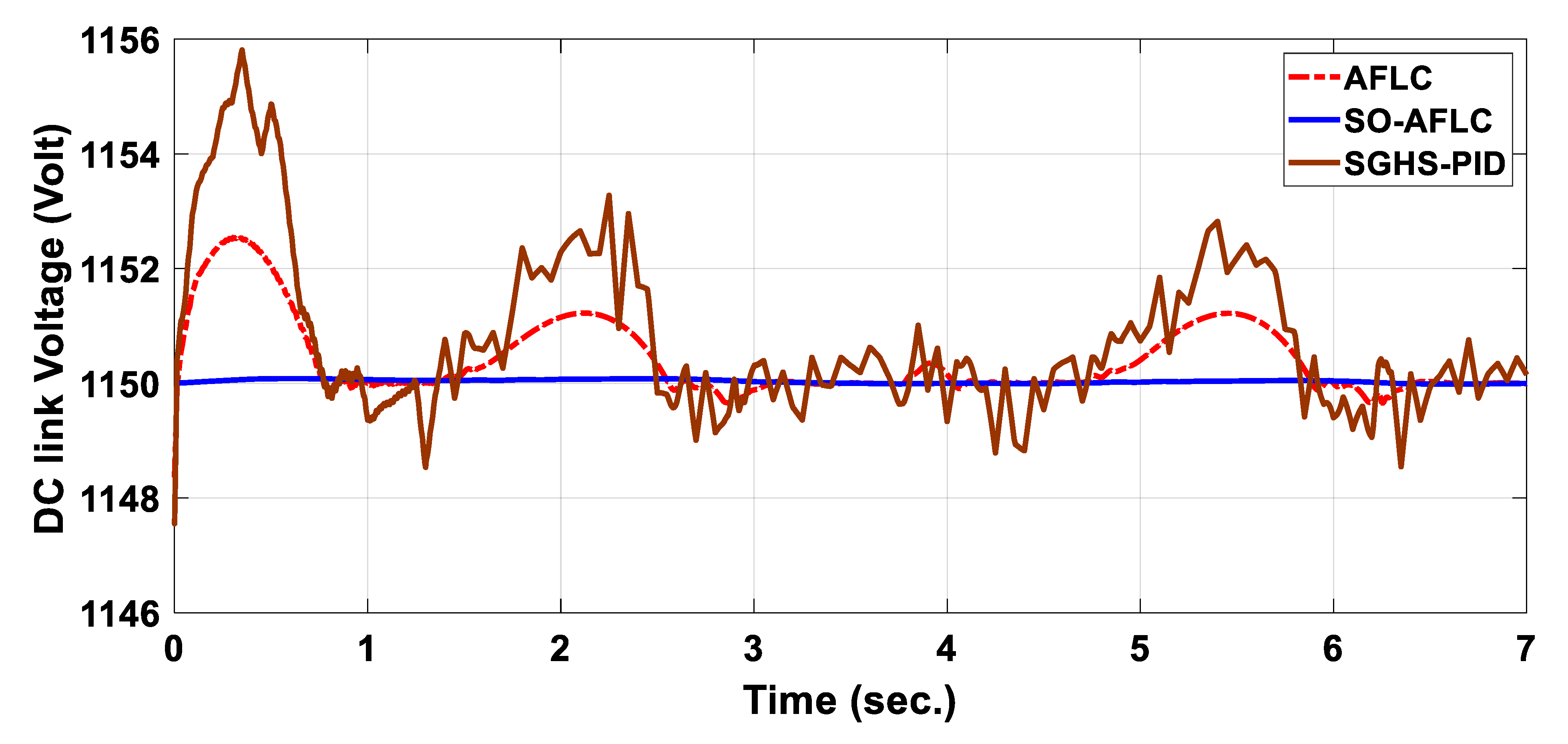
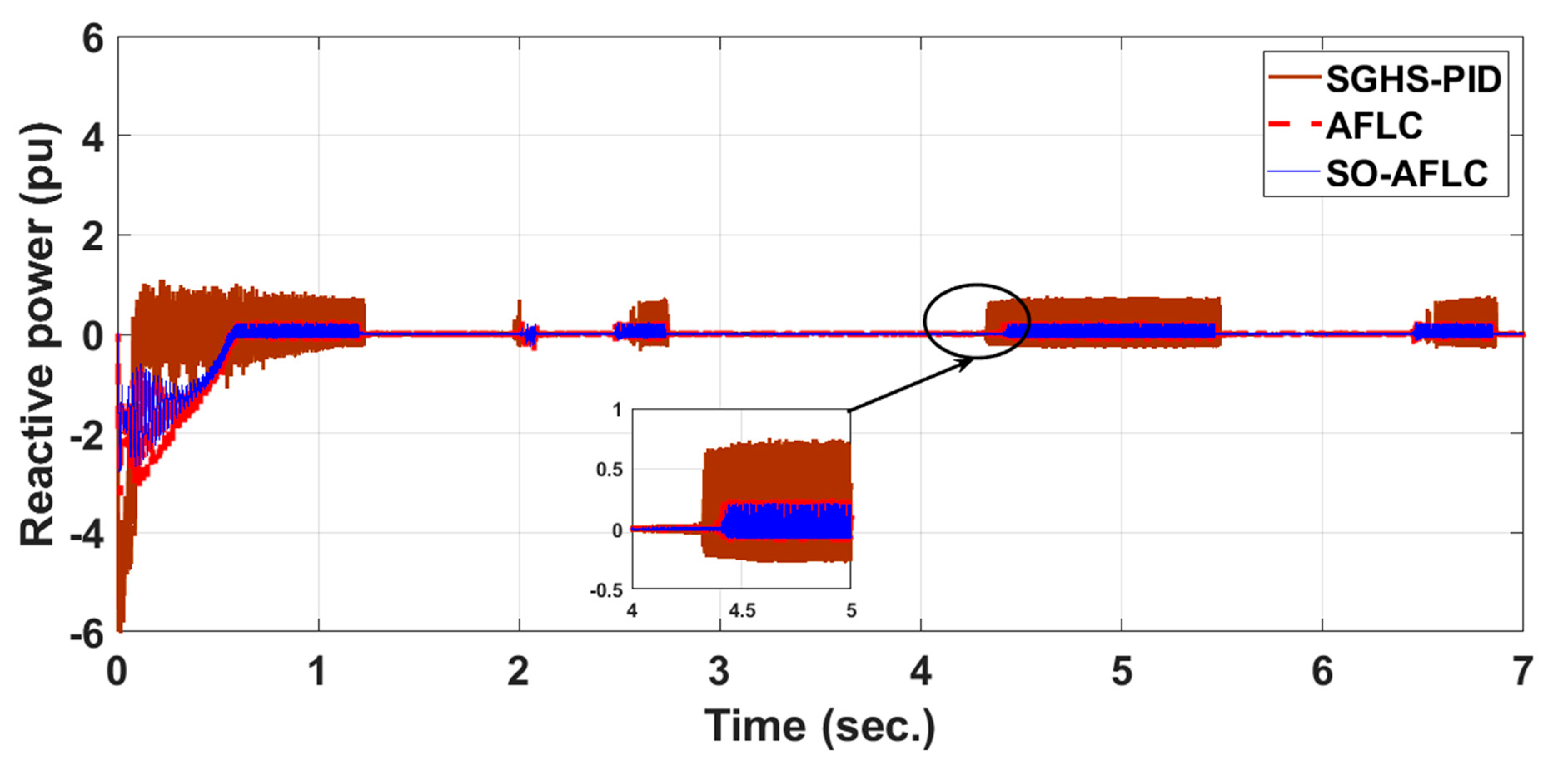
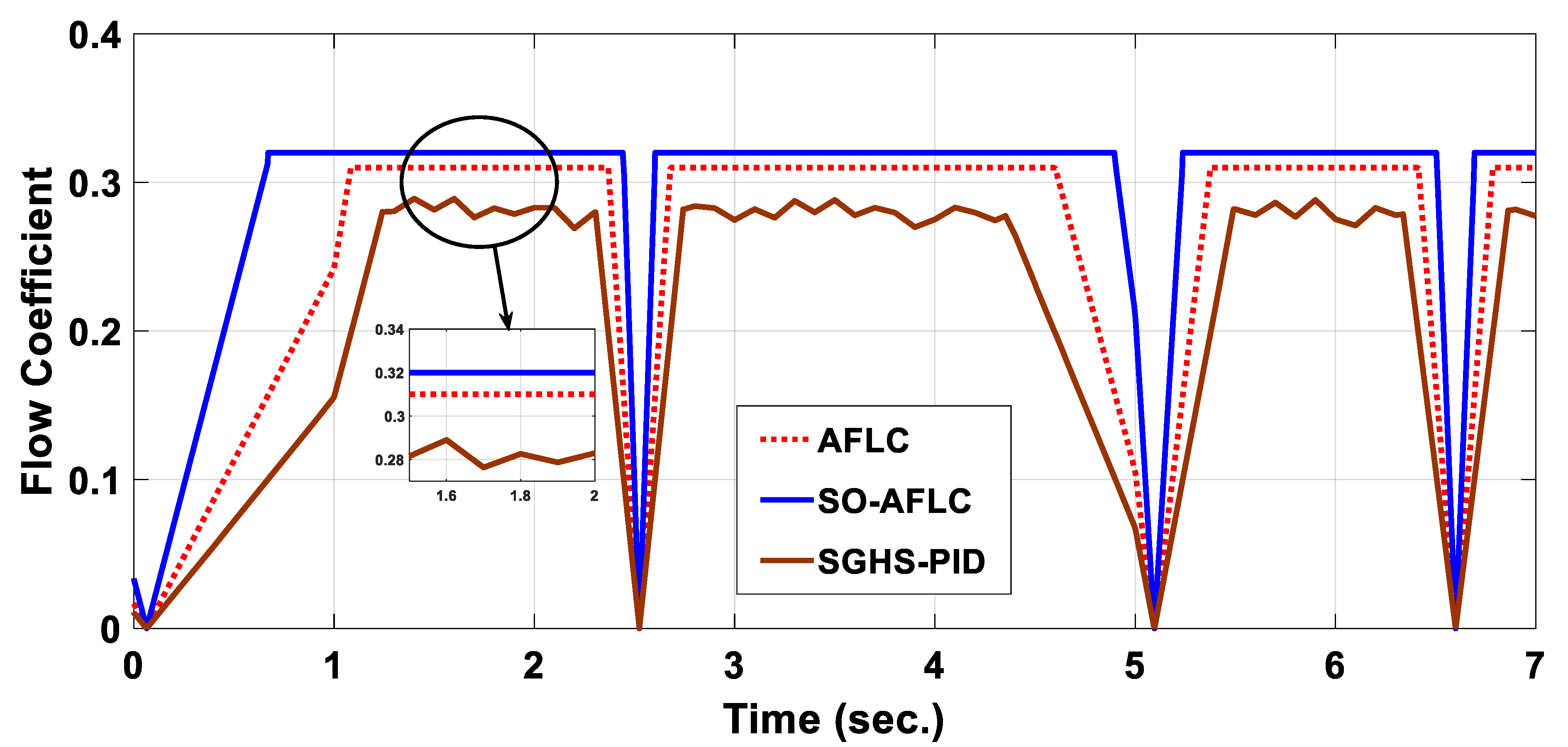
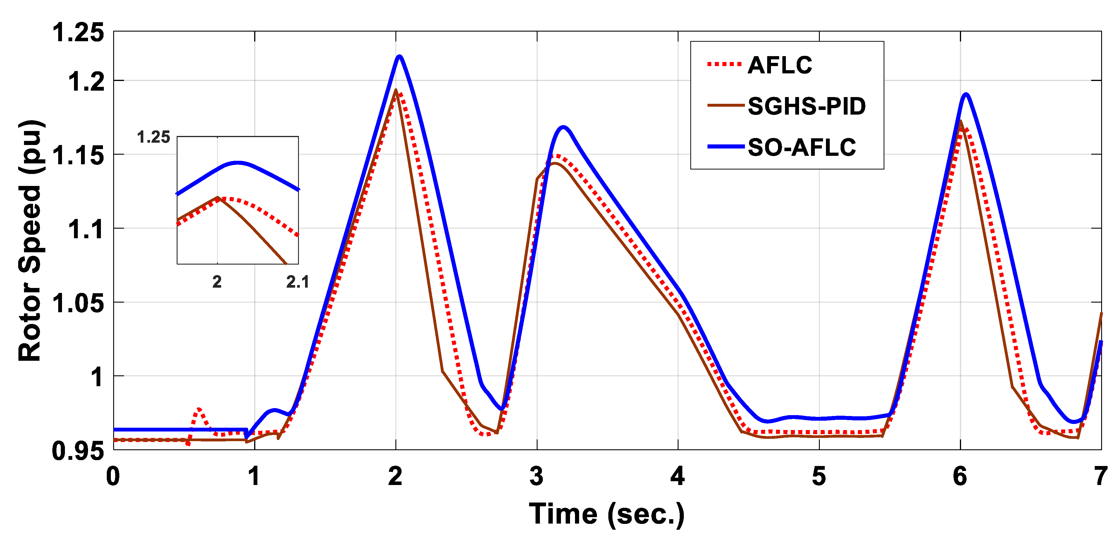
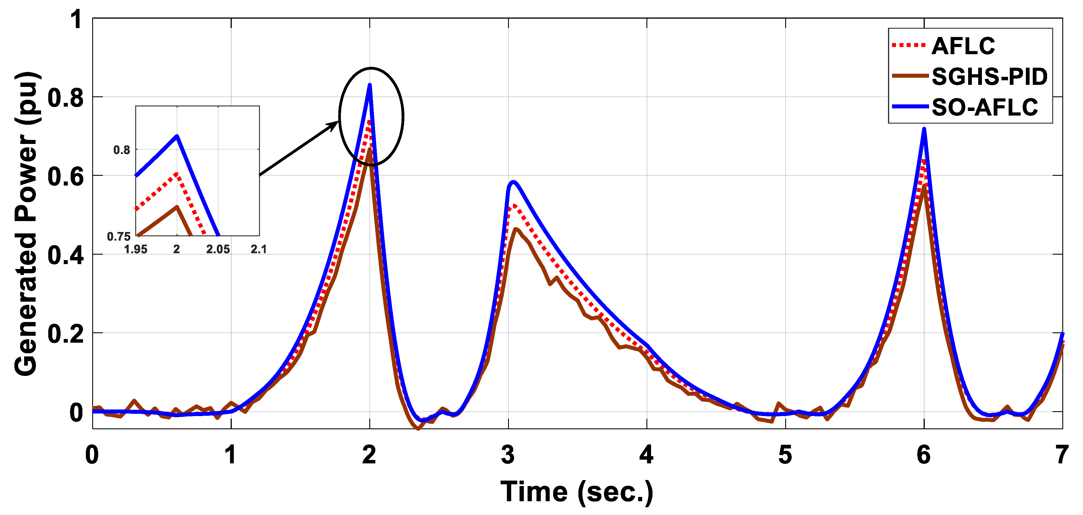
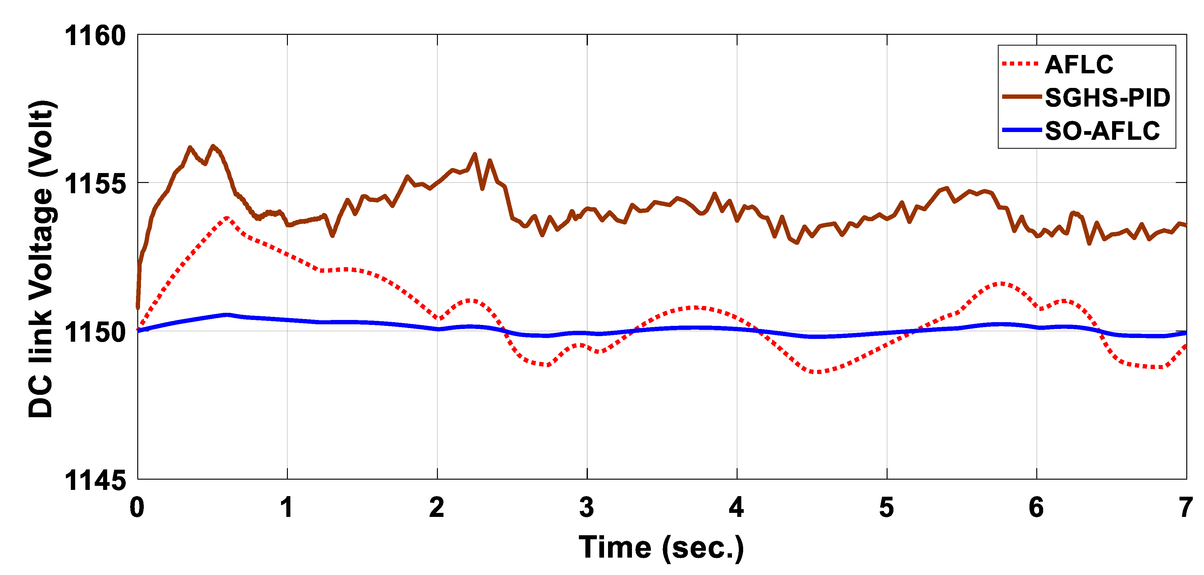
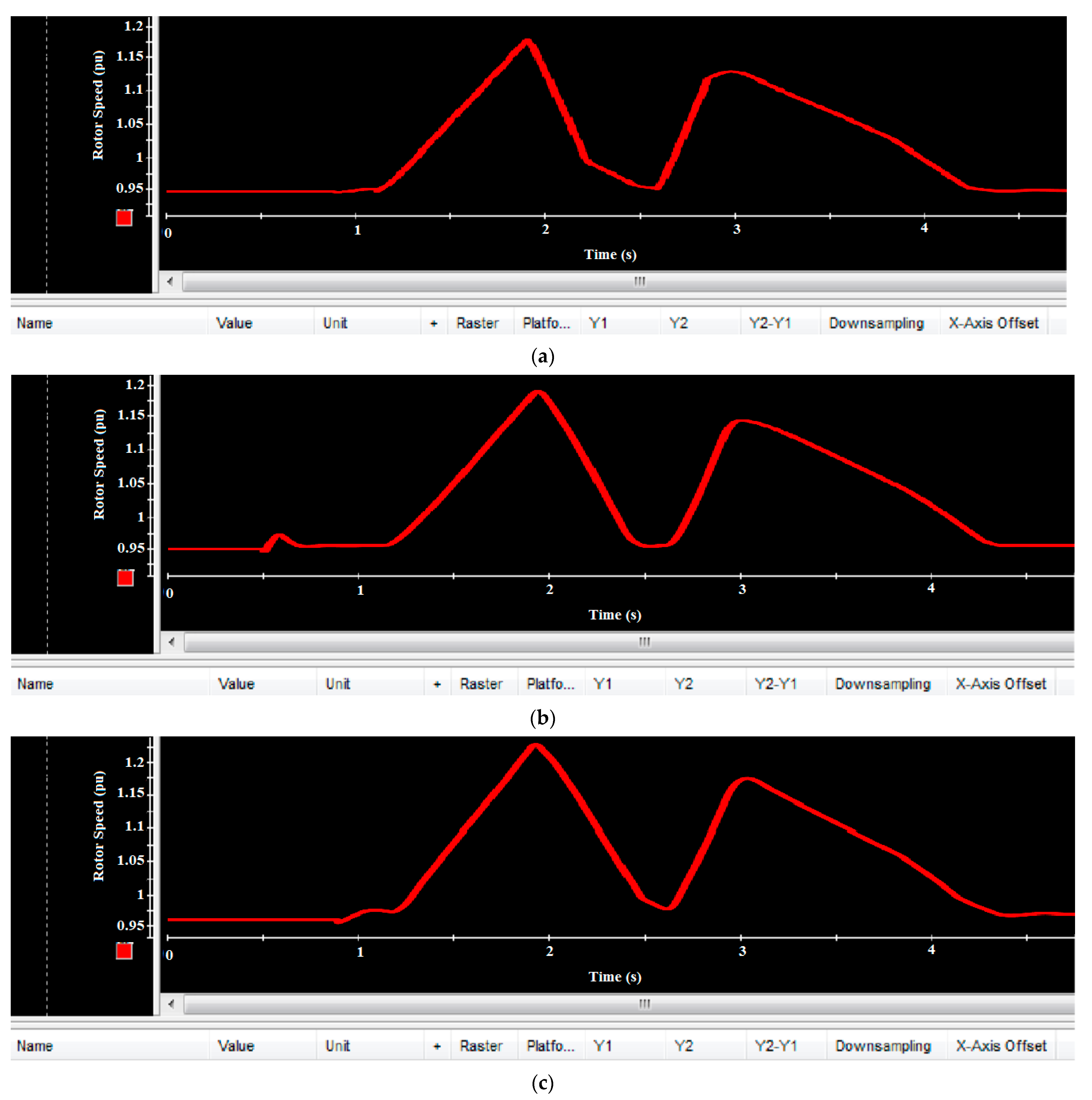
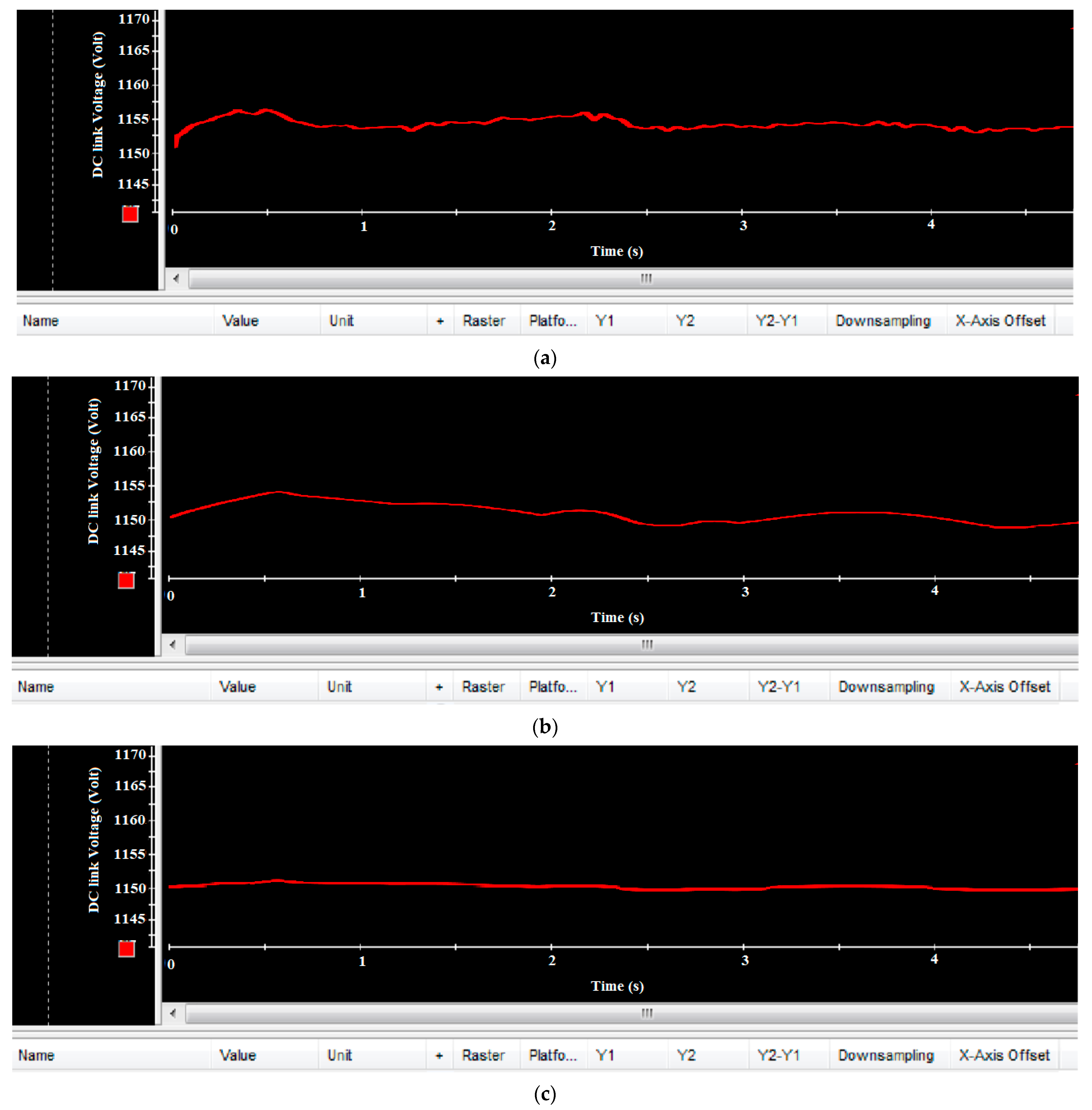
• Improving the power tracking, rotor speed-tracing, and DC link voltage responses.
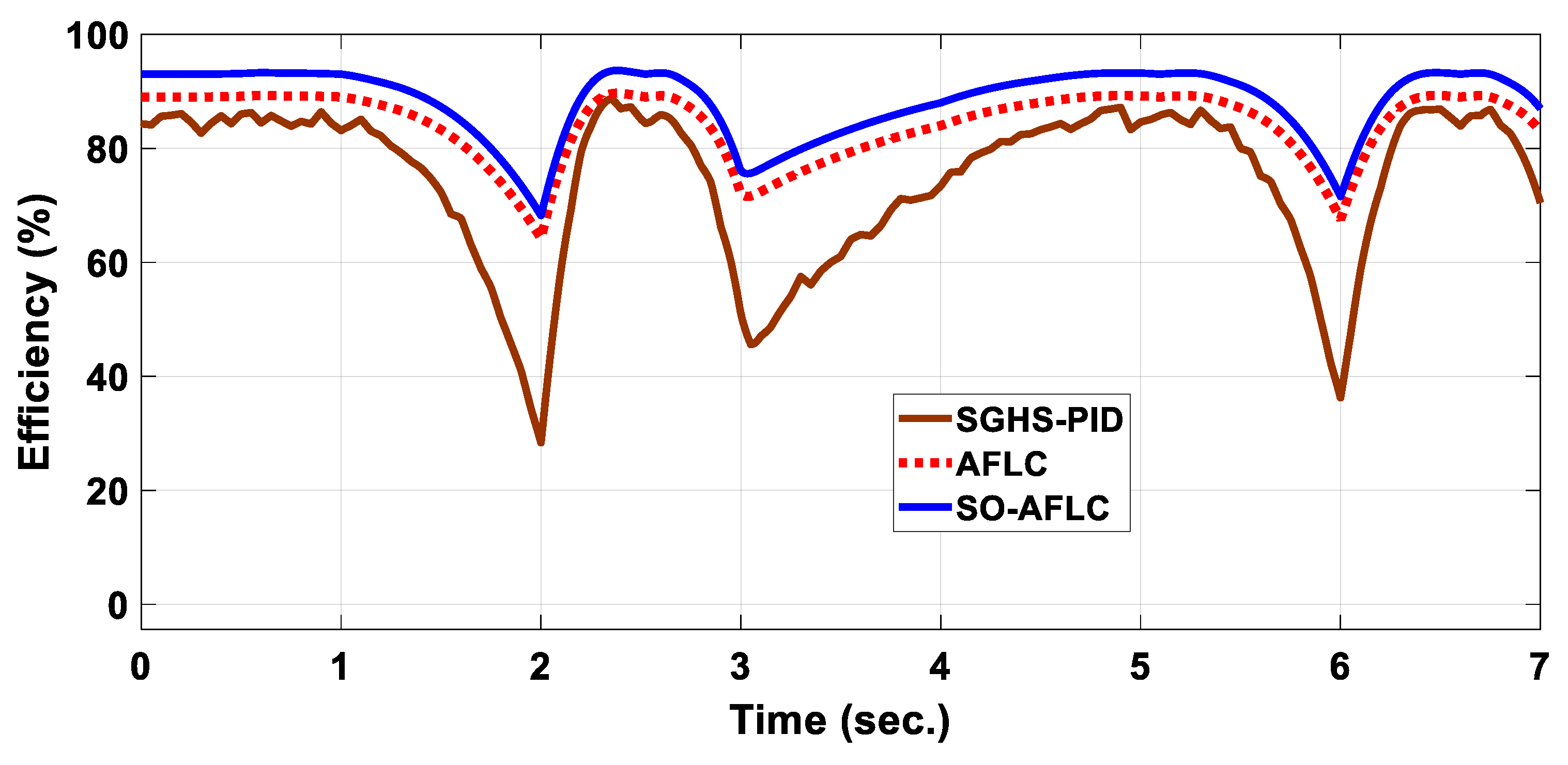
• To demonstrate the SO-AFLC methodology’s feasibility using conventional methods, an evaluation index (IAE) is presented under identical wave conditions.
• The validation of the simulation results for the SO-AFLC methodology by evaluating the proposed model using a real-time interface, DSP1104.

The rest of this article is structured as follows: The article’s introduction and an overview of the existing literature are presented in Section 1. The model configuration for a grid-connected OWCPP is covered in Section 2. The simulation results are discussed in Section 3. The hardware setup for the experiment is covered in Section 4. The experimental results derived from utilizing the DS 1104 are discussed in Section 5. Section 6 concludes the article by presenting this study’s findings and notes on future steps.

2. The Configuration of an Oscillating Water Column Power Plant

The OWC is one of the configurations that transforms wave power into electricity. Figure 1 shows a schematic diagram of the entire OWC power plant. In this configuration, an encoder is used to obtain the turbine speed, which provides the value of $\omega$. Three AFLCs are employed in the RSC to improve the rotor speed and power tracking. Another three AFLCS are used in the GSC to enhance the DC link voltage for more efficient operation and to improve the power factor of the machine. The error of AFLC1, which is also used as a speed regulator, is calculated from the measured values of $\omega$ and the optimum airflow rate generator (OARG) using the chamber pressure to adjust the operation of the generator at the maximum power point.

2.1. Mechanical Model of OWC Turbine

The air inside the chamber oscillates because of the change in the height of the waves, changing the air pressure, and the kinetic energy needed to spin the turbine. As is the case in wind turbine generator (WTG) models, the OWC turbine generator can convert the air flow inside the chamber into electricity. The power produced ($p_{in}$) by the OWC turbine can be estimated using Equation (1) [24].

$$p_{in }=\left(dP+\frac{\rho v_x^2}{2}\right)v_{x}a$$

(1)

When the waves rise in the chamber, the interior air pressure ($dP$) rises; conversely, when the water recedes, the pressure is released, causing changes in the speed and direction of the air inside the chamber. Wells turbines always rotate in the same direction, yet they can move in a different direction from the direction of the airflow [25]. The following formula establishes a mathematical model of a wells turbine [26,27]:

$$dP=C_a{k}_t\frac{1}{a}\left[v_x^2+{\left(r\omega \right)}^2\right]$$

(2)

The turbine torque can be defined by Equations (3) and (4).

$$T_t=C_t{k}_{t}r\left[v_x^2+{\left(r\omega \right)}^2\right]$$

(3)

$$T_t=\frac{C_{t}ra}{C_a}dP$$

(4)

The turbine constant can be estimated using Formula (5); the flow coefficient can be estimated using Equation (6).

$$k_t=\rho bn\frac{1}{2}$$

(5)

$$\phi =\frac{v_x}{r\omega }$$

(6)

$$q=v_{x}a$$

(7)

The first-order coupling equation between the OWC turbine and DFIG is illustrated in Equation (8) [22].

$$J\dot{\omega }+B\omega =T_t-\gamma T_e$$

(8)

The relation between the torque coefficient and flow coefficient is illustrated in Figure 2. To accomplish maximum power point tracking, the oscillating water column turbine needs to run at the torque coefficient’s optimal value, which should match the optimal flow coefficient. The diagram shows that the optimum power and torque flow coefficient ${\phi }_{opt}$ is approximately 0.321. This point is defined as the point of stalling where the angle between axial velocity and the tangential velocity reaches around 14⁰. The rotational speed at MPPT is defined by Equation (9).

$${\omega }^{*}=\frac{v_x}{r.{\phi }_{opt}}$$

(9)

2.2. DFIG Modelling

As shown in Figure 3, the double-fed induction generator can be mimicked in a q-d reference frame [28,29].

The voltage ($V_{ds},V_{qs}$) of the stator can be described as follows:

$$V_{ds}=R_s{i}_{ds}-{\omega }_s{\lambda }_{qs}+\frac{d{\lambda }_{ds}}{dt}$$

(10)

$$V_{qs}=R_s{i}_{qs}+{\omega }_s{\lambda }_{ds}+\frac{d{\lambda }_{qs}}{dt}$$

(11)

The voltage ($V_{dr},V_{qr}$) of the rotor can be formulated as follows:

$$V_{dr}=R_r{i}_{dr}-s {\omega }_s{\lambda }_{qr}+\frac{d{\lambda }_{dr}}{dt}$$

(12)

$$V_{qr}=R_r{i}_{qr}+s {\omega }_s{\lambda }_{dr}+\frac{d{\lambda }_{qr}}{dt}$$

(13)

The linkage fluxes of both stators (${\lambda }_{ds},{\lambda }_{qs}$) and the rotor (${\lambda }_{dr},{\lambda }_{qr}$) are written as follows:

$${\lambda }_{ds}=L_{ls}{i}_{ds}+L_m{i}_{dr}$$

(14)

$${\lambda }_{qs}={L_{ls}}_s{i}_{qs}+L_m{i}_{qr}$$

(15)

$${\lambda }_{dr}=L_{lr}{i}_{dr}+L_m{i}_{ds}$$

(16)

$${\lambda }_{qr}=L_{lr}{i}_{qr}+L_m{i}_{qs}$$

(17)

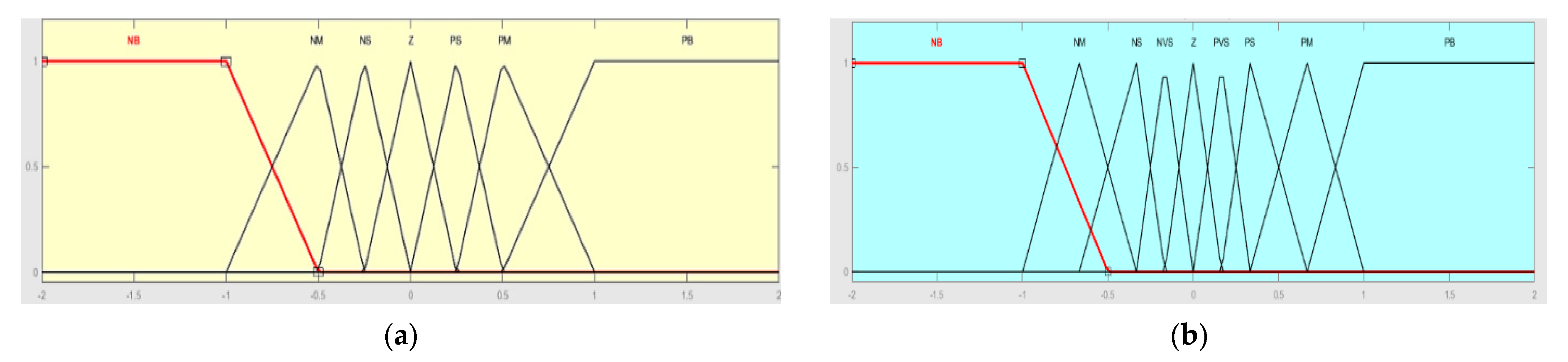
2.3. Adaptive Fuzzy Logic Controller

Adaptive fuzzy logic controllers have shown better performances than other controllers in air-turning turbines [18,19,21]. An AFLC for PI is illustrated in Figure 4. An AFLC consists of a fuzzy logic controller (FLC) and a proportional-integral (PI) controller [30]. The PI control input is adjusted by the FLC. The RSC control part requires three regulators to obtain the maximum power from the OWCPP. The GSC control part needs three different regulators to adjust the DC link voltage between RSC and GSC to obtain the maximum efficient operation from this system; also, it is used for reactive power tracking. All parameters ($K_{Po}$, ${ K}_{do}$, ${ K}_o$, ${ K}_P,$ and $K_i$) are modified for all six controllers to obtain the minimal integral square error (ISE). Increasing membership causes an accurate and high-quality fuzzy system. The membership functions for both inputs and outputs are shown in Figure 5. The memberships are formulated as positive medium (PM), positive big (PB), negative big (NB), negative medium (NM), positive small (PS), zero (Z), and negative small (NS), as illustrated in Figure 5 [31]. The triangle membership functions (MFs) with overlapping on (NB) and (PB) have demonstrated the ability to introduce output/input fuzzy sets with the best accuracy and a tolerable computational cost [32,33]. This restricts the number of firing rules in a two-input FLC to a maximum of four, independent of the quantity of fuzzy sets applied to each input variable. In an unconstrained situation, increasing the number of fuzzy sets per input variable increases the number of rules firing at once, since each FLC input is fuzzified into a growing number of fuzzy sets, each of which depends on the number of fuzzy sets overlapping each other [33].

Table 1. AFLC rules.

e	PS	PM	PB	Z	NS	NM	NB
Δe
NB	NS	NVS	Z	NM	NB	NB	NB
NM	NVS	Z	PVS	NS	NM	NB	NB
NS	Z	PVS	PS	NVS	NS	NM	NB
Z	PVS	PS	PM	Z	NVS	NS	NM
PS	PS	PM	PB	PVS	Z	NVS	NS
PM	PM	PB	PB	PS	PVS	Z	NVS
PB	PB	PB	PB	PM	PS	PVS	Z

shows the rules of the AFLC.

2.4. Second-Order Adaptive Fuzzy Logic Controller

This controller can also be called a second-order adaptive sliding mode controller (SO-ASMC). It consists of two controllers: the second-order sliding mode controller and AFLC. Then, the SO-AFLC combines the advantages of both regulators. Figure 6 shows a schematic diagram for the SO-AFLC. The second-order sliding mode functions when the system is in a transient state, providing a rapid dynamic response and enhancing the stability of the system. The operation of this proposed control strategy is divided into two stages. In the first stage, the sliding surface (SS) is established after the control rule is designed in order to guide the regulator to track the reference abruptly [25,26,27,28,29]. The second-order sliding mode controller operates to provide a rapid dynamic response and enhance the stability of the system during the system’s transient state [34]. The SS is computed by taking the second derivatives of the error. In the second stage, the adaptive fuzzy logic controller serves to minimize the chatter in the responses. In the second-order sliding mode, the derivatives and the error are always pointed at the SS. Takagi–Sugeno optimization is used to achieve the optimum gains of the controller [35]. The mathematical equation for the SS is listed below:

$$SS=K_L\ddot{e}\left(t\right)+\zeta \left(t\right)$$

(18)

In structures that employ PWM to prevent oscillation and chattering problems, Equation (19) is employed.

$$Desired Output=-\mathsf{\Lambda }\mathrm{s}\mathrm{a}\mathrm{t}\left(\mathrm{S}\mathrm{S},\mathsf{\varrho }\right)=-\mathsf{\Lambda }\left[\frac{SS}{\left|SS\right|+\varrho }\right]$$

(19)

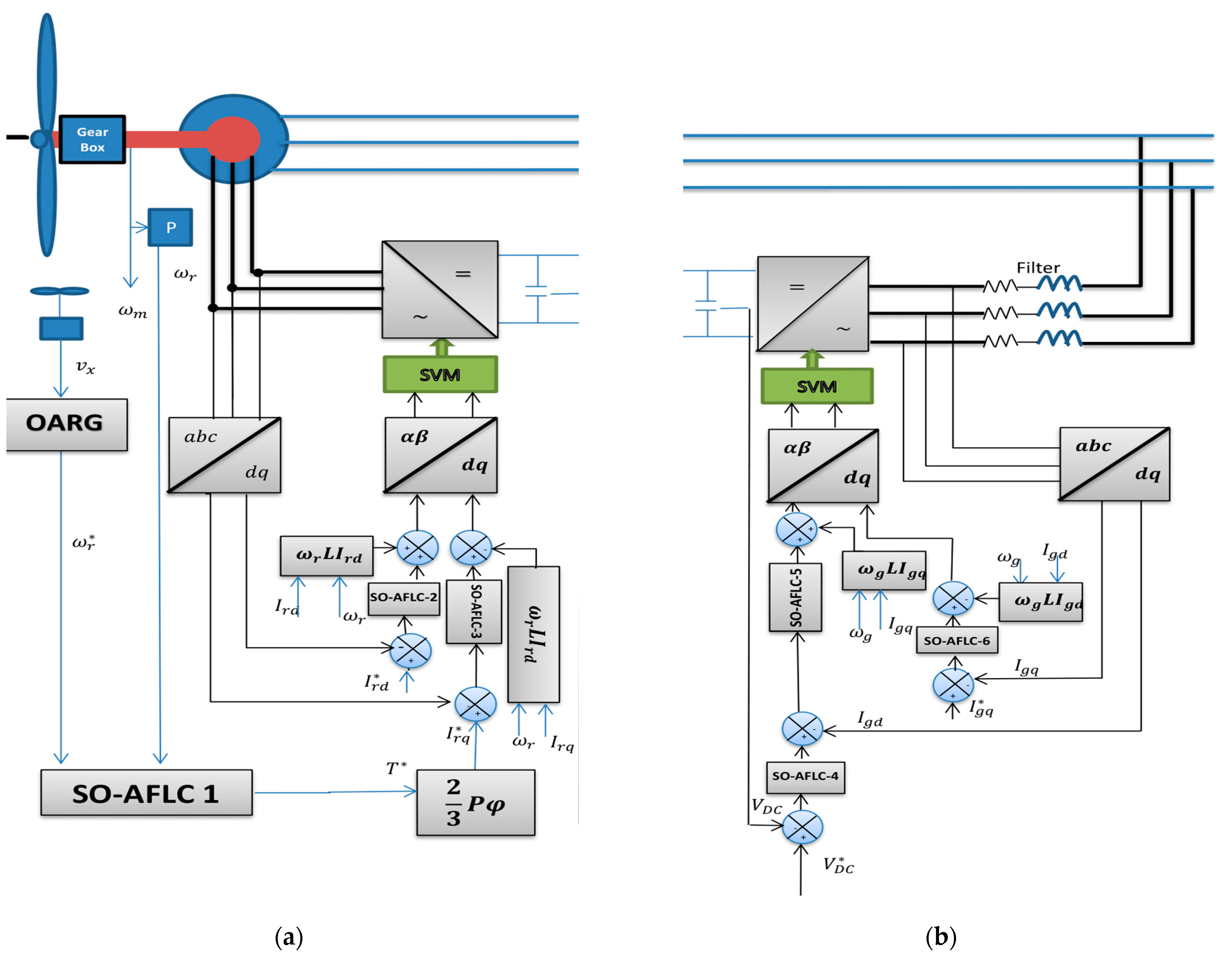
2.5. Grid-Side Converter and Rotor-Side Converter

The Rotor of the DFIG is connected to the grid network through a RSC and GSC. The RSC is illustrated in Figure 7a. The main purpose of a RSC is to establish the MPPT by forcing the DFIG to operate at the optimum flow coefficient ${\phi }_{opt}$ using SO-AFLC 1, SO-AFLC 2, and SO-AFLC 3. If the speed of the air flow inside the chamber changes, the turbine rotor speed will be readjusted in a way that serves to adjust to the change in airflow speed. GSC is illustrated in Figure 7b. The main purpose of the GSC is to adjust the DC link voltage using SO-AFLC 4 and SO-AFLC 5 and the power factor using SO-AFLC 6. The DC link voltage between the RSC and GSC is adjusted at a fixed value for the most efficient operation of the DFIG. The power factor is adjusted to unity by controlling the reactive power to ensure that it is set to zero.

3. Simulation Results

We simulated the use of SO-AFLCs for grid-connected oscillating water columns using Matlab/Simulink 2023a. SO-AFLCs are used for both RSC control and GSC control to achieve maximum power point tracking, reactive power control, and DC link voltage tracking under periodic wave change and random wave change. The DFIG parameters are illustrated in

Table 2. DFIG parameters.

$\mathbf{Nominal} \mathbf{Power} \mathbf{\left(}{\mathit{P}}_{\mathit{n}\mathit{o}\mathit{m}}\mathbf{\right)}$	Frequency (f)	$\mathbf{Voltage} \mathbf{\left(}{\mathit{V}}_{\mathit{n}\mathit{o}\mathit{m}}\mathbf{\right)}$	Rotor Resistance $\mathbf{\left(}{\mathit{R}}_{\mathit{r}}\mathbf{\right)}$	Stator $\mathbf{Resistance} \mathbf{\left(}{\mathit{R}}_{\mathit{s}}\mathbf{\right)}$	Stator Leakage Inductance $\mathbf{\left(}{\mathit{L}}_{\mathit{l}\mathit{s}}\mathbf{\right)}$	Rotor Leakage Inductance $\mathbf{\left(}{\mathit{L}}_{\mathit{l}\mathit{r}}\mathbf{\right)}$	Magnetization Inductance $\mathbf{\left(}{\mathit{L}}_{\mathit{m}}\mathbf{\right)}$	No. of Pair Poles
$1650 \mathrm{k}\mathrm{w}$	50 Hz	575 V	0.0050 pu	0.0071 pu	0.171 pu	0.1560 pu	2.9 pu	3

. The optimum gains for six controllers are described in

Table 3. Controller parameters.

	PID			AFLC					SO-AFLC
	${\mathit{K}}_{\mathit{p}}$	${\mathit{K}}_{\mathit{i}}$	${\mathit{K}}_{\mathit{d}}$	${\mathit{K}}_0$	${\mathit{K}}_{\mathit{p}\mathit{o}}$	${\mathit{K}}_{\mathit{d}\mathit{o}}$	${\mathit{K}}_{\mathit{p}}$	${\mathit{K}}_{\mathit{i}}$	${\mathit{K}}_0$	${\mathit{K}}_{\mathit{p}\mathit{o}}$	${\mathit{K}}_{\mathit{d}\mathit{o}}$	${\mathit{K}}_{\mathit{p}}$	${\mathit{K}}_{\mathit{i}}$	${\mathit{K}}_{\mathit{L}}$
Controller 1	23.64	14.775	8.755	0.1563	10.759	4.589	9.756	4.659	2.538	14.189	6.698	10.268	5.272	3.3
Controller 2	4.185	1.581	0.239	2.258	5.236	1.549	5.214	1.248	3.689	5.869	1.869	7.456	2.528	1.8
Controller 3	6.984	3.91	1.235	0.312	1.688	2.516	8.345	0.2789	0.254	1.007	3.681	9.355	2.6029	1.9
Controller 4	5.06	1.628	0.853	0.9815	8.146	0.2789	1.6345	0.544	1.003	8.023	0.3892	1.7455	0.714	1.6
Controller 5	0.89	2.013	1.023	1.246	0.177	5.8721	0.0023	6.234	1.756	0.225	7.78	0.35	9.005	1.14
Controller 6	3.287	1.256	0.028	2.4902	8.012	0.0154	6.567	0.002	3.523	8.443	0.254	8.546	0.0001	2.002

. The PI gains ($K_p$ and $K_i$) were optimized using the self-adaptive global harmony search (SGHS) algorithm [17].

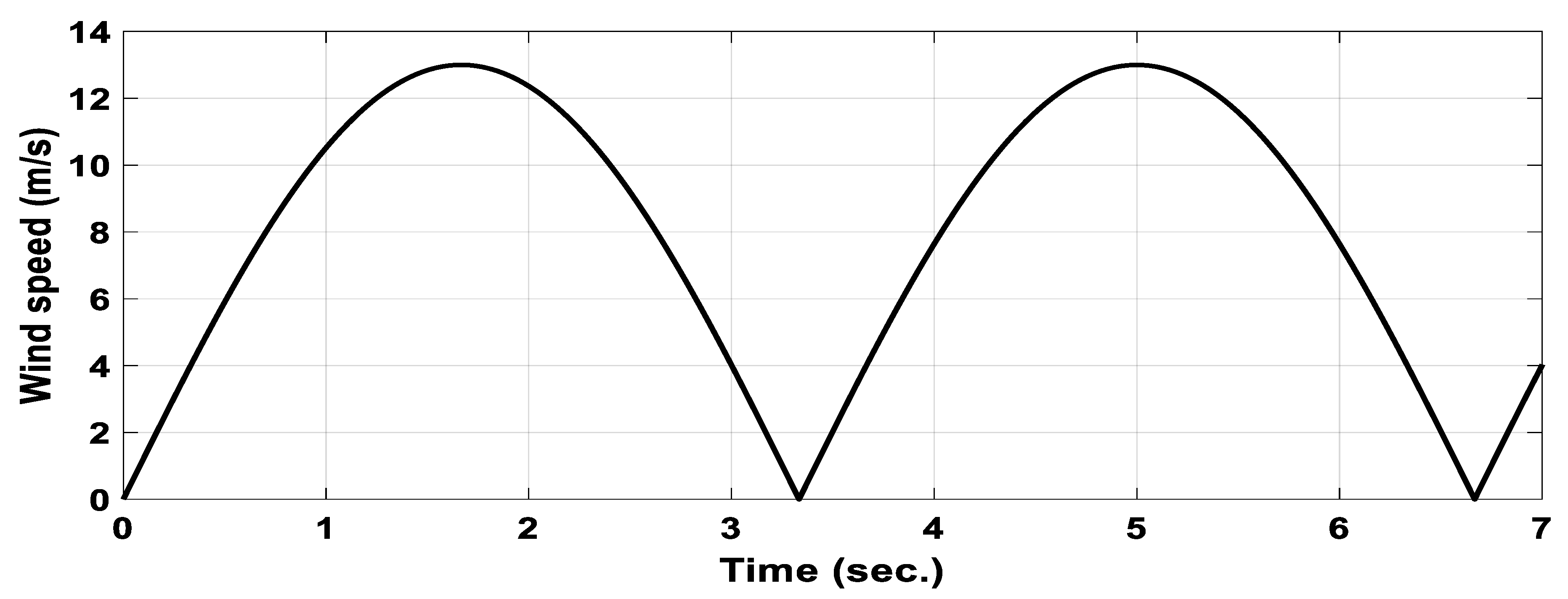
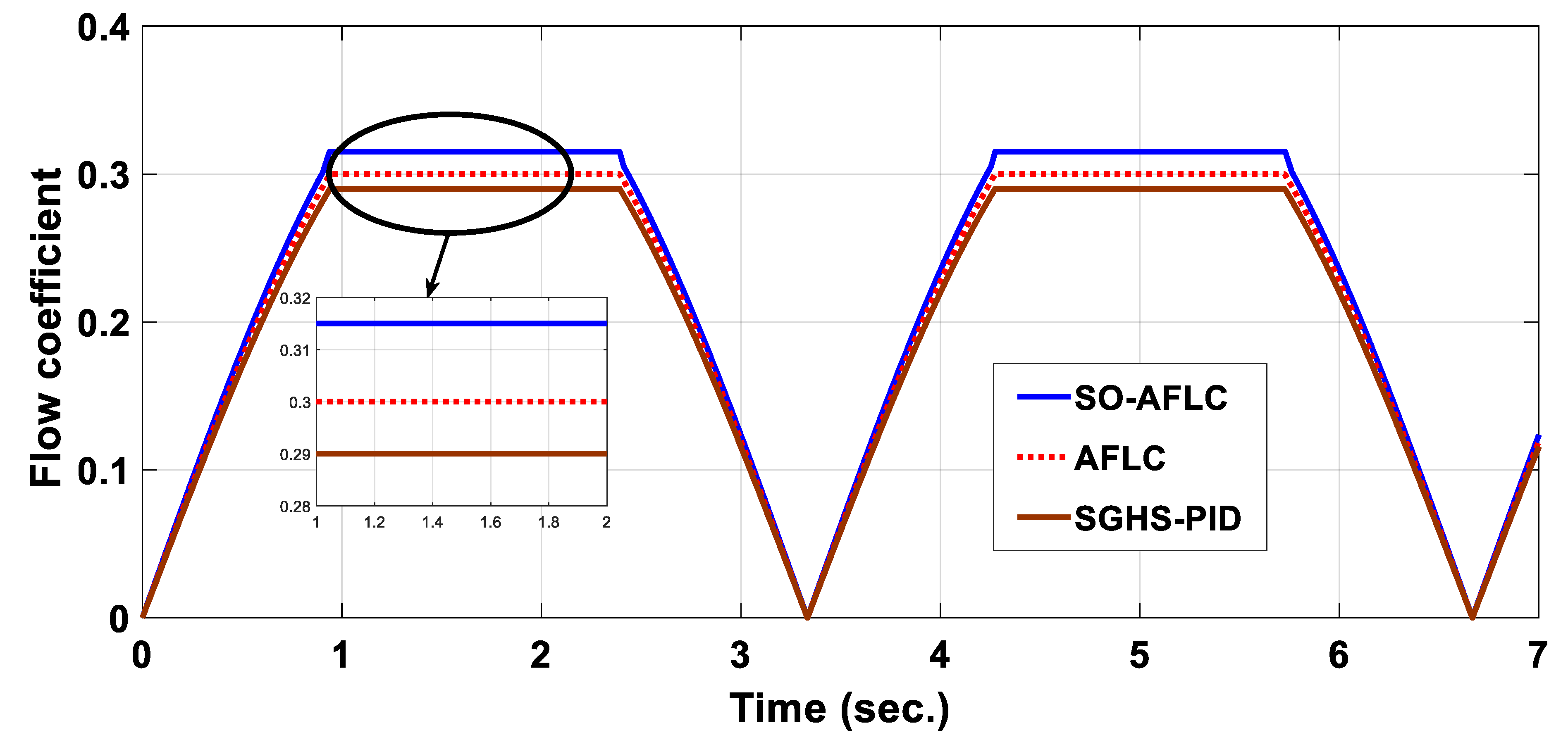
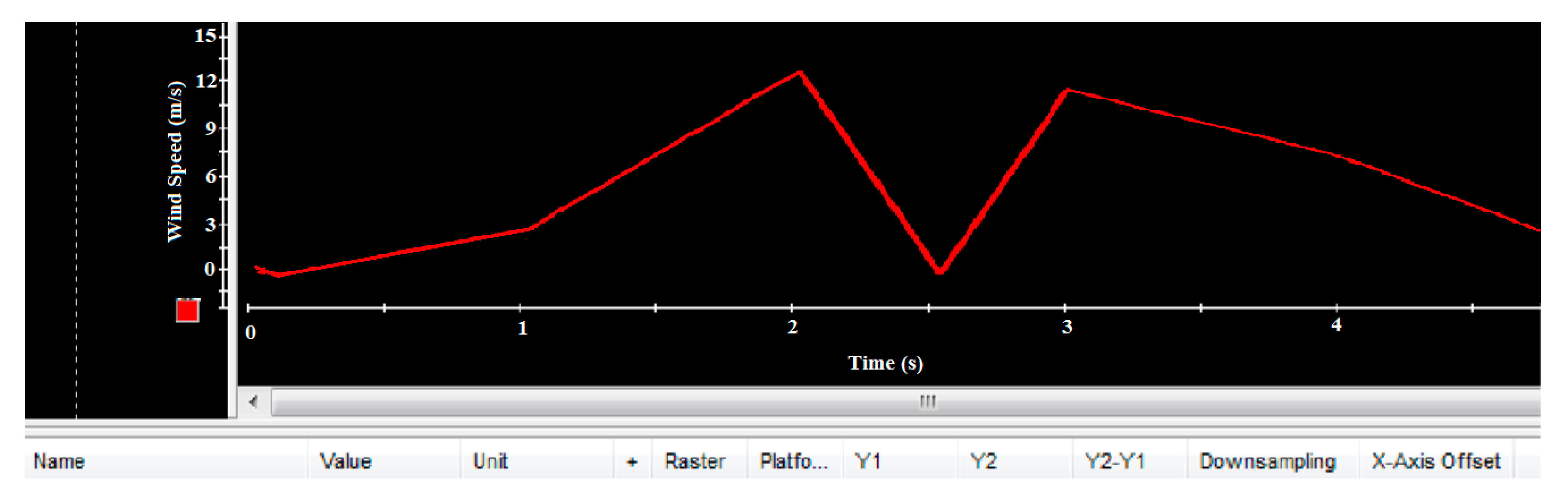
3.1. Case I: Periodic Wave Change

Case I centres around the effect of SO-AFLC on DFIG in a grid-tied OWCPP under periodic sinusoidal wave change [36]. The air flow inside the chamber is shown in Figure 8. The flow coefficient grid-tied OWCPP is illustrated in Figure 9. In comparison to the PID, both the AFLC and SO-AFLC offered quick responses, with the SO-AFLC having a slight edge. Moreover, the SO-AFLC adjusted the flow coefficient to 0.317 with the lowest steady-state error from the threshold of 0.321. The AFLC had a steady-state value of 0.3012. The SGHS-PID had a steady-state value of 0.291. The DFIG’s rotating speed is illustrated in Figure 10. Better speed tracking can be achieved by both the AFLC and SO-AFLC compared to the PID, with a little improvement for the SO-AFLC being observed. Between t = 1.95 s and t = 2.1 s, the SO-AFLC responded faster than the PID and AFLC. The SO-AFLC outperformed the PID and AFLC in terms of rotational speed tracking by 80.61% and 22.3%, respectively. The mechanical power produced by the oscillating turbine is shown in Figure 11. At the peak of air flow speed, the SO-AFLC generates the highest power possible with the best power tracking. The DC voltage between the GSC and RSC is displayed in Figure 12. In comparison to the AFLC and PID, the SO-AFLC reduced the steady-state error in the DC voltage by 1.42 V and 2.83 V, respectively. In Figure 13, the reactive power value is set to zero in order to maintain the unity power factor. Compared to the PID, the SO-AFLC and AFLC both have the lowest error and the best monitoring of reactive power. In the SO-AFLC, errors were slightly less frequent than in the AFLC.

3.2. Case II: Random Wave Change

Under random wave change, the DFIG oscillating water column power plant is investigated using the SO-AFLC. The air flow inside the chamber is shown in Figure 14. Figure 15 shows the flow coefficient of the grid-tied OWCPP. Both the SO-AFLC and AFLC introduced a quick response compared to the PID, with the SO-AFLC having a slight edge. Moreover, the SO-AFLC adjusted the flow coefficient to 0.32 with the lowest steady-state error from the threshold of 0.321. The AFLC had a steady-state value of 0.312. The SGHS-PID had a steady-state value of 0.283. Figure 16 illustrates the DFIG’s rotational speed. Both the AFLC and SO-AFLC had superior speed control compared to the PID, with a slight improvement for the SO-AFLC being observed. Between t = 1.95 s and t = 2.1 s, the SO-AFLC showed a quicker response than the AFLC and PID. The SO-AFLC improved rotational speed tracking by 22.28% in comparison to the PID and 16.31% in comparison to the AFLC. Figure 17 shows the mechanical power produced by the oscillating turbine. At the peak of air flow speed, the SO-AFLC generates the highest power possible with the best power tracking. The DC voltage between the GSC and RSC is shown in Figure 18. The SO-AFLC decreased the steady-state error in terms of the DC link voltage by 2.1 V in comparison to the AFLC and by 4.85 V in comparison to the PID.

The IAEs for all six controllers using the PID, AFLC, and SO-AFLC are presented in

Table 4. Analysis of IAE values.

	Controller 1	Controller 2	Controller 3	Controller 4	Controller 5	Controller 6	Mean Square
PID	0.216	0.106	0.115	0.201	0.0135	0.06	0.019216708
AFLC	0.023	0.003	0.112	0.126	0.0128	0.00828	0.004865
SO-AFLC	0.013	0.002	0.087	0.098	0.0067	0.0053	0.0029

. SO-AFLCs have superior behaviours that make it possible to track the maximum power of the turbine. The SO-AFLC had a mean square error that was decreased by 40.4% in comparison to the AFLC and by 84.9% in comparison to the SGHS-PID. The RSC is controlled using controllers 1, 2, and 3, while controllers 4, 5, and 6 are used for controlling the GSC. Controllers 1, 2, and 3 are responsible for the MPPT. Controllers 4 and 5 are responsible for DC link voltage control. Controller 6 is responsible for reactive power control and the power factor. Table 4 provides the IAE values for MPPT, DC link voltage stability, and reactive power tracking. For an optimal assessment of the system, the IAE can be described as follows:

$$IAE={\int }_0^{\infty }\left|e\left(t\right)\right|dt$$

(20)

Figure 19 shows the efficiency of the OWCPP when using the PID, AFLC, and SO-AFLC. The efficiency of the grid-connected OWCPP is enhanced using the SO-AFLC compared to using the PID and SO-AFLC. The average value of efficiency can be improved to 93.5% using the SO-AFLC, compared to 91.1% for the AFLC and 83.21% for the PID.

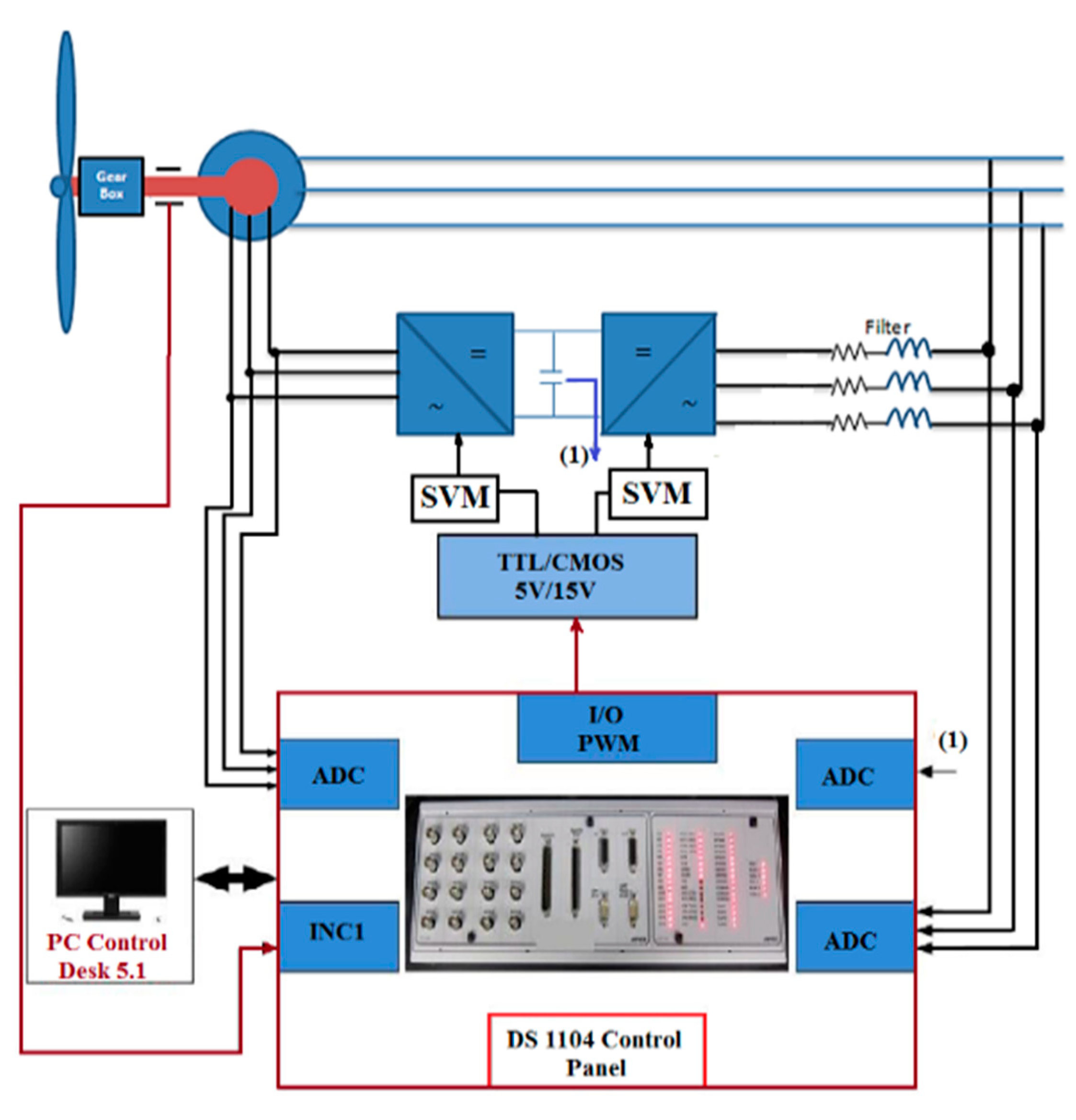
4. Experimental Setup

To validate the simulation results, a hardware laboratory experiment was performed using a DSpace 1104 board. A schematic of the laboratory setup is shown in Figure 20. The RSC and GSC gates switched from the DSpace 1104 output ports through the TTL/CMOS. The personal computer (PC) used a special chart to transfer data between hardware and software packages. The software packages were implemented through the modelling tool in Matlab/Simulink. The SO-AFLC was implemented using the fuzzy toolbox in Matlab, the real-time interface (RTI) in Simulink, and the Matlab/DSP library.

5. Experimental Results

The DS1104 control panel was used in the lab to implement the hardware test for the DFIG oscillating water column system, as depicted in Figure 21. The airflow speed was simulated using a DC motor directly coupled to the DFIG. The DC motor was controlled using a DC chopper circuit. A digital signal that reflected the rotor’s real speed was generated and supplied to the DS 1104 via an incremental encoder. Any measured data in the experiment were filtered before being supplied to the input ports of the DS1104 kit. So, noises were mitigated. The setup consisted of the following:

• A prime mover: 250 W, with servomotor, 180/220VDC, 3000 rpm.
• An incremental encoder: Speed: 1024 pulses, moment of inertia: 35 gcm², 6000 rpm.
• A DC chopper circuit: IR2110 IGBT 600V, 50A_sc, 1n5819 diode, 2060 MUR super rectifier.
• A DC motor: 180/220VDC, 3000 rpm.
• A voltage/current measurement device.
• The DFIG: 230/400 V, 270 W, 4 poles, 3.2/2 Amp, pf 1/0.75, 50 Hz.

Under random wave change, the DFIG oscillating water column power plant is investigated using SO-AFLC. The airflow speed was modelled using the DC motor and DC chopper circuit. The air flow speed inside the chamber is shown in Figure 22. The DFIG’s rotating speed is illustrated in Figure 23. Better speed tracking was achieved by both the AFLC and SO-AFLC compared to the PID, with a little improvement for the SO-AFLC (same as simulation results). Between t = 1.95 and t = 2.1 s, the SO-AFLC presented a faster dynamic response than the PID and AFLC. The SO-AFLC has a very low steady-state error in comparison to the AFLC and PID. In comparison to the PID and AFLC, the SO-AFLC enhanced the mechanical speed control by 21.12% and 15.35%, respectively. Figure 24 shows the mechanical power produced by the oscillating turbine. At the peak airflow speed, the SO-AFLC generates the highest power possible with the best power tracking. The power generated using the SO-AFLC (shown in Figure 24c) is higher than the power generated using the AFLC (Figure 24b) and PID (Figure 24a). The DC voltage between the RSC and GSC is shown in Figure 25. The SO-AFLC decreased the steady-state error in the DC link voltage by 2.13 volts in comparison to the AFLC and by 4.93 volts in comparison to the PID. When the chamber’s airflow speed reaches its maximum value (t = 2 s), the SO-AFLC regulates the DC voltage more effectively than the AFLC and PID.

The results obtained from the experiment are quite respectable when compared with the simulation results. The results reveal that the grid-tied OWCPP, based on DFIG performance, exhibits improved speed tracking, maximum power tracking, and extremely excellent DC voltage control when the SO-AFLC is employed as an alternative to a PID and AFLC.

6. Conclusions

This article proposes a SO-AFLC designed to enhance the performance of a grid-connected DFIG used in an oscillating water column power plant. The proposed SO-AFLC enhanced maximum power point tracking (MPPT), DC link voltage stability, and reactive power tracking for the DFIG system in the OWC power plant. Compared with the AFLC and PID, the SO-AFLC effectively prevents oscillations and overshooting. Experimental investigations were performed using a Dspace 1104 control board to validate the simulation results. The SO-AFLC demonstrates a faster response time, reduced undershooting, lower peak overshooting, and a very low steady-state error. Furthermore, the integral absolute error (IAE) index of the oscillating water column turbine was calculated to evaluate the feasibility of using the SO-AFLC, as opposed to the PID and/or AFLC, under identical conditions. The SO-AFLC shows superior performance in terms of speed tracking and power generation, with significant improvements in DC link voltage stability compared with both the AFLC and PID. The SO-AFLC has a mean square error that is reduced by 40.4% in comparison to the corresponding value derived from using the AFLC and by 84.9% in comparison to the corresponding value derived from using SGHS-PID. The efficiency of the grid-connected OWCPP was enhanced using the SO-AFLC compared to the PID and SO-AFLC. The average value of efficiency was improved to 93.5% using the SO-AFLC, compared to 91.1% for the AFLC and 83.21% for the PID. In conclusion, the SO-AFLC methodology has proved itself to be an effective control strategy for improving the performance of DFIG systems in OWC power plants, offering enhanced stability, efficiency, and power generation capabilities.

In future work, we plan to investigate the proposed SO-AFLC control model on a wind power plant in RAS GAREB, Gulf of Suez, Egypt. Similar to any other controller that uses integration, the SO-AFLC could encounter difficulties with wind-up in cases involving waves that have irregular amplitude profiles. Finally, the robustness of the proposed controller in terms of introducing noise into the airflow speed signal will be investigated in future work.

References

1. Mishra, S.K.; Purwar, S.; Kishor, N. Maximizing Output Power in Oscillating Water Column Wave Power Plants: An Optimization Based MPPT Algorithm. Technologies 2018, 6, 15. [Google Scholar] [CrossRef]
2. Drew, B.; Plummer, A.R.; Sahinkaya, M.N. A review of wave energy converter technology. Proc. Inst. Mech. E Part A J. Power Energy 2009, 223, 887–902. [Google Scholar] [CrossRef]
3. Napole, C.; Barambones, O.; Derbeli, M.; Cortajarena, J.A.; Calvo, I.; Alkorta, P.; Bustamante, P.F. Double Fed Induction Generator Control Design Based on a Fuzzy Logic Controller for an Oscillating Water Column System. Energies 2021, 14, 3499. [Google Scholar] [CrossRef]
4. Yang, L.; Xu, Z.; Ostergaard, J.; Dong, Z.Y.; Wong, K.P. Advanced control strategy of DFIG wind turbines for power system fault ride through. IEEE Trans. Power Syst. 2011, 27, 713–722. [Google Scholar] [CrossRef]
5. Yin, M.; Xu, Y.; Shen, C.; Liu, J.; Dong, Z.Y.; Zou, Y. Turbine stability-constrained available wind power of variable speed wind turbines for active power control. IEEE Trans. Power Syst. 2016, 32, 2487–2488. [Google Scholar] [CrossRef]
6. Abdellatif, W.S.; Hamada, A.; Abdelwahab, S.A.M. Wind speed estimation MPPT technique of DFIG-based wind turbines theoretical and experimental investigation. Electr. Eng. 2021, 103, 2769–2781. [Google Scholar] [CrossRef]
7. Lu, K.H.; Hong, C.M.; Han, Z.; Yu, L. New Intelligent Control Strategy Hybrid Grey–RCMAC Algorithm for Ocean Wave Power Generation Systems. Energies 2020, 13, 241. [Google Scholar] [CrossRef]
8. Pavel, C.C.; Lacal-Arántegui, R.; Marmier, A.; Schüler, D.; Tzimas, E.; Buchert, M.; Jenseit, W.; Blagoeva, D. Substitution strategies for reducing the use of rare earths in wind turbines. Resour. Policy 2017, 52, 349–357. [Google Scholar] [CrossRef]
9. Kumar, G.A.; Shivashankar. Optimal power point tracking of solar and wind energy in a hybrid wind solar energy system. Int. J. Energy Environ. Eng. 2022, 13, 77–103. [Google Scholar] [CrossRef]
10. Pang, B.; Dai, H.; Li, F.; Nian, H. Coordinated Control of RSC and GSC for DFIG System under Harmonically Distorted Grid Considering Inter-Harmonics. Energies 2020, 13, 28. [Google Scholar] [CrossRef]
11. Gogulamoodi, K.R.; Shaby, S.M.; Ramesh, P. Maximum power point tracking algorithm for grid-connected photo voltaic system. J. Phys. Conf. Ser. 2019, 1172, 012037. [Google Scholar] [CrossRef]
12. Bakhshi-Jafarabadi, R.; Sadeh, J.; Popov, M. Maximum power point tracking injection method for islanding detection of grid-connected photovoltaic systems in microgrid. IEEE Trans. Power Deliv. 2020, 36, 168–179. [Google Scholar] [CrossRef]
13. Medeiros, A.; Ramos, T.; de Oliveira, J.T.; Medeiros Júnior, M.F. Direct Voltage Control of a Doubly Fed Induction Generator by Means of Optimal Strategy. Energies 2020, 13, 770. [Google Scholar] [CrossRef]
14. Garrido, I.; Garrido, A.J.; Alberdi, M.; Amundarain, M.; Barambones, O. Performance of an ocean energy conversion system with DFIG sensorless control. Math. Probl. Eng. 2013, 2013, 260514. [Google Scholar] [CrossRef]
15. Alberdi, M.; Amundarain, M.; Garrido, A.; Garrido, I.; Casquero, O.; De la Sen, M. Complementary control of oscillating water column-based wave energy conversion plants to improve the instantaneous power output. IEEE Trans. Energy Convers. 2011, 26, 1021–1032. [Google Scholar] [CrossRef]
16. M’zoughi, F.; Garrido, I.; Garrido, A.J. Symmetry-breaking for airflow control optimization of an oscillating-water-column system. Symmetry 2020, 12, 895. [Google Scholar] [CrossRef]
17. M’zoughi, F.; Garrido, I.; Garrido, A.J.; De La Sen, M. Self-adaptive global-best harmony search algorithm-based airflow control of a wells-turbine-based oscillating-water column. Appl. Sci. 2020, 10, 4628. [Google Scholar] [CrossRef]
18. Salem, A.A.; Aldin, N.A.N.; Azmy, A.M.; Abdellatif, W.S. Implementation and validation of an adaptive fuzzy logic controller for MPPT of PMSG-based wind turbines. IEEE Access 2021, 9, 165690–165707. [Google Scholar] [CrossRef]
19. Gulzar, M.M.; Sibtain, D.; Murtaza, A.F.; Murawwat, S.; Saadi, M.; Jameel, A. Adaptive fuzzy based optimized proportional-integral controller to mitigate the frequency oscillation of multi-area photovoltaic thermal system. Int. Trans. Electr. Energy Syst. 2021, 31, e12643. [Google Scholar] [CrossRef]
20. Zeb, K.; Ali, Z.; Saleem, K.; Uddin, W.; Javed, M.; Christofides, N. Indirect field-oriented control of induction motor drive based on adaptive fuzzy logic controller. Electr. Eng. 2017, 99, 803–815. [Google Scholar] [CrossRef]
21. Zeb, K.; Islam, S.U.; Din, W.U.; Khan, I.; Ishfaq, M.; Busarello, T.D.C.; Ahmad, I.; Kim, H.J. Design of Fuzzy-PI and Fuzzy-Sliding Mode Controllers for Single-Phase Two-Stages Grid-Connected Transformerless Photovoltaic Inverter. Electronics 2019, 8, 520. [Google Scholar] [CrossRef]
22. Kochetkov, S.; Krasnova, S.A.; Utkin, V.A. The New Second-Order Sliding Mode Control Algorithm. Mathematics 2022, 10, 2214. [Google Scholar] [CrossRef]
23. Eker, I. Second-order sliding mode control with experimental application. ISA Trans. 2010, 49, 394–405. [Google Scholar] [CrossRef] [PubMed]
24. Alberdi, M.; Amundarain, M.; Maseda, F.; Barambones, O. Stalling behaviour improvement by appropriately choosing the rotor resistance value in Wave Power Generation Plants. In Proceedings of the 2009 International Conference on Clean Electrical Power, Capri, Italy, 9–11 June 2009; pp. 64–67. [Google Scholar]
25. Barambones, O.; Gonzalez de Durana, J.M.; Calvo, I. Adaptive Sliding Mode Control for a Double Fed Induction Generator Used in an Oscillating Water Column System. Energies 2018, 11, 2939. [Google Scholar] [CrossRef]
26. Jayashankar, V.; Udayakumar, K.; Karthikeyan, B.; Manivannan, K.; Venkatraman, N.; Rangaprasad, S. Maximizing power output from a wave energy plant. In Proceedings of the 2009 International Conference on Clean Electrical Power, Singapore, 23–27 January 2000; Volume 3, pp. 1796–1801. [Google Scholar]
27. Sarmento, A.; Gato, L.; Falcao, A.d.O. Turbine-controlled wave energy absorption by oscillating water column devices. Ocean Eng. 1990, 17, 481–497. [Google Scholar] [CrossRef]
28. Ghasemi, A.; Refan, M.H.; Amiri, P. Enhancing the performance of grid synchronization in DFIG-based wind turbine under unbalanced grid conditions. Electr. Eng. 2020, 102, 1175–1194. [Google Scholar] [CrossRef]
29. Döşoğlu, M.K. Nonlinear dynamic modeling for fault ride-through capability of DFIG-based wind farm. Nonlinear Dyn. 2017, 89, 2683–2694. [Google Scholar] [CrossRef]
30. Zamzoum, O.; Derouich, A.; Motahhir, S.; El Mourabit, Y.; El Ghzizal, A. Performance analysis of a robust adaptive fuzzy logic controller for wind turbine power limitation. J. Clean. Prod. 2020, 265, 121659. [Google Scholar] [CrossRef]
31. Talla, J.; Leu, V.Q.; Šmídl, V.; Peroutka, Z. Adaptive speed control of induction motor drive with inaccurate model. IEEE Trans. Ind. Electron. 2018, 65, 8532–8542. [Google Scholar] [CrossRef]
32. Benkahla, M.; Taleb, R.; Boudjema, Z. Comparative study of robust control strategies for a DFIG-based wind turbine. Int. J. Adv. Comput. Sci. Appl. 2016, 7, 2. [Google Scholar] [CrossRef]
33. Elnaghi, B.E.; Abelwhab, M.N.; Ismaiel, A.M.; Mohammed, R.H. Solar Hydrogen Variable Speed Control of Induction Motor Based on Chaotic Billiards Optimization Technique. Energies 2023, 16, 1110. [Google Scholar] [CrossRef]
34. Mohammed, R.H.; Ismaiel, A.M.; Elnaghi, B.E.; Dessouki, M.E. African vulture optimizer algorithm based vector control induction motor drive system. Int. J. Electr. Comput. Eng. 2023, 13, 2088–8708. [Google Scholar] [CrossRef]
35. Ratrey, R.; Dewangan, M.S.R. A Review on wind power generation using neural and fuzzy logic. Int. Res. J. Eng. Technol. 2021, 8, 0072–2395. [Google Scholar]
36. Sheng, W.; Li, H. A Method for Energy and Resource Assessment of Waves in Finite Water Depths. Energies 2017, 10, 460. [Google Scholar] [CrossRef]
Figure 1. Schematic diagram of the DFIG in OWCPP.
Electronics 13 00291 g001
Figure 2. OWC turbine characteristic curve.
Electronics 13 00291 g002
Figure 3. Synchronous q-d model of a DFIG.
Electronics 13 00291 g003
Figure 4. Block diagram of the AFLC.
Electronics 13 00291 g004
Figure 5. The membership functions for (a) inputs and (b) outputs.
Electronics 13 00291 g005
Figure 6. Block diagram of the SO-AFLC.
Electronics 13 00291 g006
Figure 7. Schematic diagram for the control model of the (a) RSC and (b) GSC.
Electronics 13 00291 g007
Figure 8. Air flow speed inside the chamber.
Electronics 13 00291 g008
Figure 9. Flow coefficient of the OWCPP.
Electronics 13 00291 g009
Figure 10. Rotor speed of the DFIG.
Electronics 13 00291 g010
Figure 11. Generated power.
Electronics 13 00291 g011
Figure 12. DC link voltage between the RSC and GSC.
Electronics 13 00291 g012
Figure 13. Grid reactive power.
Electronics 13 00291 g013
Figure 14. Air flow speed inside the chamber.
Electronics 13 00291 g014
Figure 15. Flow coefficient of the OWCPP.
Electronics 13 00291 g015
Figure 16. Mechanical rotor speed of the DFIG.
Electronics 13 00291 g016
Figure 17. Generated power.
Electronics 13 00291 g017
Figure 18. DC link voltage between the RSC and GSC.
Electronics 13 00291 g018
Figure 19. The efficiency of a grid-connected OWC turbine.
Electronics 13 00291 g019
Figure 20. Schematic detailing the hardware setup.
Electronics 13 00291 g020
Figure 21. Hardware experiment.
Electronics 13 00291 g021
Figure 22. Experimental air flow speed.
Electronics 13 00291 g022
Figure 23. Experimental mechanical rotor speed: (a) PID, (b) AFLC, and (c) SO-AFLC.
Electronics 13 00291 g023
Figure 24. Experimental power generated by the (a) PID, (b) AFLC, and (c) SO-AFLC.
Electronics 13 00291 g024
Figure 25. Experimental DC voltage between the GSC and RSC: (a) PID, (b) AFLC, and (c) SO-AFLC.
Electronics 13 00291 g025