Abstract
Accurate knowledge of oscillation parameters (i.e., frequency, amplitude, phase, and damping factor) is crucial for control strategies of power systems under power swing. This paper presents a method for the parameter estimation of power system oscillation signals under power swing based on Clarke–DFT. The proposed method provides accurate parameter estimation of damped sinusoidal signals for both balanced and unbalanced systems, which performs well even in the presence of harmonics. In the meantime, the negative frequency components in the spectra of the damped sinusoidal signals, which are caused by system imbalance, are calculated accurately using complex-valued interpolated DFT. To verify the performance of the proposed method, simulations are performed under balanced and unbalanced conditions. The results of the simulations confirm the effectiveness of the proposed method either in unbalanced or harmonic conditions.
1. Introduction
Power swing refers to a rapid and large-scale oscillation of power flow caused by power system disturbances such as faults, switching on/off large loads, generator disconnections, and line switching [1,2]. It can cause serious damage to the rotor shaft system of turbine generators or even threaten the safety and reliability of power grids [3,4]. Phasor measurement units (PMUs) are the cornerstone of intelligent sensing and monitoring of power systems [5]. They can be utilized for power quality classification [6,7], fault detection [8,9], and locating the fault location within the power system [10,11,12], which is crucial for the control strategy of power systems under power swing. However, the success of such applications lies in oscillation parameters (i.e., frequency, amplitude, phase, and damping factor) that can be accurately estimated [13,14,15,16].
Over the years, many techniques have been developed to estimate the parameters of power system signals more accurately, the majority of which are based on the Fourier algorithm. For example, one of the quickest estimators is the widely used one-cycle Fourier filter, which is also known as discrete Fourier transform (DFT), because it requires only one-cycle samples and is easy to implement. However, the one-cycle Fourier filter shows a deficiency when power systems are under power swing conditions [17,18]. Other well-known developed techniques for parameter estimation of power system signals include iterative DFT methods [19,20], the Kalman filter [21], the least-mean-square method [22], the improved Fourier algorithm [23,24], orthogonal filtering [25], the wavelet method [26], Taylor–Fourier transform (TFT) [27], and TFT-based enhanced versions [28,29,30,31,32].
Generally, the methods mentioned above can be used in three-phase systems by estimating the parameters of each phase independently, which means that they do not use the inherent relation between the three phases. In [33], the symmetrical properties of three-phase signals are utilized by space vector transformation (SVTFT). In [34], the three-phase fault during the power swing is detected by using zero-frequency filtering because the power swing is a balanced phenomenon. In [35], the symmetrical properties of power swing are considered for the identification of symmetrical faults. In [36], a new DFT-based algorithm is reported to estimate power system frequency under normal and fault conditions, which benefits from an optimization-based filter to eliminate harmonics. In [37,38,39], the Clarke transform is employed for the frequency estimation of three-phase power systems. It should be noted that a complex exponential signal will be obtained from three-phase oscillation signals under power swing by the Clarke transform.
Prony-based methods can be a choice for the parameter estimation of such a complex exponential signal [40]. However, Prony-based methods either require a prior order of the signal model or are sensitive to noise. Furthermore, the direct use of DFT for the estimation of such a complex exponential signal is not a good choice because the estimation error caused by spectral leakage and picket fence effects is large.
Windowed interpolation DFT (WIpDFT) [41,42] is an efficient tool for the accurate parameter estimation of sinusoid signals, which may use both the positive and negative frequency part of spectra. Although WIpDFT methods provide accurate estimation of amplitude, frequency, and phase, they are not applicable for the estimation of the damping factor, which is an important parameter of oscillation signals [43]. In [44], a damping IpDFT (DIDFT) algorithm is proposed, which can effectively estimate the parameters of damped signals and provide accurate results in single-tone signals. In [45], an IpDFT-based method, named Bertocco–Yoshida order 1 with leakage correction (BY1LC), is provided to estimate damped sinusoid signals with three spectral lines. Because of spectral leakage, these methods become rather impracticable if the signal consists of several frequency components. To overcome the negative influence of spectral leakage from harmonics, the Hanning window is adopted to improve the DIDFT method, which has been named the HDIDFT method [46].
In this paper, we propose a novel DFT-based method for estimating parameters of damped sinusoidal signals under both balanced and unbalanced conditions, which perform well even in the presence of harmonics. Compared with traditional DFT-based methods, the proposed method takes advantage of calculating complex-valued interpolated DFT bins. Therefore, the negative frequency components in the spectra of the damped sinusoidal signals are transformed into useful information to improve the accuracy of estimation, which are caused by the system’s imbalance and are ignored by traditional DFT-based methods. The accuracy of the proposed method is compared with the DIDFT, BY1LC, SVTFT, and HDIDFT. Related tests are designed according to the requirement of the IEC/IEEE 60255-118-1 standard [47]. The performance of the proposed method under either unbalanced or harmonic conditions is also compared with the HDIDFT and BY1LC methods. The simulation results show the superiority of the proposed method under either unbalanced or harmonic conditions.
The remainder of this paper is organized as follows: In Section 2, the signal model of the proposed method is introduced first. Then, parameter estimation under single-tone and multi-tone conditions is derived. In Section 3, simulations are performed under the instruction of the IEC/IEEE 60255-118-1 standard. Then, an IEEE 9-bus power system is simulated in PSCAD, and an asymmetrical fault is created to generate power swing under unbalanced conditions. The results show that the proposed method provides accurate estimations under power swing.
2. Parameter Estimation Based on Clarke–DFT
2.1. Signal Model
Power swings are defined as oscillations in active and reactive power flows on a transmission line caused by a large disturbance, such as power system faults, line switching, and generator disconnection. Generally, the system should be symmetric to maintain a stable state when a power swing or symmetrical fault occurs [35].
In [48,49,50], the damped sinusoid widely exists in power system transients (power swing and sub-synchronous oscillation), where the key of parameter estimation is damped signal analysis. To better characterize the dynamics of oscillating signals, we introduce the damping factor into a three-phase signal model.
Considering the symmetrical property of power swing, the oscillation signal is modeled as a set of symmetrical damped sinusoidal signals, which can be expressed as follows:
where A, τ, ϕ, and ω are amplitude, damping factor, phase, and normalized angular frequency, respectively. The subscripts represent each phase of the three-phase system. Assume that the signal y(n) is sampled at a sampling rate of fs = 1/Ts, where Ts represents the sampling interval.
The three-phase signal is routinely transformed by the orthogonal αβ0 transformation matrix (Clarke transform) into a zero-sequence y0 and the direct and quadrature-axis components, yα and yβ, as described in [51]:
It ensures that the amplitude of the system is invariant under this transformation. In practice, normally only the yα and yβ parts are used to form the complex signal ycomplex(n), given by [52]:
where A+ and A− are the amplitude of positive and negative sequences, respectively, and ϕ+ and ϕ− are the phases of positive and negative sequences, respectively.
Then, the original parameter estimation problem in a three-phase power system is converted into the parameter estimation problem of a set of complex exponentials.
2.2. Power System Oscillation Signal with Single Tone
In this subsection, a three-phase balanced condition is considered. Due to the properties of the Clarke transform, yα(n) and yβ(n) have an exactly 90-degree phase angle difference under balanced conditions. The amplitude of positive sequences, noted as A+ in (3), is equal to the three-phase system, while the amplitude of negative sequences, noted as A− in (3), is zero. Therefore, a complex signal can be obtained by combining yα(n) and yβ(n):
The novel estimation algorithm presented in this section aims to estimate A, τ, ϕ, and ω of the transformed exponential signal.
Weighting ycomplex(n) with a rectangular window of length N, we obtain an N-sample time sequence ycomplex(n) with n = 0, 1, 2, …, N − 1. The N-point DFT of ycomplex (n) can be expressed as follows:
where WN = e−j2π/N, k = 0, 1, …, N − 1. For the simplicity of expression, suppose λ = e(τTs+jω) and ρ = Aejϕ(1 − e(τTs+jω)N), so that (5) can be simplified as
Once λ and ρ are solved, the amplitude, damping factor, phase, and angular frequency can all be calculated. Multiplying both sides by the denominator on the right in (6) and rearranging the equation, we obtain the following:
The DFT bin Y(k) is given by a linear combination of the unknown parameters λ and ρ. There are two unknown parameters and N available equations for N > 2; by selecting two indexes with the largest and second-largest magnitudes, denoted as k1 and k2, it is possible to build a system of linear equations as follows:
where Y(k1) and Y(k2) represent DFT bins with the largest and second-largest magnitudes. λ and ρ can be obtained by solving the equation. The oscillation parameters can be calculated as shown below:
where imag(∙) denotes the imaginary part of its argument.
2.3. Power System Oscillation Signal with Multi Tones
Due to the integration of renewable energy, the electrical system is no longer strictly balanced and contaminated with harmonics. Therefore, the derivation in Section 2.2 is not applicable to unbalanced and harmonic situations if not adjusted. To extend the proposed method to unbalanced and harmonic conditions, an approach based on a multi-tone signal model is derived in this subsection. The unbalanced three-phase signal model with K harmonic components can be written as follows:
Such an unbalanced system problem causes Clarke’s transformed system signal to no longer represent a single complex exponential (positive sequence) that rotates anticlockwise at the fundamental system frequency in the complex plane, but an orthogonal sum of positive and negative sequences [53]. After applying the Clarke transform, the reconstructed complex signal can be written as follows:
where A+h and A−h are the amplitudes of the positive- and negative-sequence components of the hth-harmonic component, respectively. φ+h and φ−h are the phase angles of the positive- and negative-sequence components, respectively. By treating the negative frequency part as special harmonic components, the complex signal can be regarded as an H-tone complex exponential signal and (14) can be simplified as:
where H = 2K, an Ah, τh, ϕh, and ωh are the amplitude, damping factor, phase, and normalized angular frequency of the hth harmonic (including positive- and negative-sequence components), respectively. When h∈[1, K], each parameter corresponds to the positive sequence component. When h∈[K + 1, 2K], each parameter corresponds to the negative sequence component.
Weighting ycomplex(n) with a rectangular window of length N, we obtain an N-sample time sequence ycomplex(n) with n = 0, 1, 2…, N − 1. The DFT domain model of complex exponentials under harmonic conditions can be expressed as a linear superposition of different frequency components:
with and . Ah, τh, ϕh, and ωh are, respectively, the amplitude, damping factor, phase, and angular frequency of the hth harmonic. For h = 1, A1, τ1, ϕ1, and ω1 are the parameters of the fundamental component.
Merging the H rational functions in (16) into a single rational function, the denominator becomes the product of the H denominators . The numerator becomes an accumulation of merged denominator products without the hth contribution:
where the numerator and denominator can be expressed as:
From (18) and (19), it is clear that a0 = , b0 = 1 and that ah and bh are independent of k.
By multiplying both sides by the denominator, (17) can be rewritten as:
and by extracting the b0 = 1 from the accumulation, (20) can be written as:
and by rearranging (21),
Then, a linear equation is obtained as
where
According to the linear Equation (23), it is possible to build a 2H × 2H linear system with 2H unknowns. With N DFT samples and N > 2H, the unknown coefficients ah (h∈[0, H − 1]) and bh (h∈[1, H]) can be calculated by solving the linear equations:
From (19), it is obvious that a complex polynomial of degree H with bh can be formulated and it has a certain relation with λh. By multiplying both sides with and modifying the index expression of the left side, (19) can be reconstructed as follows:
By treating as unknown z, a polynomial can be formulated as
where the left-hand side is a polynomial of degree H and the right side indicates that this polynomial has H distinct roots λh. The parameters λh are the values of z satisfying the following:
Different from the relation between λh and bh, the parameters ρh are not easy to acquire from (18) directly. An alternate method based on (16) is more convenient for the solution of ρh. After the parameters λh are acquired, a linear system based on (16) is constructed as follows:
By utilizing H DFT samples, the parameters ρh can be acquired by solving the linear equations.
After the parameters λh and ρh are acquired, the damping coefficient, amplitude, phase, and angular frequency of the hth harmonic can be calculated by substituting λh and ρh into (9)–(12).
In the proposed method, the most important steps are solving the linear Equations (27) and (30). The selection of DFT samples is vital to the estimation results. Besides the peaks that represent harmonics, there are extra peaks caused by the noise under noisy conditions. If those extra peaks are not eliminated during the peak search procedure, it will increase unnecessary computational burden and introduce extra noise interference. According to the measurement requirements in the IEC/IEEE 60255-118-1 standard, harmonic components with amplitude greater than 1% of the fundamental are considered for harmonic interference. Therefore, spectral lines with amplitudes lower than 1% of the highest peak are ignored in the peak search procedure. To minimize the impact of noise, the optimum selection is made by several steps: The first step is identifying the peaks of spectral lines based on amplitude. Then, to filter out extra peaks, peaks with an amplitude lower than 1% of the highest peak are filtered out, which means that if the amplitudes of the peaks are less than 1% of the fundamental amplitude, they will be treated as noise and ignored. Finally, find two spectral lines with a local maximum amplitude around each remaining peak. The flow chart of the proposed method is shown in Figure 1.
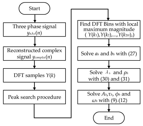
Figure 1.
Flow chart of the proposed method.
2.4. Computational Complexity Analysis
The computational complexity of the proposed method mainly consists of three parts. The first part is calculating the DFT bins of a reformed complex signal ycomplex(n) of which the length is N. So, the time complexity of DFT is O(Nlog2N). The second part is the solution of linear Equations (27) and (31). (27) is a 2H × 2H linear system while (31) is an H × H linear system. So the time complexity of solving (27) and (31) is O((2H)3) and O(H3), respectively. The last part is to solve the roots of the H-order polynomial (29) and the time complexity is O(Hlog2H). Therefore, the time complexity of the proposed method can be expressed as O(Nlog2N) + O((2H)3) + O(H3) + O(Hlog2H). The average running time of this method in Matlab is less than 0.005 s, and the laptop configuration is (CPU: core i7, memory: 8 GB).
3. Simulation Results
Several simulations are provided in this section. The first part is the assessment of the proposed method’s performance under a steady state. Both balanced and unbalanced conditions are considered. The accuracy of the proposed method is compared with the DIDFT method, the HDIDFT method, the BY1LC method, and the Cramer–Rao lower bounds (CRLB). The second part reports test results under the instruction of the latest standard IEC/IEEE 60255-118-1. Both the steady-state compliance test and dynamic test are performed, and the proposed method is also compared with the SVTFT method [33], which is a state-of-the-art method of dynamic phasor estimation. The third part is the validation of the proposed method under complex harmonic conditions. The last part is the validation of the proposed method in an IEEE 9-bus power system under power swing conditions, simulated in PSCAD [54].
3.1. Steady-State Tests under Balanced and Unbalanced Conditions
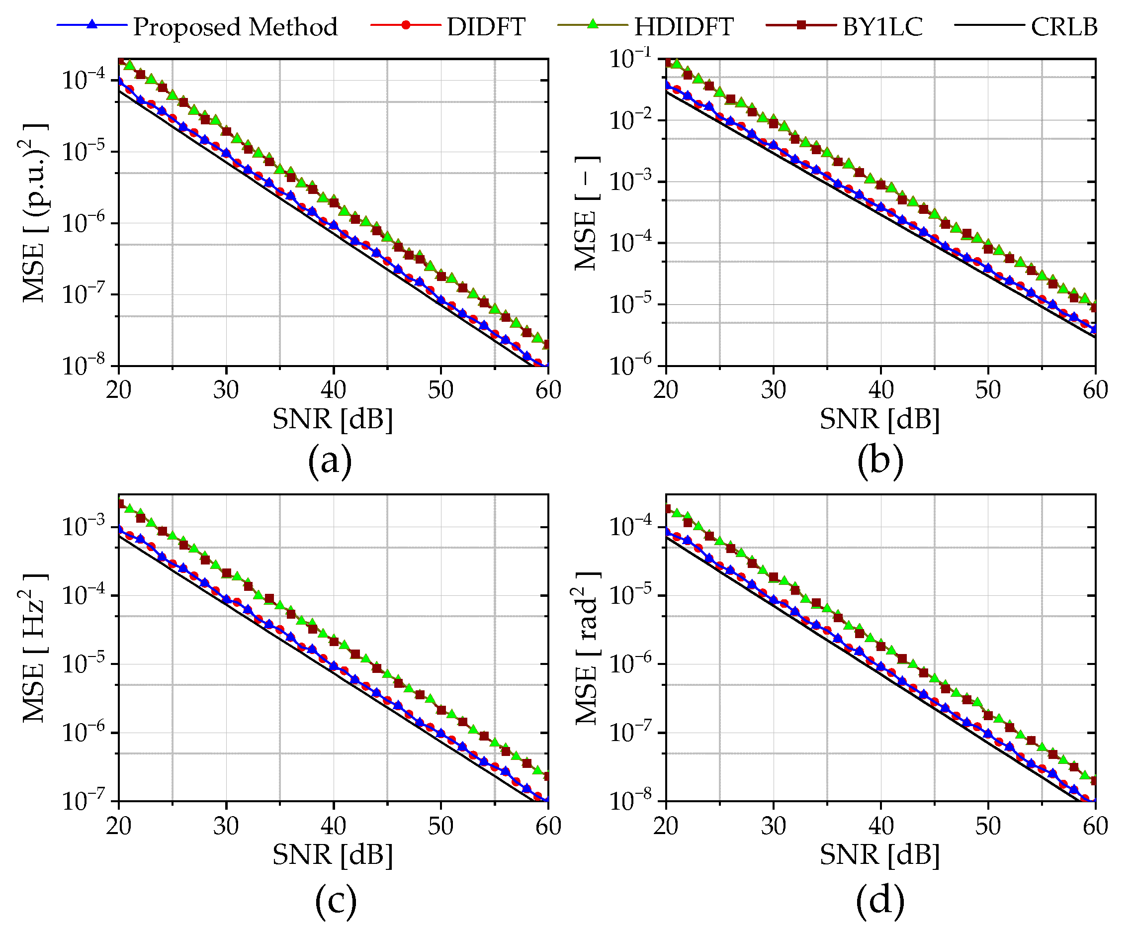
In this subsection, the performance of the proposed method is evaluated by simulations with different Signal–Noise Ratios (SNRs) and values of the cycle in the range (CiR), where CiR = Nf/fs. The mean squared error (MSE) is used to evaluate the performance of the methods. The number of independent trials is set as 3000 and averaged to obtain the results.
First, a balanced three-phase signal is generated, the frequency is set as f = 51 Hz, the amplitude of the test signal is set as A = 1, the damping factor is set as τ = −0.1, the initial phase is set as ϕ = 0.1, and the sampling frequency fs is set as 3 kHz. The window length is set as N = 256 and the SNR varies from 20 dB to 60 dB. The MSEs of estimations are reported in Figure 2.
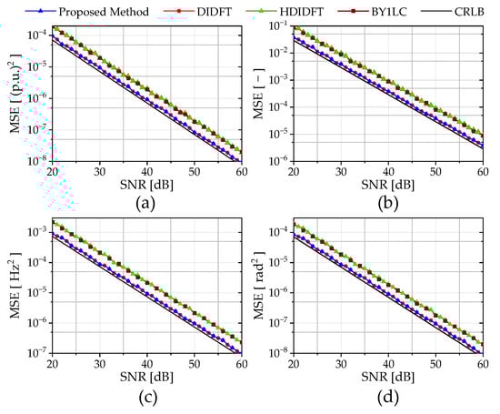
Figure 2.
Performance of estimation under balanced conditions. (a) Amplitude. (b) Damping factor. (c) Frequency. (d) Phase.
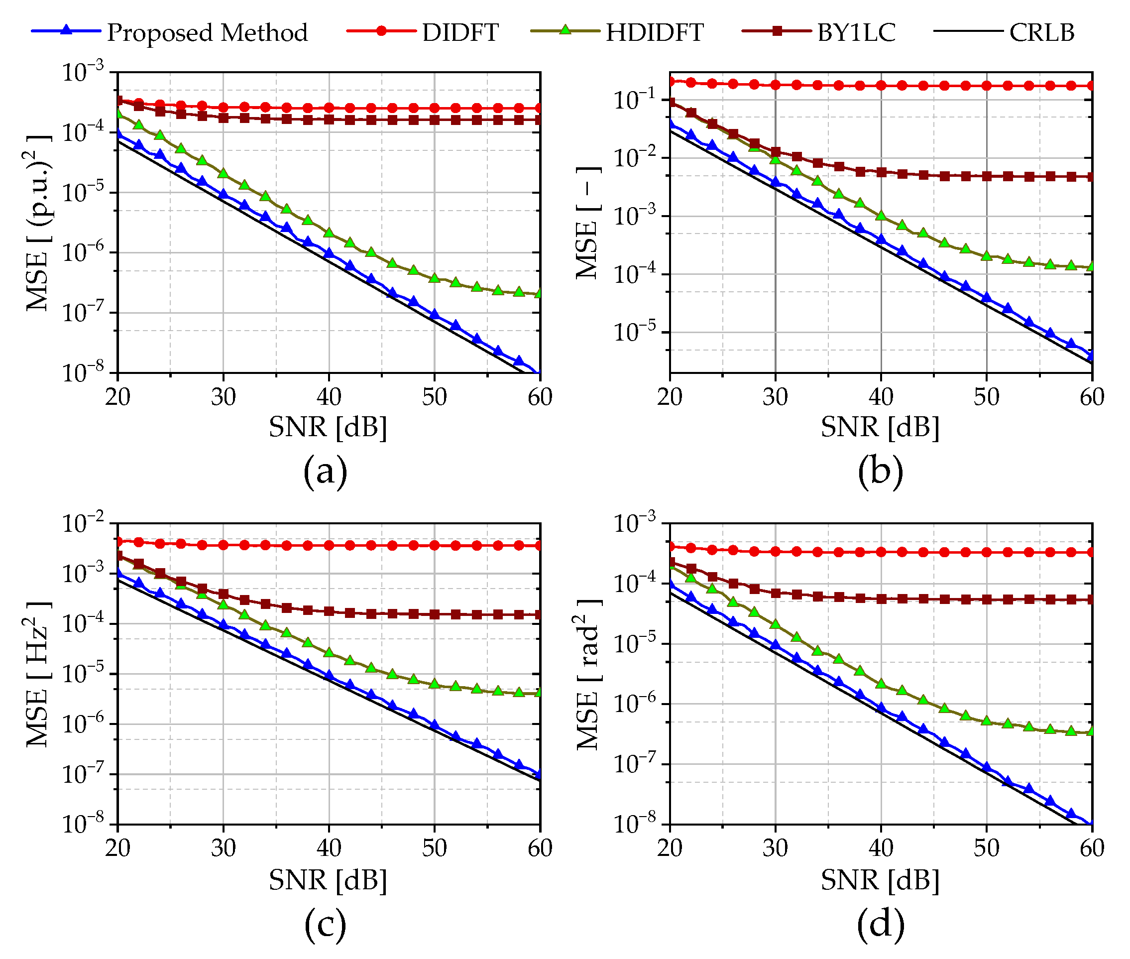
Then, an unbalanced three-phase signal is generated. The effect of unbalance is reflected by setting A+ = 1, A− = 0.3 and other parameters are the same as the balanced condition. The MSE of estimation is reported in Figure 3.

Figure 3.
Performance of estimation under unbalanced conditions. (a) Amplitude. (b) Damping factor. (c) Frequency. (d) Phase.
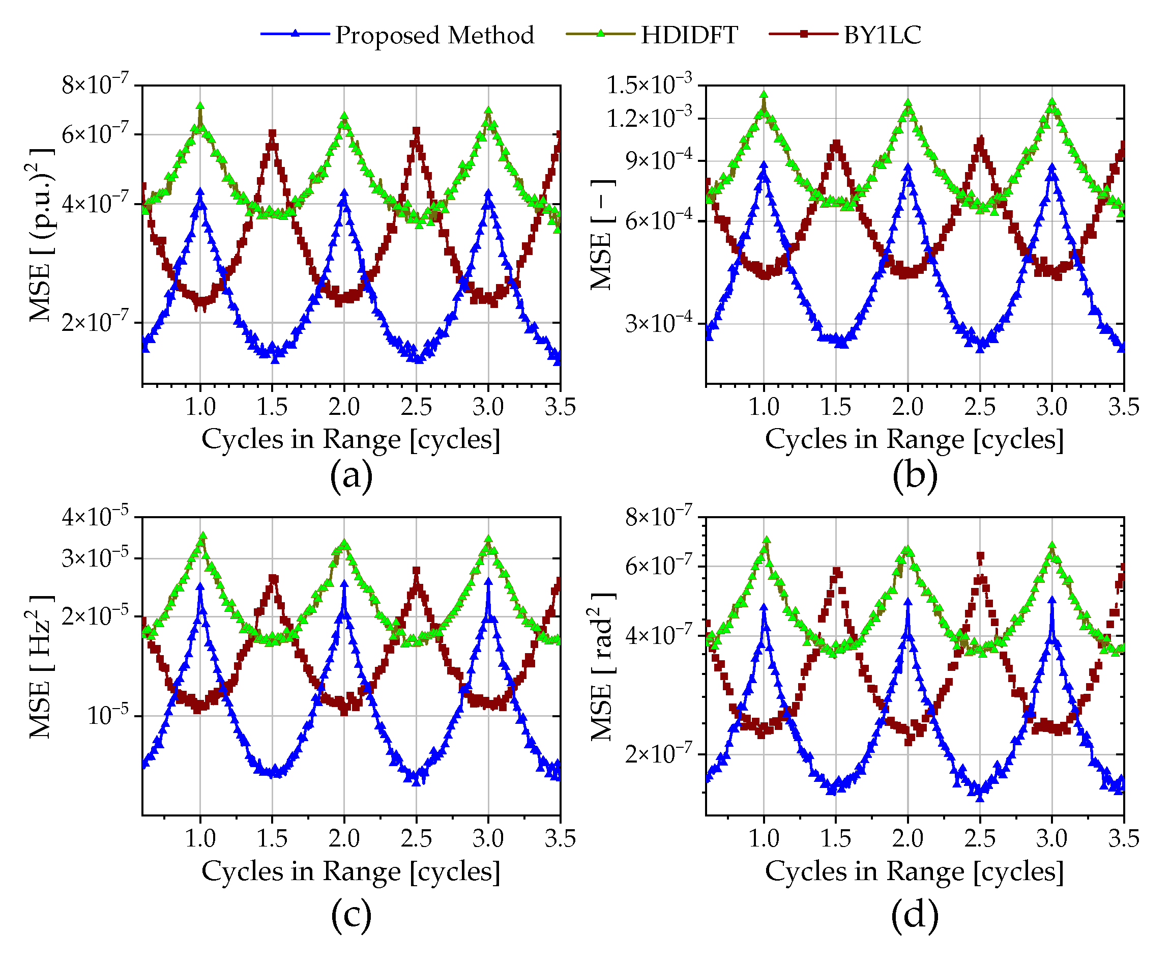
Finally, the CiR test is performed. A balanced three-phase signal is generated. The amplitude of the test signal is A = 1, the damping factor is τ = −0.1, the initial phase is ϕ = 0.1, and the sampling frequency fs is set as 3 kHz. The observation window length is set as N = 128. The CiR ranges from 0.5 to 3.5 nominal cycles and the SNR is set to 50 dB. The MSE of estimates is reported in Figure 4.
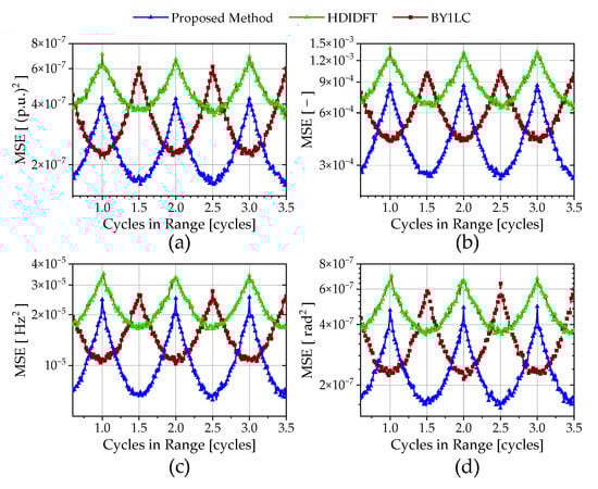
Figure 4.
Performance of estimation with different CiRs. (a) Amplitude. (b) Damping factor. (c) Frequency. (d) Phase.
Under balanced conditions, there is no negative frequency component in the reconstructed complex signal, which means that noise is the major factor affecting the accuracy of the results. Because both the DIDFT and the proposed method use a rectangular window, the results of the proposed method and the DIDFT method are approximately the same and close to the CRLB. As known, the rectangular window has the smallest equivalent noise bandwidth, so the proposed method and the DIDFT method outperform the HDIDFT and BY1LC methods.
Under unbalanced conditions, due to the spectral leakage from the negative frequency component, the accuracy of the DIDFT and the BY1LC are hardly improved with an increase in the SNR. The HDIDFT method restrains the spectral leakage by applying the Hann window, so its performance is much better than the DIDFT method. However, the accuracy shows little improvement when the SNR is higher than 50 dB. The proposed method outperforms competitors and its accuracy continues to improve with an increase in the SNR.
The result in Figure 4 demonstrates that the proposed method offers an accurate estimate when the observation window length is less than one nominal cycle under noisy situations. This indicates that the proposed method can achieve a good time resolution. In the case of synchronous full-cycle sampling, there is only one DFT bin available for the single-tone signal while HDIDFT and the proposed method require two DFT bins. So, in the noisy condition, those two methods are more sensitive to noise when the CiR is an integer.
3.2. Test under IEC/IEEE 60255-118-1 Standard
3.2.1. Steady-State Compliance Tests
In this part, steady-state compliance tests are designed according to the instructions of the IEC/IEEE 60255-118-1 standard. These tests under steady-state conditions include three items: (1) off-nominal frequency (f ranges from 45 Hz to 55 Hz), (2) single harmonic distortion (10% of each harmonic up to 50th), (3) interharmonic interference (10% of input signal magnitude; frequency of interharmonic is set as 25 Hz and 75 Hz).
The sampling frequency is set as 5 kHz and the SNR is set to 50 dB. The SVTFT requires a window length with an odd number, so the window length of SVTFT is set to 257 while the other three methods are set to 256. The results of Frequency Error (FE), Rate of Change of Frequency Error (RFE), and Total Vector Error (TVE) are listed in Table 1, Table 2 and Table 3. The test results show that the proposed method is more accurate than the other methods under off-nominal frequency conditions. Under single harmonic distortion, the HDIDFT method provides the best results. Under interharmonic conditions, the BY1LC method provides good FE results, but the TVE is not satisfactory. The performance of the proposed method and the SVTFT method are at the same level under interharmonic conditions.

Table 1.
Results under off-nominal frequency conditions.
Table 2.
Results under harmonic distortions.
Table 3.
Results under interharmonic conditions.
To be mentioned, the proposed method, BY1LC, and HDIDFT are not specifically designed for dynamic phasor measurement, and the direct estimation of ROCOF (Rate of Change of Frequency) is not given. So, the RFEs of these three methods are not listed in the Tables of results.
3.2.2. Amplitude and Phase Modulation Tests
Three-phase voltage signals are modeled by modulating their amplitudes with ±0.1 per unit sinusoidal variation of f1 = 2.0 Hz. The Clarke-transformed three-phase signal is expressed as (32). The amplitude parameters are set as A+ = 1, A− = 0.3 to reflect the unbalance effect. The simulation is performed at the nominal frequency f = 50 Hz.
where
The sampling frequency is set as 6 kHz and the observation window length is set to 256 samples (N = 256), and 255-sample overlap is considered between adjacent observation windows. The test signals are added with white Gaussian noise and SNR = 50 dB.
The TVE, which represents phasor estimation error, is indicated in the IEEE Standard as
where Xr and Xe are the true and estimated values of the phasor, respectively.
Table 4 reports the FE, RFE, and TVE results. Figure 5 reports the maximum TVE of each fundamental cycle. From Figure 5, it is obvious that the SVTFT provides the best results for the amplitude and phase-modulated signal due to its excellent dynamic performance. Although the proposed method is not as good as the SVTFT method, it outperforms the other two methods. The maximum TVE returned by the proposed method is lower than 0.6%. In the meantime, the maximum TVE offered by HDIDFT is about 0.9%. For the overall behavior as reported in Figure 5, the proposed method can reduce the TVE by 30% compared with HDIDFT.
Table 4.
Results under amplitude and phase-modulation conditions.
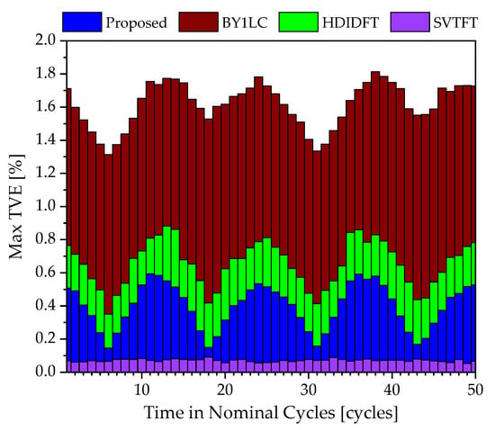
Figure 5.
Max TVE values of methods under amplitude and phase modulation.
3.2.3. Amplitude and Phase Step Tests
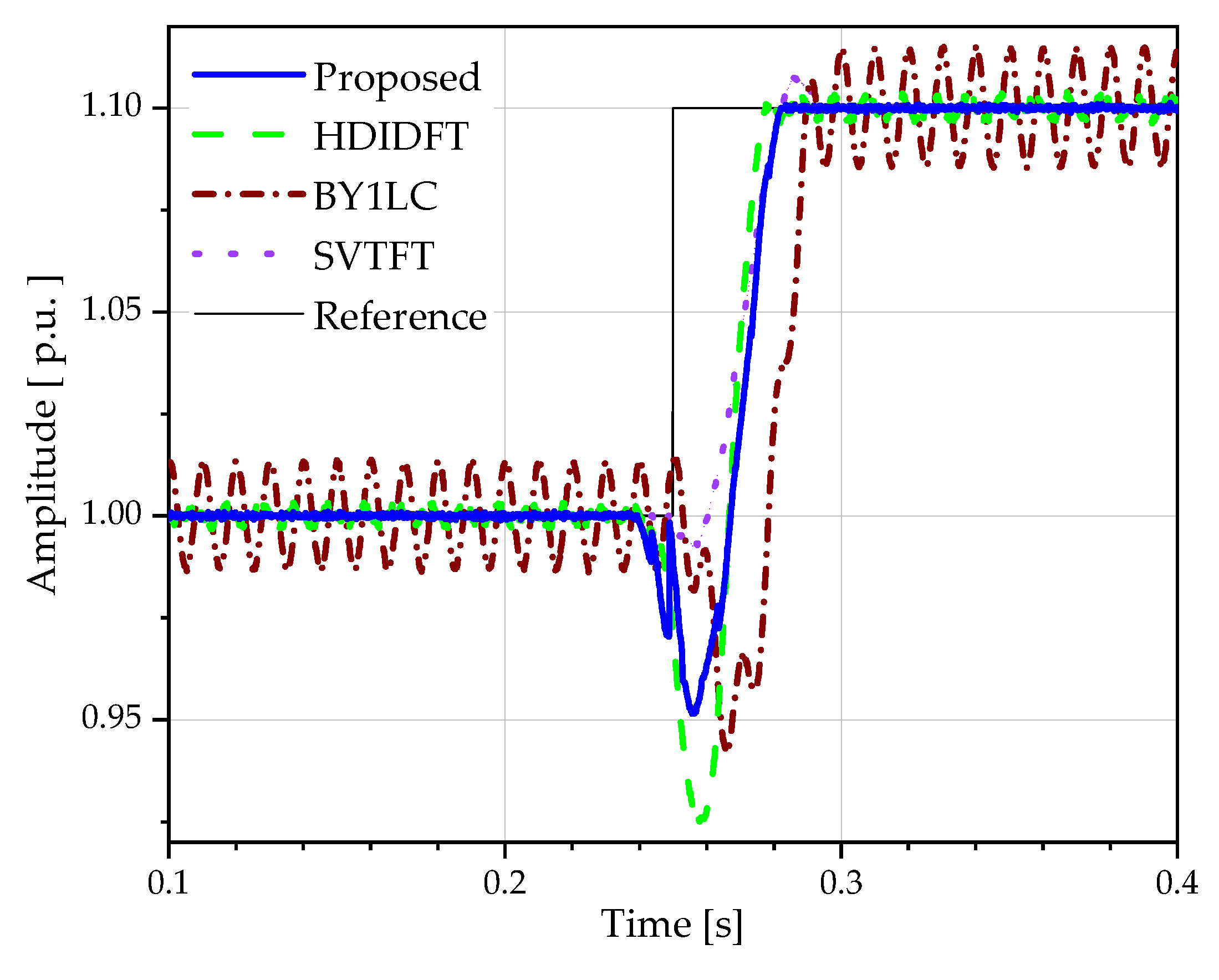
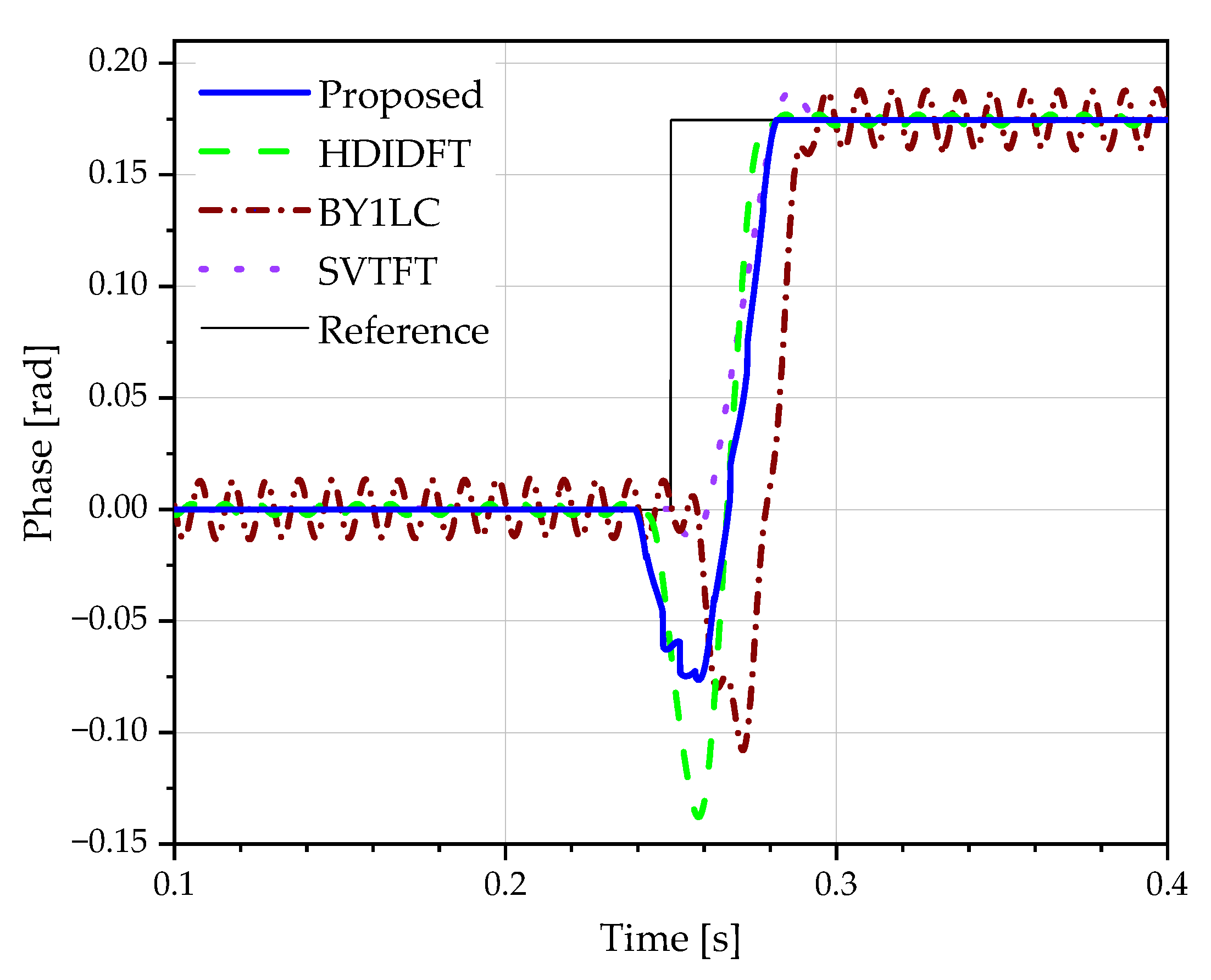
To assess the dynamic behavior of the proposed method, one of the dynamic benchmarks based on amplitude and phase step change is adopted in this part. Unbalance among three-phase signals is reflected by setting A+ = 1, A− = 0.3. An amplitude step-change signal with a step size of 10% of the amplitude and a phase step-change signal with a step size of π/18 are used for simulations.
The sampling frequency is set as 6 kHz and the window length is set to 256 samples (N = 256) and 255-point overlap is used between adjacent windows. The signal is corrupted with a Gaussian noise of 60 dB SNR. The simulation results of this test case are shown in Figure 6 and Figure 7. According to Figure 6 and Figure 7, the SVTFT method provides the best results due to its excellent dynamic performance. The results of the other three competitors show a deviation at the instant of the step occurring. The proposed method shows less overshoot and better stability than the HDIDFT and BY1LC methods.
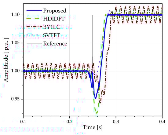
Figure 6.
Amplitude-tracking behavior under step conditions.

Figure 7.
Phase-tracking behavior under step change conditions.
3.2.4. Frequency Ramp Tests
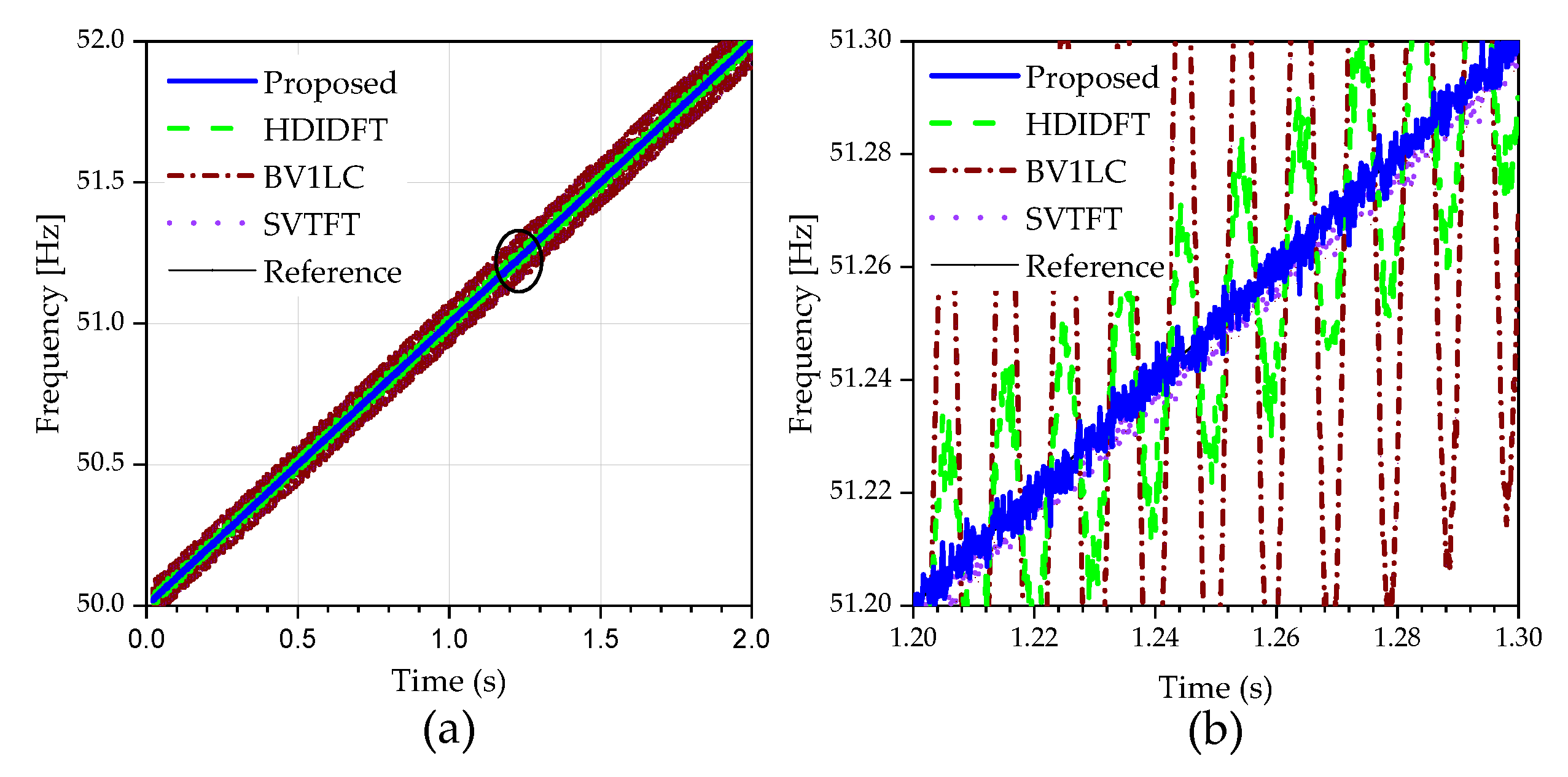
To evaluate the dynamic behavior of the proposed method, one of the dynamic benchmarks based on frequency ramp is adopted. The rate of frequency ramp is set to 1.0 Hz/s and the fundamental frequency varies from 50 to 52 Hz as specified in the IEEE C37.118.1-2011 standard. Unbalance among three-phase signals is reflected by setting A+ = 1, A− = 0.3. The sampling frequency is set to 6 kHz. The observation window length is set to 256 samples (N = 256) and 255-point overlap is used between adjacent windows. The SNR is set as 50 dB. The test results are reported in Table 5 and Figure 8; it is obvious that the proposed method provides more accurate results during the ramp compared with other methods.
Table 5.
Results under frequency ramp tests.
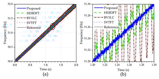
Figure 8.
(a) Frequency estimation during ramp. (b) Zoomed view of the circled area in (a).
3.3. Parameter Estimation with Harmonics
To validate the effectiveness of the proposed method under unbalanced harmonic conditions, a simulation is performed in MATLAB [55]. In this simulation, a set of unbalanced three-phase signals containing several harmonic components is generated and the parameters of the harmonics are listed in Table 6.
Table 6.
Component parameters of the simulated harmonic signal.
The fundamental frequency f1 is 53 Hz, the sampling frequency fs is 6 kHz, the window length N is 512, and the SNR is set to 50 dB. The performance of the proposed method under harmonic conditions is compared with HDIDFT and BY1LC. The MSEs of the amplitude, frequency phase, and damping factor of the harmonics are listed in Table 7. By comparing the MSEs of estimated results, it is obvious that the overall performance of the proposed method is better than the other two methods under unbalanced harmonic conditions.
Table 7.
Harmonic estimation results of different methods.
Both the proposed method and the HDIDFT method are based on the characteristics of spectral lines in the frequency domain. The HDIDFT method focuses on suppressing spectral leakage and harmonic interference by applying the Hanning window, but for the multi-tone signals of a power system, the spectral leakage and harmonic interference may not be effectively suppressed, and weak harmonic components can easily be obscured by nearby strong harmonics due to the spectral leakage. It can be seen from the results that the estimates of second-harmonic parameters provided by HDIDFT and BY1LC are very unsatisfactory, especially the damping factor, which has an unacceptable error. The proposed method takes every frequency component into consideration, which improves the accuracy of parameter estimation in the presence of harmonics. Therefore, the proposed method outperforms HDIDFT and BY1LC, especially in the results of the second harmonic.
3.4. Parameter Estimation of Oscillation Signal with Power Swing
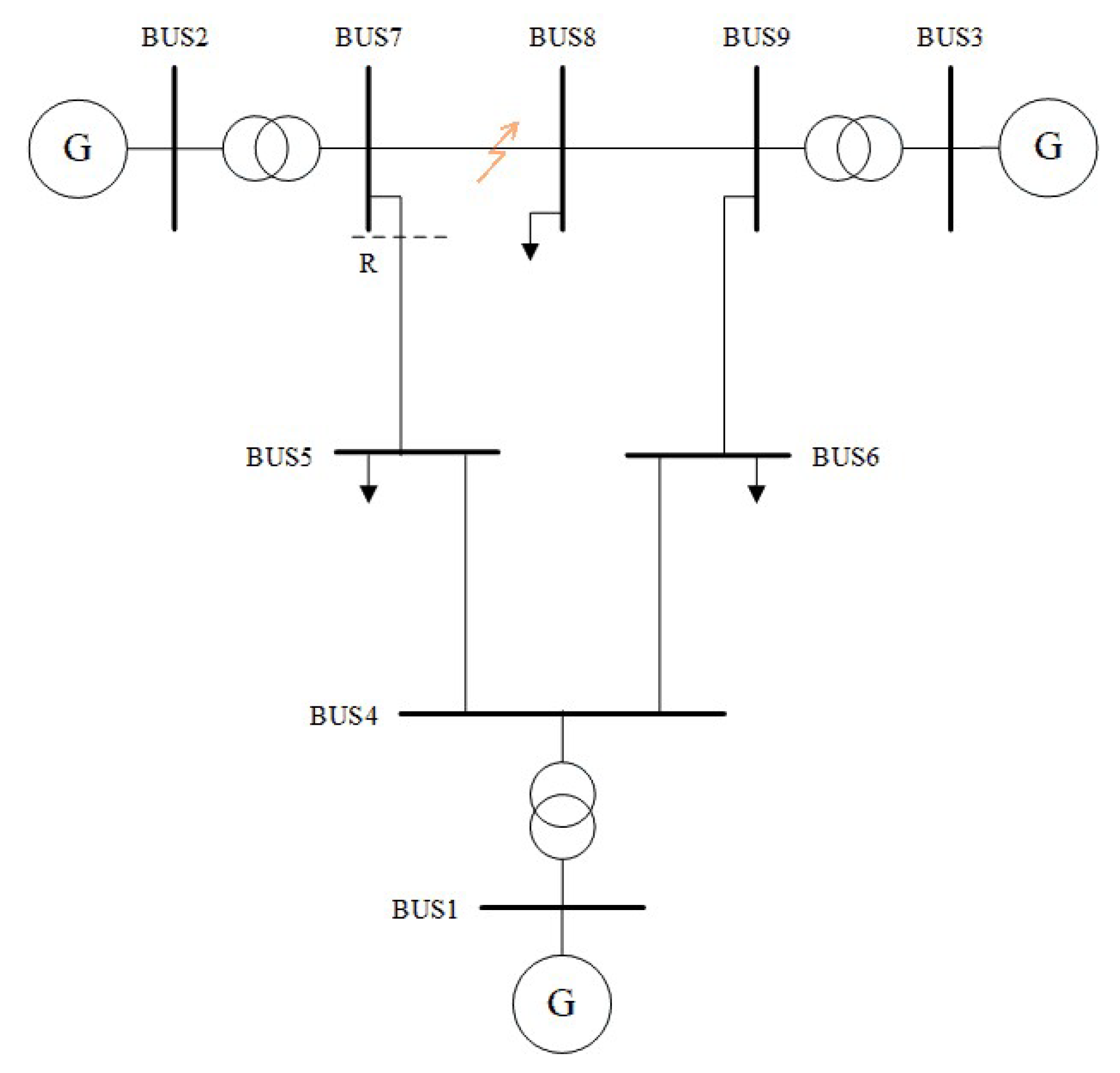
To exhibit the effectiveness of the proposed method when a power swing happens, the classical IEEE 9-bus power system model is selected as shown in Figure 9. The system is simulated in PSCAD software 4.6.0 [54]; detailed information about the system can be found in [56,57]. In this simulation, a distance relay is installed between bus-7 and bus-5. To create an unbalanced power swing, a phase-AB-to-ground fault is created in the line between bus-7 and bus-8. The fault is initiated at t = 1 s and cleared after 0.2 s by opening circuit breakers located at the ends of this line. The oscillation signal is observed using the distance relay R.
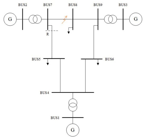
Figure 9.
Diagram of the adopted IEEE 9-bus power system.
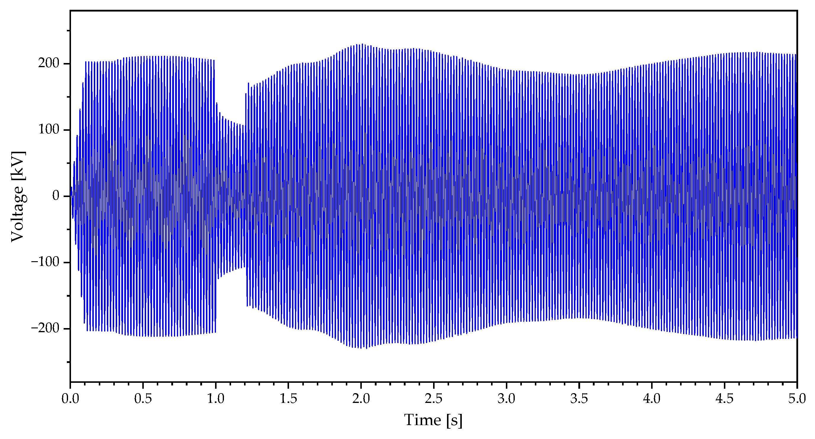
The sampling rate of the distance relay is set to 5 kHz and the waveform is processed in MATLAB. The voltage waveform of phase A is depicted in Figure 10. In addition, the length of the observation window is 1.28 nominal cycles, so there are 128 samples (N = 128) in each observation window. The three-phase voltage signal recorded by the relay R is used to evaluate the proposed method and competitors.
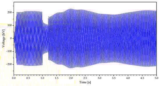
Figure 10.
Voltage waveform of phase A in the IEEE 9-bus system under power swing.
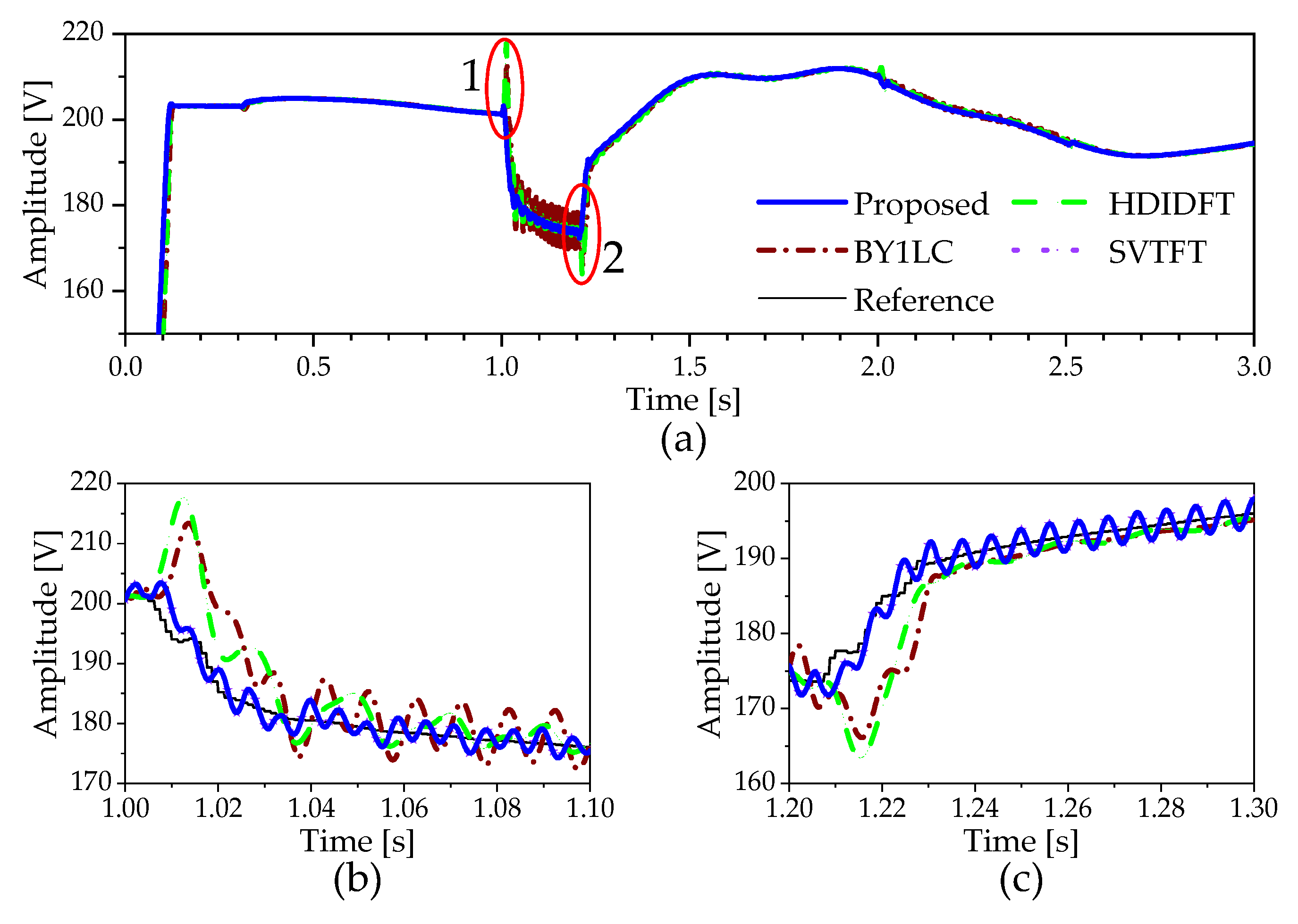
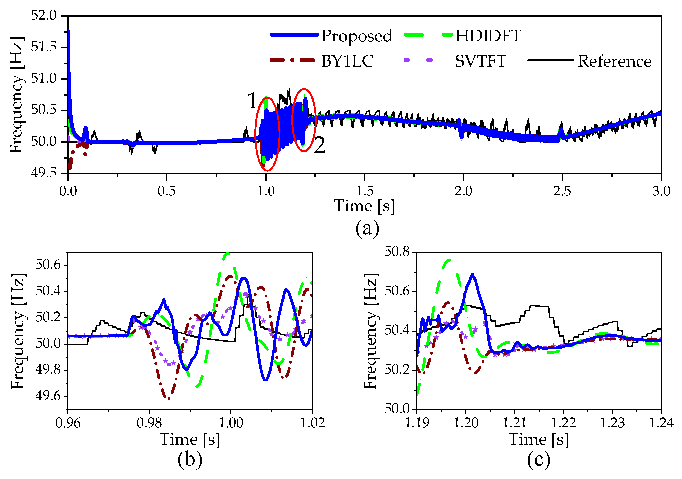
The proposed method has been compared with the other three competitors. The amplitude and frequency estimation results are reported in Figure 11 and Figure 12. The proposed method can track the amplitude variation during the dynamic process. During the fault, the test results of all methods show a fluctuation around the reference value. When the fault occurs or is removed, the proposed method can track the true value appropriately after a nominal period and the overshoot of the proposed method is lower than HDIDFT and BY1LC.4.
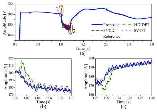
Figure 11.
Comparison of amplitude measurement results offered by methods. (a) Overall view of the estimated amplitude; (b) Zoomed view of the fault occurrence corresponding to red circle 1 in (a); (c) Zoomed view of the fault removal corresponding to red circle 2 in (a).
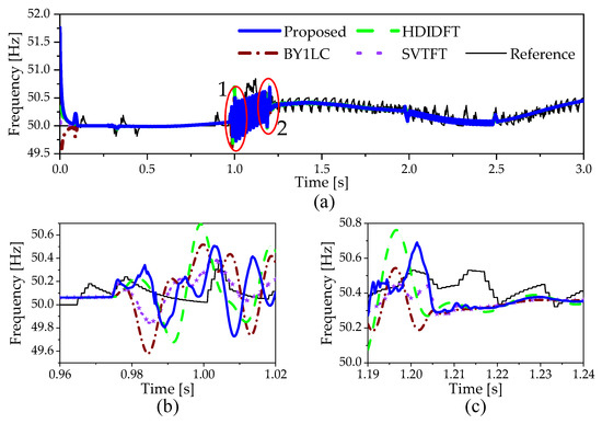
Figure 12.
Comparison of frequency measurement results offered by methods. (a) Overall view of the estimated frequency; (b) Zoomed view of the fault occurrence corresponding to red circle 1 in (a); (c) Zoomed view of the fault removal corresponding to red circle 2 in (a).
4. Conclusions
A Clarke transform-based complex-valued DFT method has been proposed in this article. The proposed method achieves accurate measurement of oscillation signal parameters. By applying the Clarke transform, the original oscillation parameter estimation problem in a three-phase power system is transformed into the parameter estimation problem of a set of complex exponentials. Then, with a complex-valued interpolated DFT-based algorithm, the proposed method is applied to either unbalanced or harmonic conditions. By comparing with other methods, it shows that the proposed solution can offer accurate estimates under noisy conditions. The performance of the proposed method under either unbalanced or harmonic conditions has been also evaluated, and the results show that the parameters of damped sinusoidal signals can be estimated accurately by using the proposed method. Further work will focus on two aspects: (1) improving the dynamic behavior of the proposed method and deriving a single-phase solution of the proposed method based on phase shifting; (2) incorporating a window (e.g., Hanning) to weighted the input samples and derive new parameter estimation formulas, which aim to reduce the mutual interference between the multi tones of unbalanced signals.
Author Contributions
Conceptualization, J.S. and X.S.; Methodology, J.S., X.S., J.Z. and H.W.; Writing—original draft, J.S. and X.S.; Writing—review and editing, J.Z. and H.W.; Supervision, J.Z. and H.W.; Funding acquisition, J.Z. All authors have read and agreed to the published version of the manuscript.
Funding
This work was supported in part by the Hunan Provincial Natural Science Foundation of China under Grant No. 2023JJ30197 and the Changsha Natural Science Foundation under Grant No. kq2208057.
Data Availability Statement
The data that support the findings of this study are available from the corresponding author upon reasonable request.
Conflicts of Interest
The authors declare no conflicts of interest.
References
- Wandhare, R.G.; Agarwal, V. Novel Stability Enhancing Control Strategy for Centralized PV-Grid Systems for Smart Grid Applications. IEEE Trans. Smart Grid 2014, 5, 1389–1396. [Google Scholar] [CrossRef]
- Hashemi, S.M.; Sanaye-Pasand, M.; Shahidehpour, M. Fault Detection During Power Swings Using the Properties of Fundamental Frequency Phasors. IEEE Trans. Smart Grid 2019, 10, 1385–1394. [Google Scholar] [CrossRef]
- Liu, H.; Xie, X.; Li, Y.; Liu, H.; Hu, Y. Mitigation of SSR by embedding subsynchronous notch filters into DFIG converter controllers. IET Gener. Transm. Distrib. 2017, 11, 2888–2896. [Google Scholar] [CrossRef]
- Xie, X.; Zhan, Y.; Liu, H.; Li, W.; Wu, C. Wide-area monitoring and early-warning of subsynchronous oscillation in power systems with high-penetration of renewables. Int. J. Electr. Power Energy Syst. 2019, 108, 31–39. [Google Scholar] [CrossRef]
- Song, J.; Zhang, J.; Kuang, H.; Wen, H. Dynamic Synchrophasor Estimation Based on Weighted Real-Valued Sinc Interpolation Method. IEEE Sens. J. 2023, 23, 588–598. [Google Scholar] [CrossRef]
- Zhu, K.; Teng, Z.; Qiu, W.; Tang, Q.; Yao, W. Complex Disturbances Identification: A Novel PQDs Decomposition and Modeling Method. IEEE Trans. Ind. Electron. 2023, 70, 6356–6365. [Google Scholar] [CrossRef]
- Ma, J.; Liu, J.; Qiu, W.; Tang, Q.; Wang, Q.; Li, C.; Peretto, L.; Teng, Z. An Intelligent Classification Framework for Complex PQDs Using Optimized KS-Transform and Multiple Fusion CNN. IEEE Trans. Ind. Inform. 2023, 1–10. [Google Scholar] [CrossRef]
- Mirshekali, H.; Dashti, R.; Keshavarz, A.; Shaker, H.R. Machine Learning-Based Fault Location for Smart Distribution Networks Equipped with Micro-PMU. Sensors 2022, 22, 945. [Google Scholar] [CrossRef]
- Theodorakatos, N.P.; Lytras, M.D.; Kantoutsis, K.T.; Moschoudis, A.P.; Theodoridis, C.A. Optimization-based optimal PMU placement for power state estimation and fault observability. In Proceedings of the 11th International Conference on Mathematical Modeling in Physical Sciences, Belgrade, Serbia, 5–8 September 2022. [Google Scholar]
- Alexopoulos, T.A.; Manousakis, N.M.; Korres, G.N. Fault Location Observability using Phasor Measurements Units via Semidefinite Programming. IEEE Access 2016, 4, 5187–5195. [Google Scholar] [CrossRef]
- Kezunovic, M. Smart Fault Location for Smart Grids. IEEE Trans. Smart Grid 2011, 2, 11–22. [Google Scholar] [CrossRef]
- Theodorakatos, N.P. Fault Location Observability Using Phasor Measurement Units in a Power Network Through Deterministic and Stochastic Algorithms. Electr. Power Components Syst. 2019, 47, 212–229. [Google Scholar] [CrossRef]
- Ashrafian, A.; Mirsalim, M.; Masoum, M.A.S. An Adaptive Recursive Wavelet Based Algorithm for Real-Time Measurement of Power System Variables During Off-Nominal Frequency Conditions. IEEE Trans. Ind. Inform. 2018, 14, 818–828. [Google Scholar] [CrossRef]
- Rao, J.G.; Pradhan, A.K. Accurate Phasor Estimation During Power Swing. IEEE Trans. Power Deliv. 2016, 31, 130–137. [Google Scholar] [CrossRef]
- Jafarpisheh, B.; Madani, S.M.; Parvaresh, F. Phasor Estimation Algorithm Based on Complex Frequency Filters for Digital Relaying. IEEE Trans. Instrum. Meas. 2018, 67, 582–592. [Google Scholar] [CrossRef]
- Zhao, D.; Li, S.; Wang, F.; Zhao, W.; Huang, S. Estimation of Wideband Multi-Component Phasors Considering Signal Damping. Sensors 2023, 23, 7071. [Google Scholar] [CrossRef] [PubMed]
- Barchi, G.; Macii, D.; Petri, D. Accuracy of one-cycle DFT-based synchrophasor estimators in steady-state and dynamic conditions. In Proceedings of the 2012 IEEE International Instrumentation and Measurement Technology Conference Proceedings, Graz, Austria, 13–16 May 201; pp. 1529–1534.
- Shan, X.; Macii, D.; Petri, D.; Wen, H. Enhanced IpD2FT-based Synchrophasor Estimation for M Class PMUs through Adaptive Narrowband Interferers Detection and Compensation. IEEE Trans. Instrum. Meas. 2023, 1. [Google Scholar] [CrossRef]
- Song, J.; Mingotti, A.; Zhang, J.; Peretto, L.; Wen, H. Fast Iterative-Interpolated DFT Phasor Estimator Considering Out-of-Band Interference. IEEE Trans. Instrum. Meas. 2022, 71, 9005814. [Google Scholar] [CrossRef]
- Zhang, J.; Song, J.; Li, C.; Xu, X.; Wen, H. Novel Frequency Estimator for Distorted Power System Signals Using Two-Point Iterative Windowed DFT. IEEE Trans. Ind. Electron 2024, 1–12. [Google Scholar] [CrossRef]
- Ghahremani, E.; Kamwa, I. Dynamic State Estimation in Power System by Applying the Extended Kalman Filter with Unknown Inputs to Phasor Measurements. IEEE Trans. Power Syst. 2011, 26, 2556–2566. [Google Scholar] [CrossRef]
- Belega, D.; Petri, D.; Dallet, D. Amplitude and Phase Estimation of Real-Valued Sine Wave via Frequency-Domain Linear Least-Squares Algorithms. IEEE Trans. Instrum. Meas. 2018, 67, 1065–1077. [Google Scholar] [CrossRef]
- Xia, Y.; He, Y.; Wang, K.; Pei, W.; Blazic, Z.; Mandic, D.P. A Complex Least Squares Enhanced Smart DFT Technique for Power System Frequency Estimation. IEEE Trans. Power Deliv. 2017, 32, 1270–1278. [Google Scholar] [CrossRef]
- Song, J.; Mingotti, A.; Zhang, J.; Peretto, L.; Wen, H. Accurate Damping Factor and Frequency Estimation for Damped Real-Valued Sinusoidal Signals. IEEE Trans. Instrum. Meas. 2022, 71, 6503504. [Google Scholar] [CrossRef]
- Zamora, A.; Ramirez, J.M.; Paternina, M.R.A.; Vazquez-Martinez, E. Digital filter for phasor estimation applied to distance relays. IET Gener. Transm. Distrib. 2015, 9, 1954–1963. [Google Scholar] [CrossRef]
- Ren, J.; Kezunovic, M. Real-Time Power System Frequency and Phasors Estimation Using Recursive Wavelet Transform. IEEE Trans. Power Deliv. 2011, 26, 1392–1402. [Google Scholar] [CrossRef]
- de la O Serna, J.A. Dynamic Phasor Estimates for Power System Oscillations. IEEE Trans. Instrum. Meas. 2007, 56, 1648–1657. [Google Scholar] [CrossRef]
- de la O Serna, J.A.; Rodriguez-Maldonado, J. Instantaneous Oscillating Phasor Estimates with Taylor$^K$-Kalman Filters. IEEE Trans. Power Syst. 2011, 26, 2336–2344. [Google Scholar] [CrossRef]
- Serna, J.A.D.; Rodriguez-Maldonado, J. Taylor-Kalman-Fourier Filters for Instantaneous Oscillating Phasor and Harmonic Estimates. IEEE Trans. Instrum. Meas. 2012, 61, 941–951. [Google Scholar] [CrossRef]
- Song, J.; Zhang, J.; Wen, H. Accurate Dynamic Phasor Estimation by Matrix Pencil and Taylor Weighted Least Squares Method. IEEE Trans. Instrum. Meas. 2021, 70, 9002211. [Google Scholar] [CrossRef]
- Platas-Garza, M.A.; de la O Serna, J.A. Polynomial Implementation of the Taylor–Fourier Transform for Harmonic Analysis. IEEE Trans. Instrum. Meas. 2014, 63, 2846–2854. [Google Scholar] [CrossRef]
- Zhao, D.; Wang, F.; Li, S.; Zhao, W.; Chen, L.; Huang, S.; Wang, S.; Li, H. An Optimization of Least-Square Harmonic Phasor Estimators in Presence of Multi-Interference and Harmonic Frequency Variance. Energies 2023, 16, 3397. [Google Scholar] [CrossRef]
- Castello, P.; Ferrero, R.; Pegoraro, P.A.; Toscani, S. Space Vector Taylor–Fourier Models for Synchrophasor, Frequency, and ROCOF Measurements in Three-Phase Systems. IEEE Trans. Instrum. Meas. 2019, 68, 1313–1321. [Google Scholar] [CrossRef]
- Prabhu, M.S.; Nayak, P.K.; Pradhan, G. Detection of three-phase fault during power swing using zero frequency filtering. Int. Trans. Electr. Energy Syst. 2019, 29, e2700. [Google Scholar] [CrossRef]
- Lin, X.; Gao, Y.; Liu, P. A Novel Scheme to Identify Symmetrical Faults Occurring During Power Swings. IEEE Trans. Power Deliv. 2008, 23, 73–78. [Google Scholar] [CrossRef]
- Soroush Karimi Madahi, S.; Askarian Abyaneh, H.; Alberto Nucci, C.; Parpaei, M. A new DFT-based frequency estimation algorithm for protection devices under normal and fault conditions. Int. J. Electr. Power Energy Syst. 2022, 142, 108276. [Google Scholar] [CrossRef]
- Manana, M.; Ortiz, A.; Eguiluz, L.I.; Renedo, C.J. Three-phase adaptive frequency measurement based on Clarke’s transformation. IEEE Trans. Power Deliv. 2006, 21, 1101–1105. [Google Scholar] [CrossRef]
- Xia, Y.; Mandic, D.P. Widely Linear Adaptive Frequency Estimation of Unbalanced Three-Phase Power Systems. IEEE Trans. Instrum. Meas. 2012, 61, 74–83. [Google Scholar] [CrossRef]
- Zhan, L.; Liu, Y.; Liu, Y. A Clarke Transformation-Based DFT Phasor and Frequency Algorithm for Wide Frequency Range. IEEE Trans. Smart Grid 2018, 9, 67–77. [Google Scholar] [CrossRef]
- de la O Serna, J.A. Synchrophasor Estimation Using Prony’s Method. IEEE Trans. Instrum. Meas. 2013, 62, 2119–2128. [Google Scholar] [CrossRef]
- Borkowski, J.; Kania, D.; Mroczka, J. Interpolated-DFT-Based Fast and Accurate Frequency Estimation for the Control of Power. IEEE Trans. Ind. Electron. 2014, 61, 7026–7034. [Google Scholar] [CrossRef]
- Borkowski, J.; Mroczka, J.; Matusiak, A.; Kania, D. Frequency Estimation in Interpolated Discrete Fourier Transform with Generalized Maximum Sidelobe Decay Windows for the Control of Power. IEEE Trans. Ind. Inform. 2021, 17, 1614–1624. [Google Scholar] [CrossRef]
- Shan, X.; Wen, H. Parameter Estimation of Power System Oscillation Signal Under Power Swing based on Clarke-DFT. In Proceedings of the 2020 IEEE International Instrumentation and Measurement Technology Conference (I2MTC), Dubrovnik, Croatia, 25–28 May 2020; pp. 1–6. [Google Scholar]
- Bertocco, M.; Offelli, C.; Petri, D. Analysis of damped sinusoidal signals via a frequency-domain interpolation algorithm. IEEE Trans. Instrum. Meas. 1994, 43, 245–250. [Google Scholar] [CrossRef]
- Zielinski, T.P.; Ostrowska, K. Application of Bertocco-Yoshida interpolated DFT algorithm to NMR data analysis. In Proceedings of the 2016 International Conference on Signals and Electronic Systems (ICSES), Kraków, Poland, 5–7 September 2016; pp. 63–67. [Google Scholar]
- Diao, R.; Meng, Q. An Interpolation Algorithm for Discrete Fourier Transforms of Weighted Damped Sinusoidal Signals. IEEE Trans. Instrum. Meas. 2014, 63, 1505–1513. [Google Scholar] [CrossRef]
- IEC/IEEE 60255-118-1:2018; IEEE/IEC International Standard—Measuring Relays and Protection Equipment—Part 118-1: Synchrophasor for Power Systems—Measurements. IEEE: New York, NY, USA, 2018; pp. 1–78. [CrossRef]
- Gou, B.; Owusu, K.O. Linear relation between fault location and the damping coefficient in faulted signals. IEEE Trans. Power Deliv. 2008, 23, 2626–2627. [Google Scholar] [CrossRef]
- Lotfifard, S.; Faiz, J.; Kezunovic, M. Detection of Symmetrical Faults by Distance Relays During Power Swings. IEEE Trans. Power Deliv. 2010, 25, 81–87. [Google Scholar] [CrossRef]
- Yang, X.; Zhang, J.; Xie, X.; Xiao, X.; Gao, B.; Wang, Y. Interpolated DFT-Based Identification of Sub-Synchronous Oscillation Parameters Using Synchrophasor Data. IEEE Trans. Smart Grid 2020, 11, 2662–2675. [Google Scholar] [CrossRef]
- Eckhardt, V.; Hippe, P.; Hosemann, G. Dynamic measuring of frequency and frequency oscillations in multiphase power systems. IEEE Trans. Power Deliv. 1989, 4, 95–102. [Google Scholar] [CrossRef]
- Xia, Y.; Kanna, S.; Mandic, D.P. Maximum Likelihood Parameter Estimation of Unbalanced Three-Phase Power Signals. IEEE Trans. Instrum. Meas. 2018, 67, 569–581. [Google Scholar] [CrossRef]
- Xia, Y.; Blazic, Z.; Mandic, D.P. Complex-Valued Least Squares Frequency Estimation for Unbalanced Power Systems. IEEE Trans. Instrum. Meas. 2015, 64, 638–648. [Google Scholar] [CrossRef]
- Manitoba Hydro International. PSCAD Version: 4.6.0. Available online: https://www.pscad.com/ (accessed on 3 July 2021).
- The MathWorks, Inc. Version: 9.14.0.2254940 (R2023a) Update 2. Available online: https://www.mathworks.com (accessed on 1 April 2022).
- Delavari, A.; Kamwa, I.; Brunelle, P. Simscape Power Systems Benchmarks for Education and Research in Power Grid Dynamics and Control. In Proceedings of the 2018 IEEE Canadian Conference on Electrical & Computer Engineering (CCECE), Quebec City, QC, Canada, 13–16 May 2018; pp. 1–5. [Google Scholar]
- Delavari, A. WSCC 9-Bus Test System IEEE Benchmark. Available online: https://ww2.mathworks.cn/matlabcentral/fileexchange/65385-wscc-9-bus-test-system-ieee-benchmark?s_tid=srchtitle&requestedDomain=en (accessed on 3 January 2024).


Disclaimer/Publisher’s Note: The statements, opinions and data contained in all publications are solely those of the individual author(s) and contributor(s) and not of MDPI and/or the editor(s). MDPI and/or the editor(s) disclaim responsibility for any injury to people or property resulting from any ideas, methods, instructions or products referred to in the content. |
© 2024 by the authors. Licensee MDPI, Basel, Switzerland. This article is an open access article distributed under the terms and conditions of the Creative Commons Attribution (CC BY) license (https://creativecommons.org/licenses/by/4.0/).