Article

On the Quasistationarity of the Ambient Electromagnetic Field Generated by Wi-Fi Sources

1
Center of Excellence in Communications and Information Technology, ‘Ferdinand I’ Military Technical Academy, 050141 Bucharest, Romania
2
Department of Military Systems and Equipment, ‘Ferdinand I’ Military Technical Academy, 050141 Bucharest, Romania
3
‘Cantacuzino’ National Medical-Military Research & Development Institute, 050096 Bucharest, Romania
4
Faculty of Electrical Engineering, ‘Helmut Schmidt’ University, 22043 Hamburg, Germany
*
Author to whom correspondence should be addressed.
Electronics 2024, 13(2), 301; https://doi.org/10.3390/electronics13020301
Submission received: 30 November 2023 / Revised: 27 December 2023 / Accepted: 1 January 2024 / Published: 10 January 2024
(This article belongs to the Special Issue New Trends and Methods in Communication Systems)

Abstract

:
In recent decades, the widespread use of mobile phones and wireless technologies has led to a significant increase in radiofrequency electromagnetic fields (RF-EMFs), raising concerns about continuous RF-EMF exposure among the general population. Recent research indicates that real-life RF signals are more biologically active than controlled laboratory signals with a low variability, suggesting that living organisms can adapt to EMF exposure when the pattern has a low variability. However, using real-life sources with unpredictable variation signals in biological experiments contradicts the principle of experiment controllability. This paper aims to investigate the nature of signals generated by current sources of ambient EMFs in terms of stationarity, with the goal of replicating them in biological experiments to study the effects of EMF exposure. Employing a range of statistical methodologies, starting with descriptive statistical analysis and progressing to the advanced APDP and APTF methods, an examination is conducted on a collection of Wi-Fi signal recordings across various operating modes, with particular attention given to video streaming. The chosen datasets are scrutinized with respect to their adherence to a Gaussian distribution and the concept of stationarity. The results indicate that the observed Wi-Fi signals lack stationarity in both the time and frequency domains. However, based on the analytical findings, it is possible to generate signals in frequency that authentically replicate Wi-Fi signals, accounting for nonstationarity considerations.

1. Introduction

The ubiquitous use of mobile communication and social media has become an integral aspect of contemporary society [1,2,3]. The escalating volume of data transmission is driven less by intensifying electromagnetic radiation and more by altering signal structures and utilizing more suitable frequencies for data transmission. Under various conceptual umbrellas like “smart appliances”, “Internet of Things”, or “Industry 4.0”, wireless communication is increasingly integrated into various facets of daily life, providing a more convenient alternative for data utilization and prompting changes in telecommunications technology. These changes increasingly involve encoding information into the RF spectrum rather than increasing the transmission power [4,5].
A multitude of devices utilize electromagnetic waves across a range of frequencies, with a focus on the primary frequency bands spanning from 800 MHz to 5 GHz. As a result, urban areas in particular have become saturated with a multitude of radio transmitters, creating a constantly evolving multispectral RF environment. The nature and distribution of everyday exposure to electromagnetic radiation exhibit variability in terms of intensity, propagation directions, polarization planes, frequencies, and waveforms [6].
To safeguard the population from hypothetical harm, current regulations have established safety limits for public exposure to generated electromagnetic waves [7,8]. These limits are based on the concept that only exposure above certain thresholds may have adverse effects on human health [9]. While a substantial body of literature examines the potential effects of exposure to EMF below these thresholds, this remains a contentious and extensively debated topic [10]. The prevailing consensus is that interactions between EMFs and living organisms below established exposure limits are too weak to cause harm.
However, the scientific understanding in this area is not yet comprehensive, and well-documented studies indicate that even low-intensity electromagnetic radiation can influence biochemical processes and produce measurable physiological effects [11,12,13,14,15,16,17,18,19]. This situation has gradually raised awareness and concerns among the general population regarding their continuous exposure to RF fields. The extensive body of research on the potential consequences of exposure to RF-EMFs associated with mobile phone technologies encompasses epidemiological investigations, in vivo (animal) experiments, and in vitro studies [20,21].
Certain epidemiological investigations have reported correlations between frequent mobile phone users and specific cancer types [22], although limited supportive evidence from animal cancer studies or underlying mechanisms, potentially attributed to the rudimentary variability patterns in the majority of in vivo and in vitro studies [23]. The general population is typically subjected to a multifaceted blend of frequencies and signals characterized by varying intensities [24,25,26]. In contrast, the predominant approach in animal research has involved the utilization of a single frequency.
Recent reviews on the effects of RF-EMF exposure originating from controlled laboratory sources and commercial off-the-shelf (COTS) mobile phones revealed that signals originating from authentic COTS sources exhibit a heightened level of bioactivity when contrasted with the laboratory ones characterized by a reduced variability [25]. This finding implies that living organisms have the capability to adjust to EMF exposure when the patterns of EMFs display a decreased variability. This adaptive capacity is a fundamental attribute shared by all living organisms and plays a pivotal role in the survival of species [26,27,28].
Given this conceptual framework, a pertinent inquiry emerges concerning the extent of variability or stationarity inherent in the RF-EMFs constituting the daily exposure of the population. This prompts the necessity to assess stationarity for the systematic structuring of investigations into the biological ramifications of such exposure. Consequently, the objective of this article is to scrutinize the variability of RF-EMF exposure by delineating the stationarity attributes of a representative source emblematic of contemporary communication systems. In this context, the chosen subject is an indoor wireless communication device: specifically, a Wi-Fi router adhering to the IEEE 802.11g/n standard [29,30].

2. Statistical Analysis of RF Signals

2.1. Statistical Indicators of Stationarity and Quasistationarity

A stochastic process qualifies as stationary when its statistical parameters remain constant over time [31]. Additionally, stationarity can be discerned by examining non-time-dependent moments, specifically those of orders ranging from 1 to 4, such as the mean, variance, skewness, and kurtosis, denoted as N-th order stationarity. For instance, second-order stationarity, a prevalent classification, implies that the mean, variance, and autocorrelation of the stochastic process remain constant and independent of time, while other statistical measures (higher-order moments) may exhibit temporal fluctuations [32].
The statistical parameters we use to study these stochastic processes are the mean, variance or standard deviation, skewness, and kurtosis [33]. For a discrete signal x[n] having N total samples, the mean is defined as:
mean x [ n ] = 1 N i = 0 N 1 x [ i ]
The sample variance and standard deviation for the same signal are:
var x [ n ] = 1 N 1 i = 0 N 1 x [ i ] mean x [ n ] 2 ; std x [ n ] = var x [ n ]
According to the NIST, the adjusted Fisher–Pearson coefficient of skewness is given by:
skew x [ n ] = N N 1 N 2 1 N i = 0 N 1 x [ i ] mean x [ n ] std x [ n ] 3
Finally, the sample kurtosis is computed using:
kurt x [ n ] = 1 N i = 0 N 1 x [ i ] mean x [ n ] std x [ n ] 4 1 N i = 0 N 1 x [ i ] mean x [ n ] std x [ n ] 2 2
Electromagnetic emissions from ambient sources can be classified as either stationary or nonstationary based on the variations in electromagnetic field parameters over time [34]. For instance, continuous wave radars in medical applications are considered stationary, as their signal variance remains constant, indicating consistent power [32,35]. In contrast, Wi-Fi routers, influenced by data traffic, exhibit temporal changes in signal power or variance, classifying them at best as first-order stationary, which is the weakest form of stationarity [36,37,38,39].

2.2. Cumulative Effect and Power Distribution

The power spectral density (PSD) characterizes the harmonic composition of a given signal in the time domain [40]. Mathematically, the power spectral density is defined by the relation:
p(f) = P(f, f + df)/df
Here, p(f) represents the spectral power density, and P(f, f + df) denotes the power within the frequency interval df centered around frequency f.
The applicability of PSD is pertinent to the analysis of stochastic processes, such as noise, exclusively under the condition of stationarity, wherein the probability distribution function (PDF) remains constant over time. In such instances, the Fourier transformation can be employed on the autocorrelation function Rxx(τ), which is calculable based on the probabilistic density function (PDF).
The concept of channel power (CP) in a wireless communication channel pertains to the comprehensive power encompassed within the specified channel bandwidth. This measure is derived by integrating the power spectral density (PSD) over the pertinent frequency range—the channel bandwidth RBW.
CP   mW = 1 N · i = 1 N 10 P i / 10
The symbol N represents the number of spectral components, while Pi signifies the power level, expressed in dBm, corresponding to the respective spectral component. In essence, channel power emphasizes the overall power content within a communication channel or a designated frequency band. Conversely, the power spectral density provides a detailed distribution of this power across diverse frequencies.
The peak to average power ratio (PAPR) serves as a metric characterizing the amplitude fluctuations within a signal, delineating the extent to which the peak power of a signal surpasses its average power [41]. Signals characterized by high PAPRs exhibit pronounced peaks and rapid fluctuations in amplitude.
A thorough assessment of Wi-Fi exposure also involves considering the concept of the channel duty cycle [42]. When conducting on-site evaluations of RF-EMF exposure, a spectrum analyzer typically identifies the maximum field level during the measurement period. In the case of Wi-Fi channels, where data transmission is not continuous, using a spectrum analyzer (SA) in max-hold mode leads to a notable overestimation of the time-averaged field level. Due to the intermittent nature of Wi-Fi signals, it is necessary to adjust the maximum value by a duty cycle to precisely estimate the total root-mean-square (RMS) power density.

2.3. Advanced Statistical Assessment of RF Signals

The advanced statistical assessment of RF signals involves the application of sophisticated statistical methodologies to scrutinize and characterize the properties, patterns, and variations within the RF data [43]. The methodology goes beyond basic descriptive statistics and explores the underlying statistical structures of the signals by means of several metrics: the probability distribution function, cumulative distribution function, complementary cumulative distribution function, or amplitude probability distribution. All the above-mentioned methods rely on time-domain signal measurements.
In the field of statistics, the probability distribution function (PDF) serves to articulate the likelihood that a random variable X assumes a particular value x, whereas the cumulative distribution function (CDF) provides the probability that the random variable X attains a value less than or equal to x [31]. The CDF is mathematically expressed as the integral of the PDF. In the case of a discrete random variable, the CDF manifests as the summation of probabilities up to a specified point.
Within the domain of Wi-Fi communications, the PDF finds its application in delineating the distribution patterns of signal strength levels, elucidating the probabilities associated with distinct signal intensities. Concurrently, the CDF is instrumental in characterizing the cumulative distribution of signal strength levels, conveying the probabilities of encountering signal strengths equal to or below specific thresholds.
While the CDF is not conventionally utilized in signal analysis, the complementary cumulative distribution function (CCDF) emerges as a statistical metric employed for evaluating the power distribution of a signal [44]. The CCDF provides insights into the likelihood that the mean signal power amplitude will surpass a given threshold, expressed as a percentage. CCDF curves play a pivotal role in elucidating the characteristics of signals encountered in contemporary communication systems employing digital modulation [31]. These curves find diverse applications in design scenarios, including the visualization of the impact of modulation formats, the amalgamation of multiple signals through system components, and the design and testing of RF components. A CCDF curve offers a representation of the duration for which a signal operates at or exceeds a specified power level, typically expressed in decibels relative to the average power. Notably, modern real-time spectrum analyzers have incorporated this metric into their analytical frameworks.
The amplitude probability distribution (APD) method stands out as an effective approach for examining alterations in signal amplitude. Specifically, APD is defined as the fraction of time during which the instantaneous amplitude of the waveform under measurement surpasses a predetermined amplitude threshold within the measurement duration [45]. The temporal evolution of the amplitude of the measured signal is conceptualized as a stochastic process with a temporal parameter, and it is formally articulated as the complementary function of the CDF. The APD measurement technique has long been explored as a means for statistically analyzing electromagnetic noise [46].
In the pursuit of concurrently monitoring the triad of frequency, time, and corresponding amplitude axes for nonstationary signals, there arises a necessity for specialized measurement methods. The evolution from traditional spectrum analyzers utilizing frequency sweep methodologies to frequency analysis has markedly enhanced the real-time assessment of frequency versus time-varying characteristics.
The APDP (average power delay profile) method is widely used for evaluating signal and channel stationarity in time and frequency domains [34]. The method uses a number of measurements or snapshots performed in either the time or frequency domain as input data. We will consider the case of Wi-Fi transmission and assume the input signals are numerical, provided by real-time measurement systems (high-speed analog-to-digital converters), or simply obtained from spectrum analyzers using various techniques, as described in the following section.
For N measurements performed in the time domain, the first step of the APDP method is to compute the instantaneous power delay profiles (PDPs):
P x , i n = x i n 2 , n = 0 , , N s , i = 1 , , N
where xi[n] is the N snapshot of the measured signal, and Ns is the number of samples for each measurement.
Afterwards, the average power delay profiles (APDP) are computed by considering a sliding window across multiple measurements:
P ¯ x , j n = i = j j + l 1 x i n 2 , n = 0 , , N s , j = 1 , , N l + 1
where l is the size of the sliding window.
For every pair of APDP vectors separated by a time delay Δt, a correlation coefficient is computed:
c x , j , Δ t = corr P ¯ x , j n , P ¯ x , j + d n = cov P ¯ x , j n , P ¯ x , j + d n var P ¯ x , j n var P ¯ x , j + d n
where d is an integer that corresponds to the time delay Δt between the measurements; d also depends on the sweep time or duration required for each measurement. Of course, the covariance and variance of the two vectors are defined by:
var P ¯ x , j n = 1 N s 1 n = 0 N s 1 P ¯ x , j n P ¯ x , j , m 2
cov P ¯ x , j n , P ¯ x , j + d n = 1 N s 1 n = 0 N s 1 P ¯ x , j n P ¯ x , j , m P ¯ x , j n P ¯ x , j + d , m , j = 1 , , N d l + 1
and
P ¯ x , j , m = 1 N s n = 0 N s 1 P ¯ x , j n
Each time delay Δt or integer d will yield a different correlation vector. The maximum time delay for which all correlation coefficients within the corresponding vector are greater than a chosen threshold is considered the stationarity region or stationarity interval in the time domain. The aforementioned threshold is called an allowance of similarity level (ASL) and is chosen in practice to be at least 0.5:
d t = max Δ t | c x , j , Δ t c A S L , j
However, if this condition is not met for any reasonable Δt value, the signal is considered to be nonstationary.
The procedure is similar for frequency-domain measurements. In this case, average power transfer functions (APTFs) are computed instead of the APDPs. For N measurements performed by a spectrum analyzer, the instantaneous power transfer functions are:
P X , i k = X i k 2 , k = 0 , , M , i = 1 , , N
where M is the number of points in the amplitude spectrum. Note that these values are obtained directly from the spectrum analyzer.
Next, the APTFs are computed:
P ¯ X , j k = i = j j + l 1 X i k 2 , k = 0 , , M , k = 1 , , N l + 1
where l is the size of the sliding window.
Correlation coefficients are then computed based on APTF vector pairs, separated by a frequency deviation Δf:
c x , j , Δ f = corr P ¯ X , j n , P ¯ X , j + d n = cov P ¯ X , j n , P ¯ X , j + d n var P ¯ X , j n var P ¯ X , j + d n
Then, similar to the time-domain APDP, the lower thresholds of the correlation vectors are analyzed in order to determine any potential stationary frequency bands. These will be defined here as:
d f = max Δ f | c x , j , Δ f c A S L , j
In a practical case, the APTF will be computed by averaging the magnitude spectrums measured in the frequency domain, one component at a time. In the case of spectrum analyzer measurements, both methods (APTF and APDP) can be used to evaluate signal stationarity in frequency and time domains, despite the spectrum analyzer’s capability to only yield magnitude values in the frequency domain. This is justified by Parseval’s theorem, which states that:
P x n = n = 0 N x n 2 = 1 N k = 0 N X k 2 , X k = D F T x n
where DFT represents the discrete Fourier transform.
This means that each sweep of the measured frequency band can yield a power value, and analyzing multiple frequency sweeps will allow us to evaluate the signal’s power variation in time.

3. Materials and Methods

The prevailing wireless communication systems presently deploy the IEEE 802.11g/n standard, operating within the frequency bands of 2.4 GHz and 5 GHz [41,47]. As stipulated by the standard specifications [32], the 2.4 GHz Wi-Fi band, particularly in Europe, is structured into 11 channels, each occupying a 22 MHz bandwidth. A 2 MHz guard band is designated for each channel to alleviate potential interchannel interference. The physical layer of this standard employs orthogonal frequency division multiplexing (OFDM) [36]. Typically, the channel bit rate stands at 54 Mbps for 802.11g and 100 Mbps for 802.11n. It is noteworthy, however, that data rates may fall below 11 Mbps during video multicast transmission [32,48].
To comprehensively characterize the signal variability emanating from a typical Wi-Fi source and establish a reference for analyzing population exposure to radiofrequency electromagnetic fields (RF-EMFs), an experimental platform was devised and implemented. This platform aimed to ascertain the emitted field under various Internet connection scenarios, specifically configuring the Wi-Fi router to operate on a particular channel in the 2.45 GHz band. The field was measured using a log-periodic antenna (HyperLOG 60100 from Aaronia, Strickscheid, Germany) and a spectrum analyzer (Spectran 6080-V4, also from Aaronia, Strickscheid, Germany) spanning the 10 MHz–6 GHz band, connected to a computer running dedicated software. Subsequently, the acquired data files were converted and transferred to the MATLAB environment for further analysis and processing.
To enhance the generated field level in alignment with the IEEE 802.11g/n communication protocol, a device (laptop) accessing a webpage containing streaming video data was connected to the field generator (Wi-Fi router). Since the spectrum analyzer is of swept-tune type, only frequency measurements were obtained. The primary emphasis of the measurements pertained to the 20 MHz bandwidth Wi-Fi channel designated for operation by the generator, with various durations being recorded. The measuring device parameters during sequences were set as follows: RBW = 100 kHz, VBW = 100 kHz, sweep time = 500 ms, and peak detector [49].
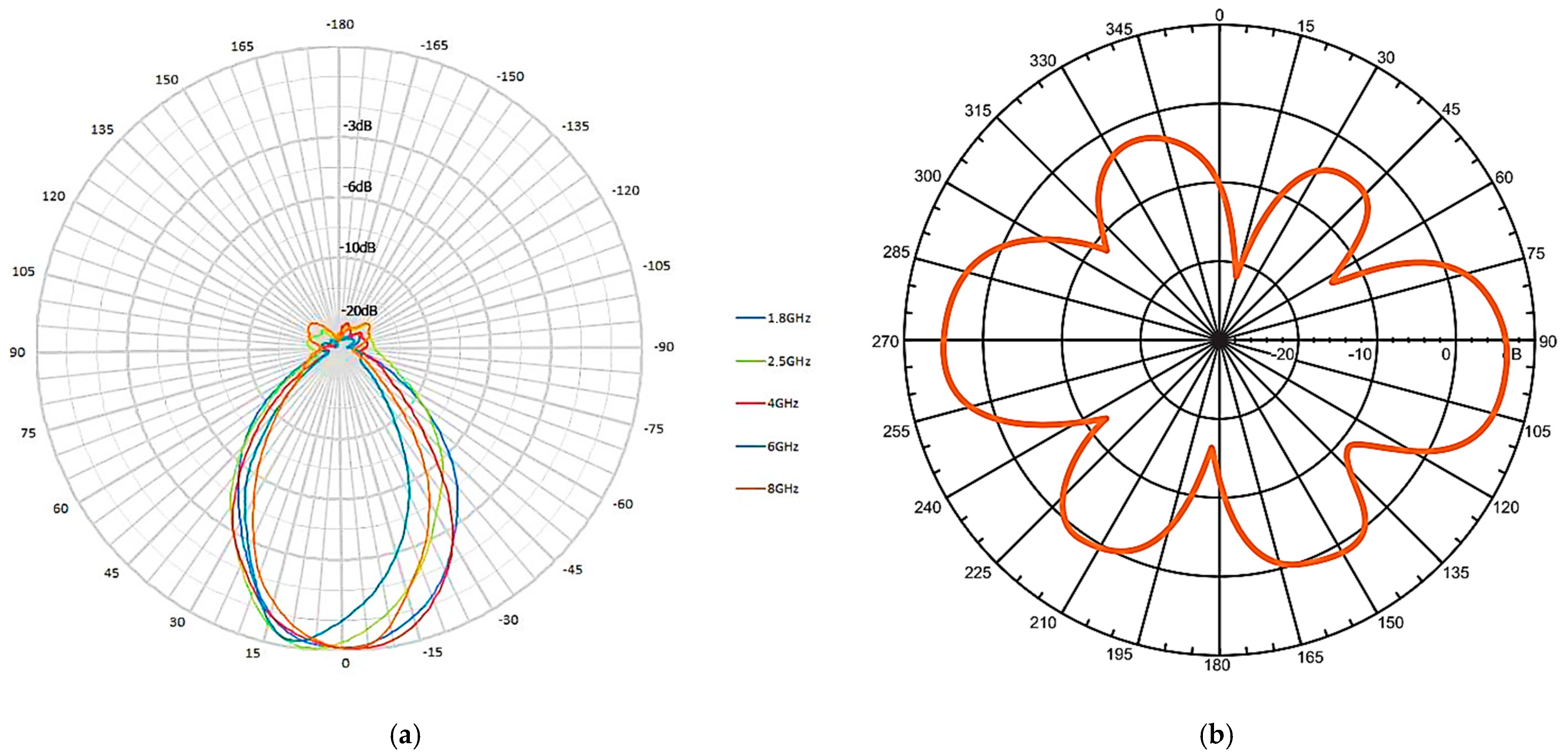
The transmitting and receiving antennas have a fixed position at a distance of 1.5 m from each other, which at 2.4 GHz is greater than 10 wavelengths, enabling far-field measurements to be performed. Both antennas presented in Figure 1, the Wi-Fi pigtail and log-periodic receiving antenna, have a vertical polarization, and are directional in the vertical plane. The transmitting router uses a TP-LINK RP-SMA 2.4 GHz Wi-Fi antenna, model TL-ANT2405CL, with a 5 dBi gain. On the receiver side, the Aaronia HyperLOG 60100 has a gain of 5 to 6 dBi in its entire operating frequency range, from 0.68 to 10 GHz. The radiation patterns for the two antennas are presented in Figure 2. According to their corresponding manufacturers, both antennas have a beamwidth of about 50 degrees at −3 dB or half power, at 2.4–2.5 GHz. The shielded room prevents any unwanted signals from the outside to interfere with the Wi-Fi transmission. The devices and antennas used for the experimental setup are placed on wooden tables, that will not reflect the transmitted wave. This results in a line-of-sight transmission, with no fading.
The APTF and APDP were implemented in order to evaluate the measured Wi-Fi signal’s stationarity. Multiple sliding window sizes and frequency/time deviations were tested when computing the correlation vectors. Depending on the size of the dataset, the sliding window varied from 10 samples to about 10% of the dataset size. The offset between each vector pair, required to compute the correlations, varied from about 10% to 80% of the dataset size. In each case, the allowance of similarity level was analyzed. The case in which the correlation vector had the highest ASL was considered optimal with respect to the chosen sliding window and offset (time delay or frequency deviation) sizes. The stationarity intervals as well as the optimal values for the sliding window sizes were also determined for each measured Wi-Fi dataset.

4. Results

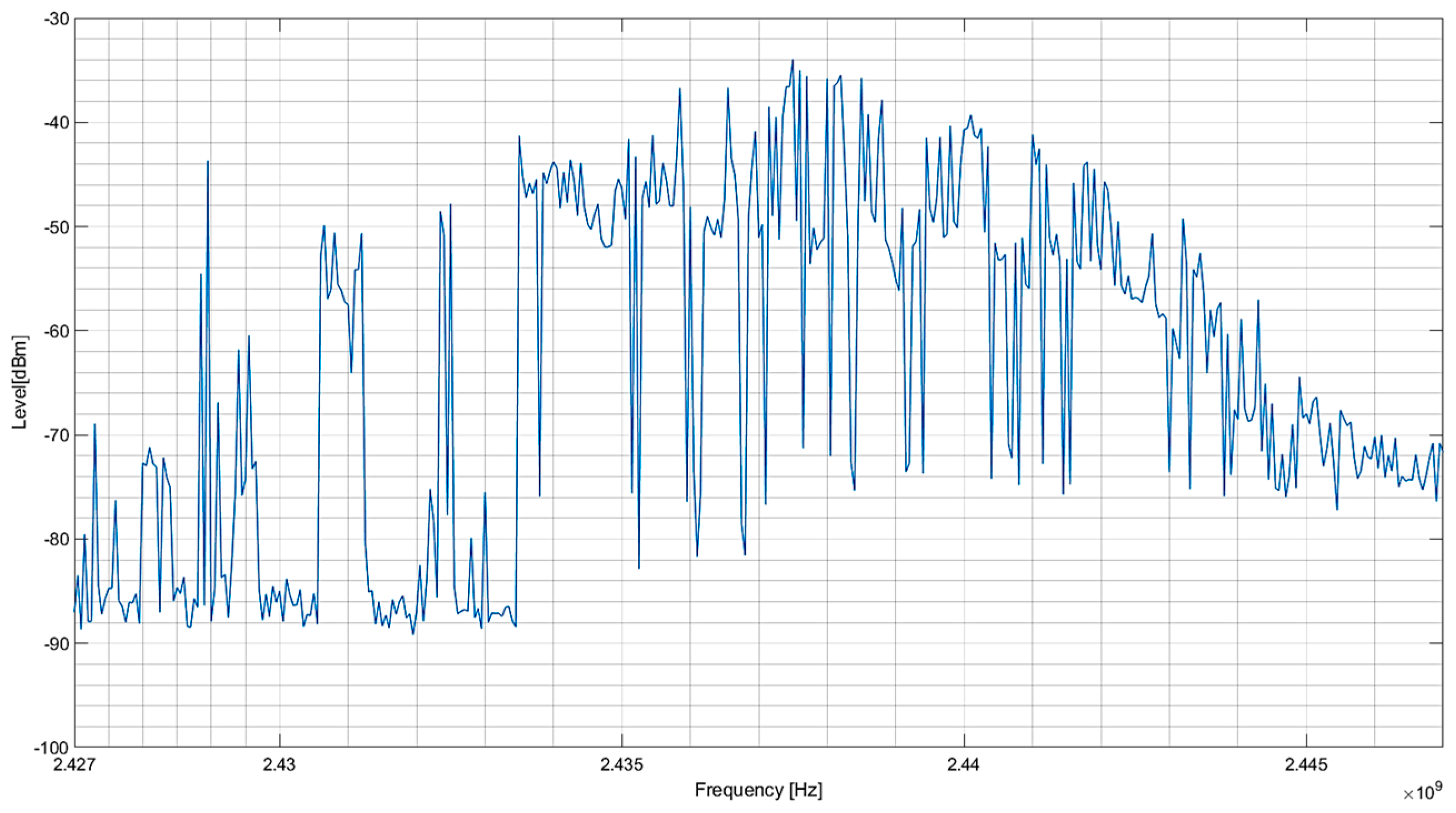
For a comprehensive analysis of the signal variability, the measurement apparatus was configured to record signals within a specific frequency band over a designated time span. Figure 3 illustrates a typical power spectral density (PSD) for emissions from the streaming video data. A noteworthy field level increase of about 50 dB is observed when compared to the scenario without streaming.
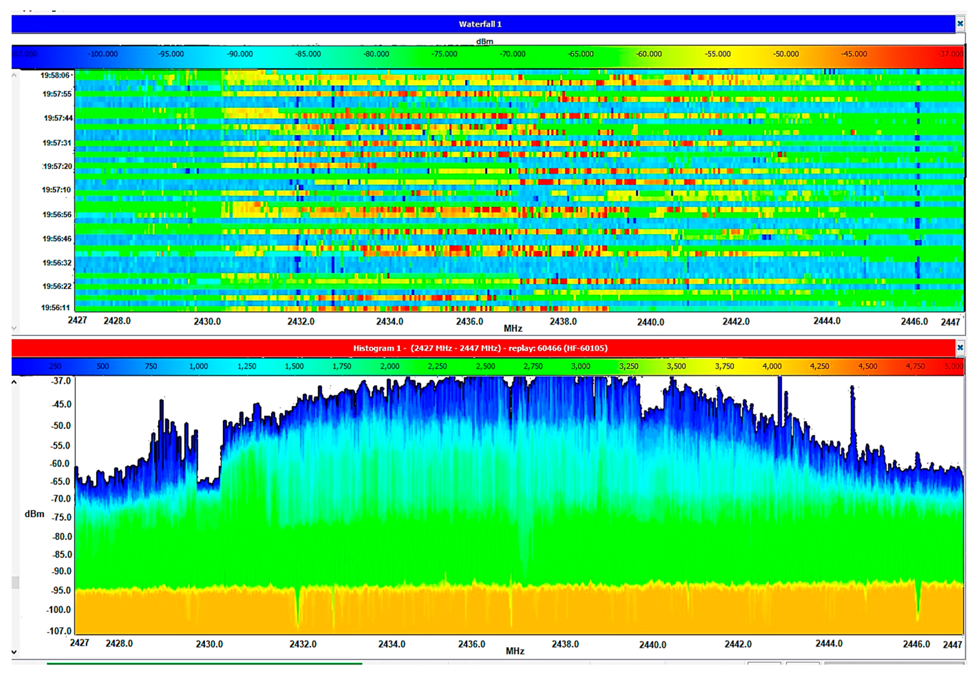
In order to depict in Figure 4 the time variation of the PSD within the designated channel, two illustrations are employed: the waterfall in the upper side, and the persistence representation in the lower side, respectively.
As discerned from the measurements, Wi-Fi signals consistently manifest fluctuations in their frequency content over time. Conventional time-domain or frequency-domain representations may inadequately capture these dynamic characteristics. The waterfall representation, characterized by its time–frequency plot, furnishes a more encompassing perspective on the temporal evolution of the signal’s frequency content. The power level corresponding to each spectral component is illustrated by a color code represented in the upper part of the graph, the x-axis represents frequency values, and the y-axis represents the sweep index or measurement time.
Conversely, the representation of spectrum persistence integrates details regarding the enduring presence of spectral characteristics within a signal, elucidating the temporal persistence of diverse frequencies. The frequency values are depicted along the x-axis, while the power level is conveyed along the y-axis. The persistence of frequency components is visually conveyed through a color code situated in the upper segment of the graph. In this color code, higher frequencies on the scale correspond to more frequent repetitions of spectral components in the signal.
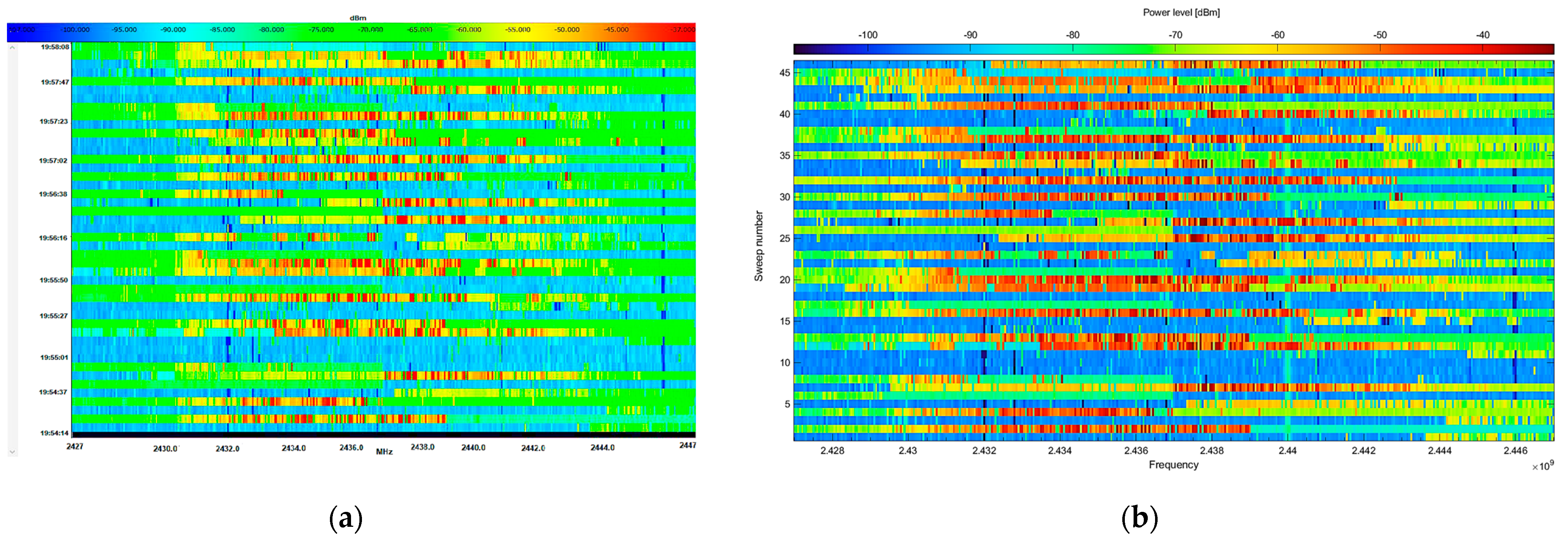
The temporal evolution of power levels within the scrutinized frequency band is visually represented in a waterfall-type display. The recorded data were stored in a file that included discretized frequency band values along with corresponding power levels for each spectral component. Subsequently, the file underwent processing in MATLAB, and the data were formatted for subsequent analyses. Aaronia MCS software (version 2.1.5) produced measurement files in a txt-compatible format, containing various measurement data in addition to frequency and spectral level values. To address this, a MATLAB script was designed to methodically import the entire content of the text file into a character vector. The script then proceeded to ascertain the sequential frequency values, enumerate the sweeps, and identify the initial and final positions for each sweep. Subsequently, the values associated with individual spectral components within each sweep were extracted. Finally, a conversion from string format to double format was implemented for all the extracted values.
In order to verify the precision of this representation, Figure 5 illustrates, for comparative analysis, the cascade representation of a 2-min measurement sequence within the frequency band of 2427–2447 MHz. This representation is generated both by using Aaronia MCS software—on the left side—and with MATLAB—utilizing the recorded data and the imagesc function—on the right side, respectively. The juxtaposition of the two images serves to illustrate that the processing of the recording file in MATLAB aptly extracted pertinent data pertaining to the temporal variations in the spectral content of the signal.
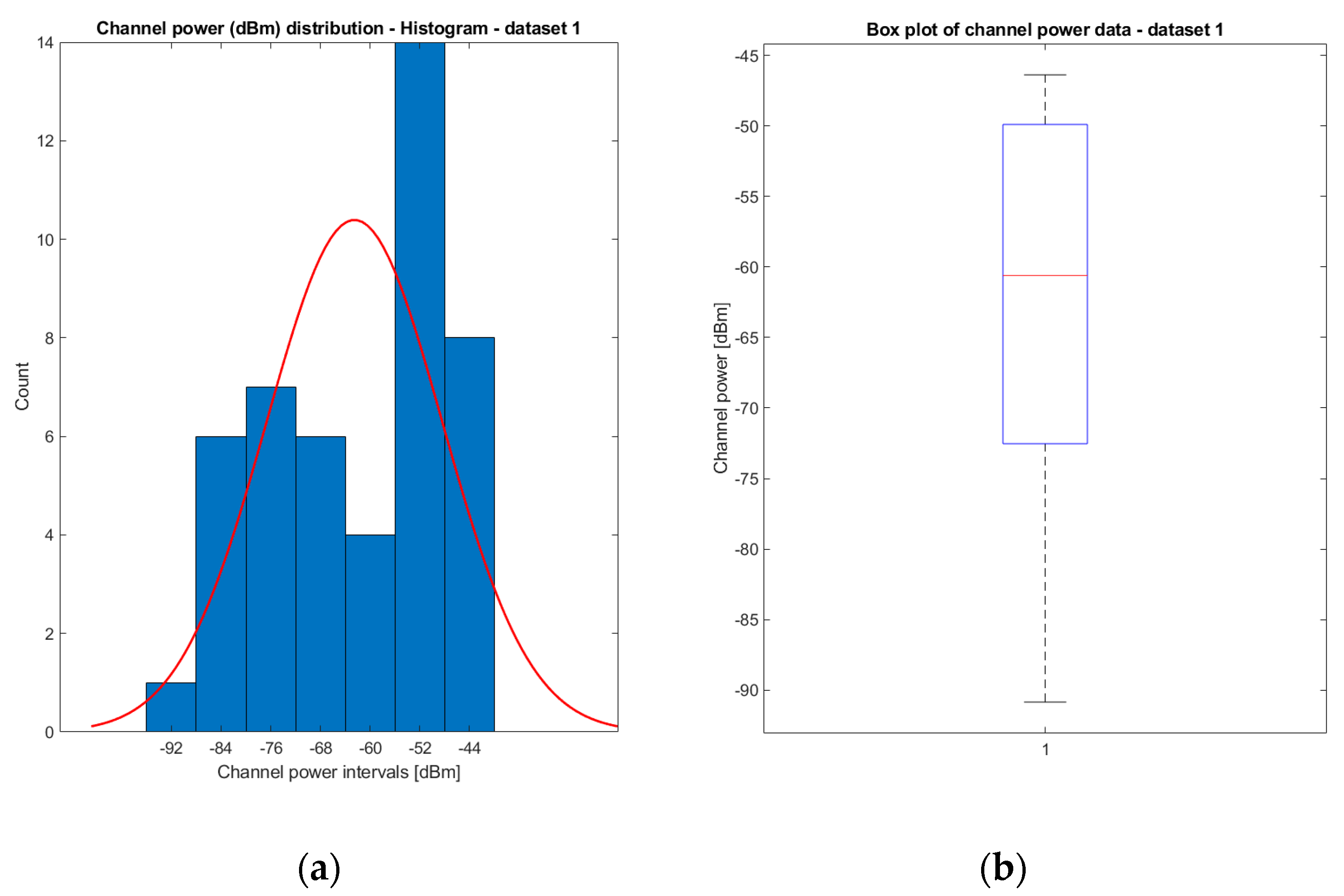
For each frequency sweep, the total channel power is computed using Equation (6). The resulting data, representing the time variation of the total power within the designated Wi-Fi channel, is analyzed by applying descriptive statistics methods. The results are illustrated in Figure 5 and the corresponding parameters are given in Table 1. The histogram also includes a red continuous line representing the Gaussian distribution characterized by the same mean and standard deviation parameters as the dataset.
In order to detect a recognizable pattern of fluctuation in the evolution of the Wi-Fi signal, multiple sets of data were collected through the successive monitoring of Wi-Fi activity. Subsequently, five datasets were chosen for the ensuing analysis based on specific criteria:
  • The initial dataset, denoted as dataset 1, served as the reference for measurements. It was recorded for a brief duration of 2 min while the Wi-Fi source continuously streamed video data on a specific 20 MHz bandwidth channel.
  • Datasets 2_1 and 2_2 were captured over an extended time frame of 25 and 30 min, respectively, while maintaining the same bandwidth.
  • The third set of measurements resulted in datasets 3_1 and 3_2, expanding the analysis further. Dataset 3_1 had a duration of 60 min, while dataset 3_2 covered an extended frequency band ranging from 2.4 GHz to 2.5 GHz within a constrained temporal duration of 7.5 min.
For each frequency sweep of the designated bandwidth, the channel power was computed. Table 1 provides the main parameters and descriptive statistics of channel power variation for these datasets.
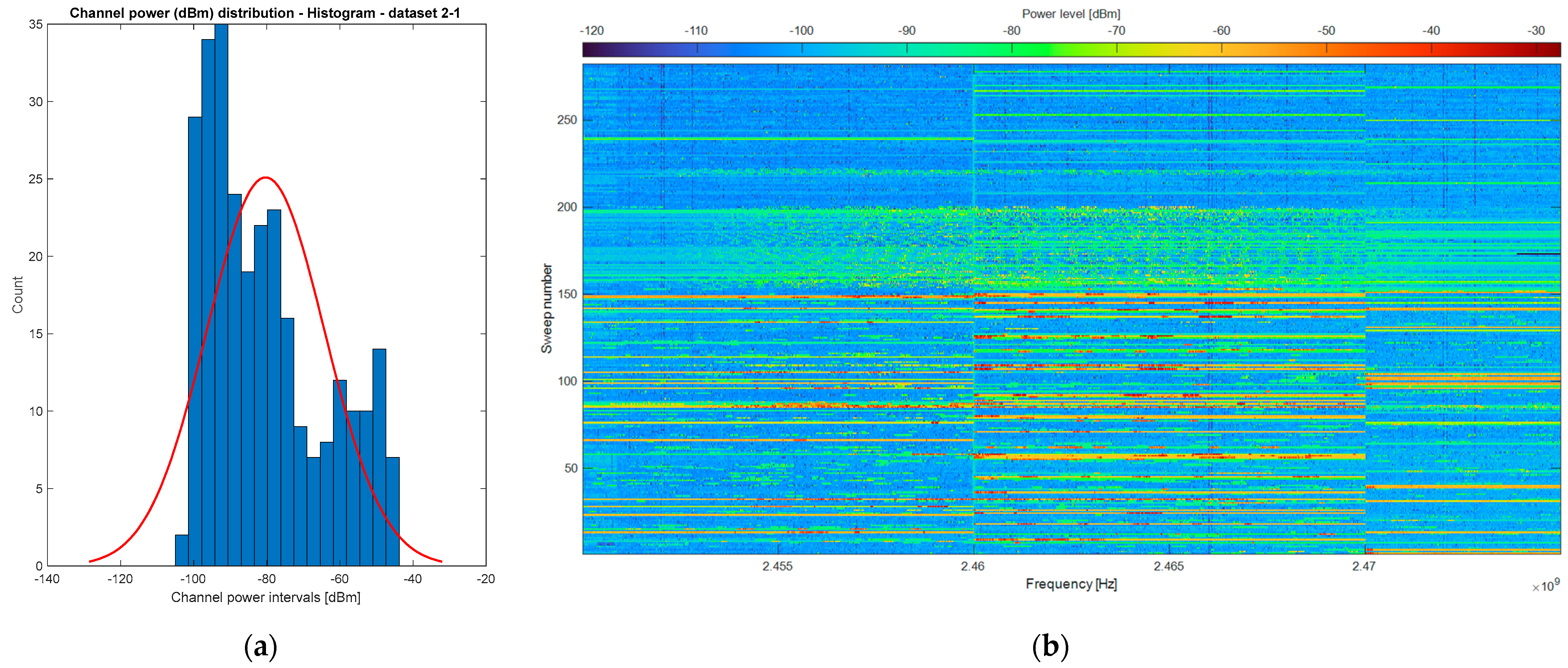
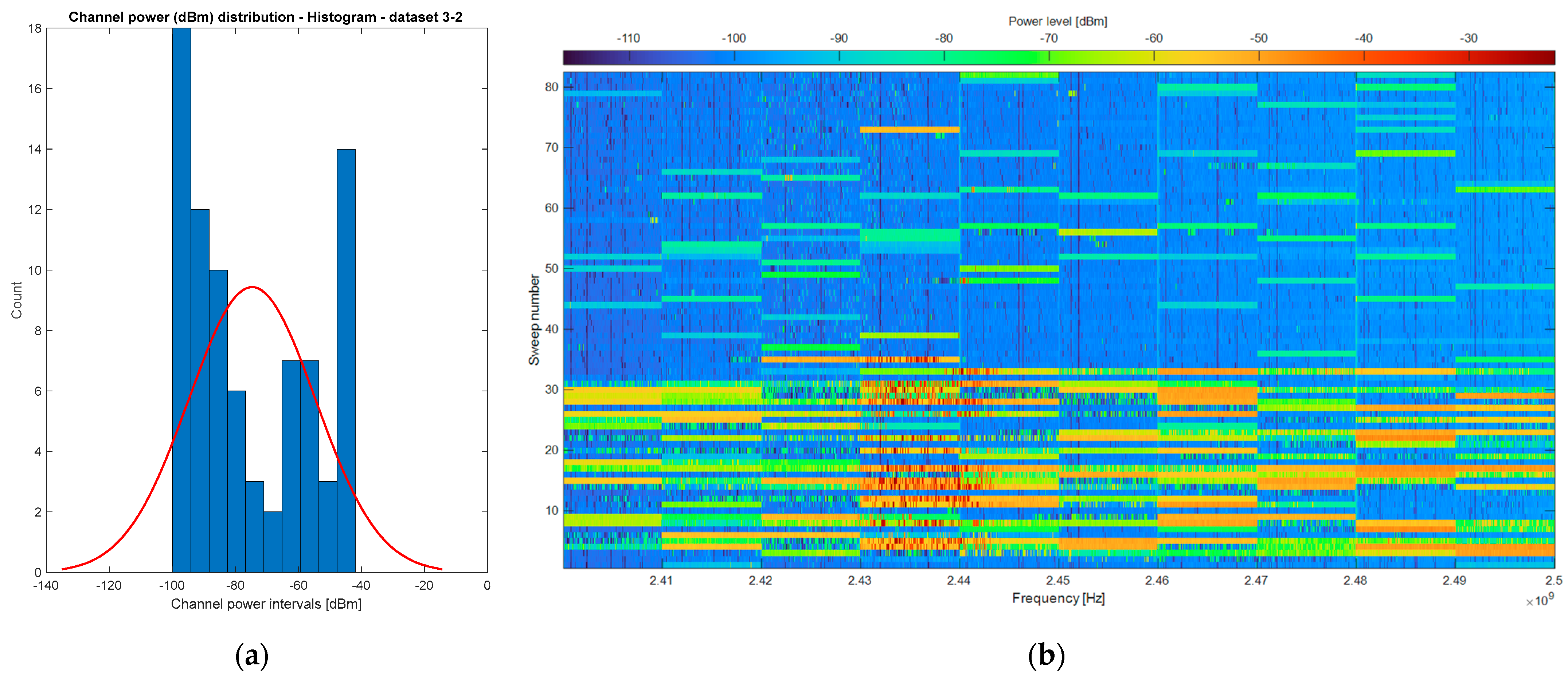
The channel power distribution, depicted in histogram form, was undertaken for all datasets. Figure 6 presents this distribution for the initial dataset, while Figure 7, Figure 8, Figure 9 and Figure 10 display the corresponding histograms for the subsequent datasets.
Every histogram depiction of the datasets additionally incorporates a visual representation of the Gaussian distribution characterized by the same mean and standard deviation parameters corresponding to the respective dataset. Concurrently, the temporal evolution of the spectrum is visually represented in a waterfall format alongside the histograms in Figure 7, Figure 8, Figure 9 and Figure 10.

5. Discussion

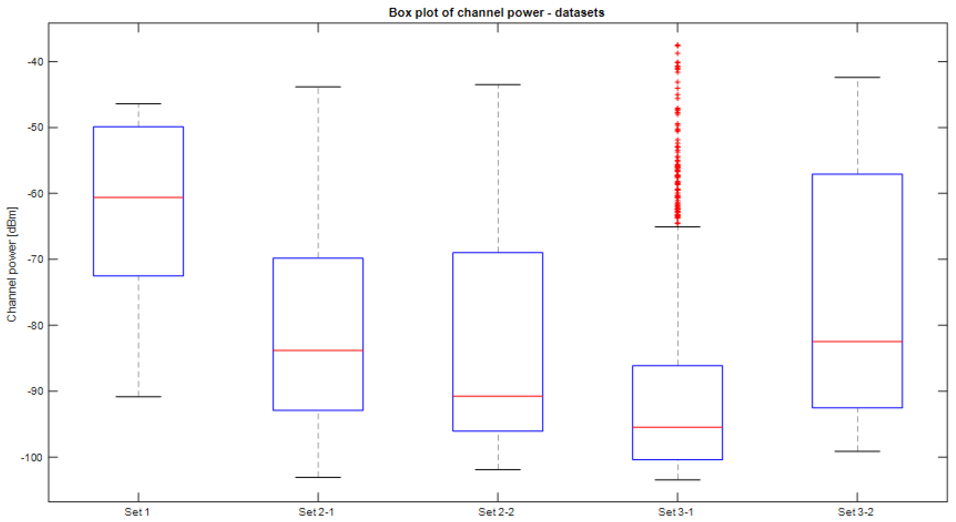
In order to identify a discernible pattern of fluctuation in the signal evolution within a Wi-Fi channel, multiple datasets were amassed, each spanning durations surpassing those of the initial dataset. Subsequently, to ascertain the recurrence of spectrum variability on broader scales, the frequency band was expanded for the final dataset, denoted as 3_2. The duration and recording band parameters were varied precisely to identify their impacts on the statistical parameters. To offer a unified perspective on the temporal variation of channel power across all datasets, two metrics are utilized: the boxplot representation and the cumulative distribution. The boxplot is a statistical visualization summarizing the distribution of a dataset, including the median—red line, the quartiles—blue box, and potential outliers—red points. Figure 11 presents a consolidated depiction of the boxplot representation illustrating the variation in channel power across all datasets.
The CDF is a statistical tool that illustrates the cumulative probability distribution of a random variable. It calculates the cumulative probabilities by assessing the proportion of data points less than or equal to each value in the dataset. This information is graphically represented, revealing the progressive accumulation of probabilities as values increase. Figure 12 illustrates the CDFs for all datasets.
Stationarity analysis, using the APTF and APDP methods, was also performed on the measured Wi-Fi datasets presented in Table 1. For each dataset, we determined the allowance of similarity level, as well as average correlation values, computed for fixed (optimal) window lengths but different correlation offsets: time delays for APDP or frequency deviations for APTF. A general correlation average was also computed for each dataset, regardless of sliding window or offset lengths. These results are presented in Table 2.
The results show a low or insignificant correlation. The only dataset that could be considered for potential stationarity is the first. This dataset corresponds to the shortest Wi-Fi measurement (2 min), which indicates that longer exposure times, comparable to the other datasets, may require stationarity analysis.
Table 3 presents the optimal values that enable the highest allowance of similarity level for each dataset. It is worth noting that without real-time frequency measurements, the stationary time interval can only be determined based on spectrum analyzer sweep time. This limits the APDP algorithm’s capacity for precise stationarity evaluation.
Figure 13 and Figure 14 present the correlation results yielded by the APTF and APDP algorithms. The correlation coefficients generally vary between 0.1 and 0.5, indicating a low correlation. It is also worth noting that for dataset 3.2, any multiple of 10 MHz could have a good value to enable a high allowance of similarity, though 50 MHz was chosen as it yields the greatest average correlation.
Though the minimum and average correlation values are similar to the APTF results, there are instances, especially for longer exposure datasets like 3.1, where correlation values close to unitary are achieved.
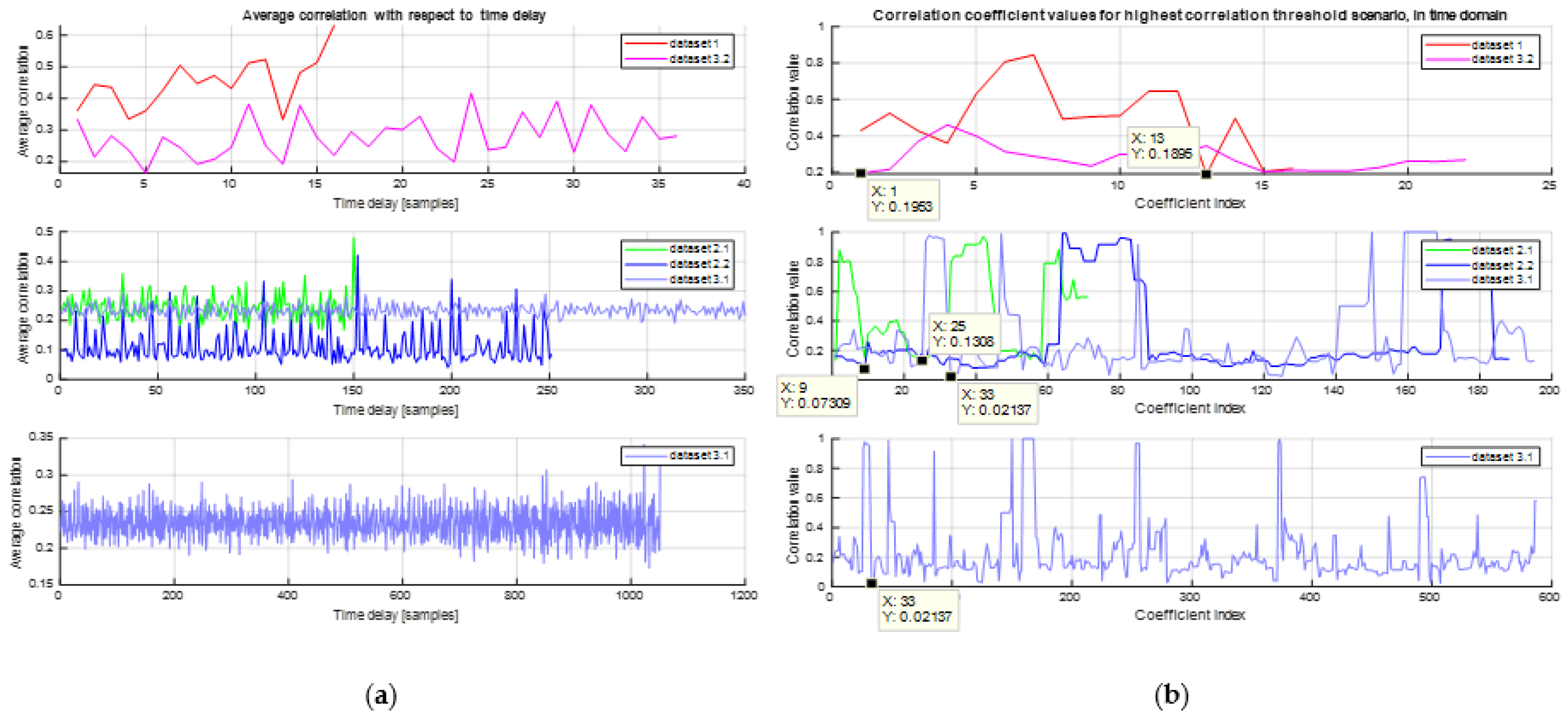
According to Equation (16), each frequency deviation Δf will yield a different correlation coefficient vector. The Average correlation presented in Figure 13a is the mean computed for each of these vectors, each corresponding to a different Δf. Figure 13b presents the correlation coefficient vectors for fixed Δf values, one for each dataset, which are presented in Table 3.
These fixed values for Δf are the ones that yield the highest allowance of similarity level (CASL), as mentioned in Equations (13) and (17). In other words, out of all simulations performed in MATLAB, the correlation vectors corresponding to these fixed frequency deviations have the greatest minimum value.
Out of all frequency deviations Δf for which the corresponding correlation values overcome this threshold, the greatest Δf value is retained and becomes the stationarity interval or bandwidth, as suggested in Equation (17).
The determined CASL values, which are presented in Table 2, are also underlined in Figure 13b, using annotations, as the minimum values of the correlation vectors computed for each dataset.
Figure 14 shows that similar results were obtained for the time-domain (APDP) stationarity analysis.
Based on the APTF and APDP analyses, the conclusion is that the measured Wi-Fi signals are not stationary in either time or frequency domains. This result presents an issue regarding the possibility of simulating Wi-Fi signals. It shows that implementing the modulations specific to the 802.11 standards (OFDM and DSSS) [32], even with added Gaussian noise, may not be enough if you want to simulate a real Wi-Fi signal.
Based on the five datasets’ average statistical parameters, we generated multiple discrete frequency domain signals that would correspond to a real Wi-Fi signal, measured with a spectrum analyzer. The statistical parameters for the five measured datasets are presented in Table 4.
Using these values, we generated random vectors of length 1000 from the Pearson system of distributions. These vectors all have the same mean and variance as the average values computed for the five datasets, while the skewness and kurtosis vary with a maximum of ±5% from the average values presented in Table 5. As these vectors simulate a frequency domain power measurement, the APTF method was used to evaluate their stationarity. The results are presented in Table 5. The ASL is around 0.1, and the average correlation varies between 0.3 and 0.4. The results are similar to the practical datasets regarding both the allowance of similarity level and average correlation.
Programmable devices, such as an SDR or RFSoC, can also be used to generate similar nonstationary Wi-Fi vectors. This can represent a solution for a noncommercial, laboratory Wi-Fi generator, that can be developed to comply to biomedical standards in order to be used in experiments of this nature. The method can be migrated to other technologies and applications, such as LoRa, NB-IoT, or BLE. From a mobile standpoint, any practical implementation should also take into account the antenna orientation and distance to the Wi-Fi transmitter [50], and measurements should be performed accordingly in order to update the statistical parameters of the generated Wi-Fi signals.

6. Conclusions

The stationarity of electromagnetic emission sources, particularly those generating time-varying EMFs, can significantly impact living organisms. Exposure to nonstationary sources with dynamic signals limits an organism’s ability to adapt to the changing stimulus. The consideration that real-life source signals may be more biologically active raises concerns about the accuracy and relevance of laboratory sources in experiments studying the effects of RF-EMF exposure. However, using real-life sources with unpredictable variations contradicts the principle of experiment controllability. The investigation into the impact of Wi-Fi routers on living organisms is crucial, as these emission sources exhibit either weak stationarity or nonstationarity, potentially leading to adverse effects on human health.
The paper describes the examination of temporal variations in ambient electromagnetic exposure emanating from Wi-Fi communication devices which involves the application of diverse statistical methodologies. The objective is to ascertain the stationarity of these signals. The ultimate outcome aims to produce laboratory-controlled signals that faithfully replicate the authentic variability observed in real-life signals generated by Wi-Fi communication devices.
Several datasets were obtained from various frequency-domain measurements with a spectrum analyzer. A stationarity analysis was performed for the measured datasets, in both time and frequency domains, using the ADPD and APTF methods.
The findings derived from the analysis using APTF and APDP indicate that the observed Wi-Fi signals lack stationarity in both the time and frequency domains. This outcome poses a challenge with respect to simulating Wi-Fi signals, suggesting that the incorporation of modulations exclusive to the 802.11 standards (OFDM and DSSS), along with the introduction of Gaussian noise, may prove insufficient for an accurate emulation of authentic Wi-Fi signals.
We suggest, in this case, simulating the spectrum analyzer measurement by generating vectors from the Pearson system of distributions, with statistical parameters that correspond to practical measurements. The quality of these simulated Wi-Fi waveforms will depend on the measurements used to train the algorithm. These waveforms could be used for further EMF investigation by generating them using a portable SDR device, without requiring a Wi-Fi router with Internet access.

Author Contributions

Conceptualization, G.R. and L.T.; methodology, G.R.; software, L.T.; validation, G.R., L.T. and A.A.; formal analysis, L.T.; investigation, S.S.-D.; resources, L.O.F.; data curation, L.T.; writing—original draft preparation, G.R. and L.T.; writing—review and editing, G.R.; visualization, L.T.; supervision, G.R. and L.O.F.; project administration, G.R. and S.S.-D.; funding acquisition, G.R. and S.S.-D. All authors have read and agreed to the published version of the manuscript.

Funding

This research was funded by the Helmut Schmidt University.

Data Availability Statement

The data presented in this study are available upon request from the corresponding author.

Conflicts of Interest

The authors declare no conflicts of interest.

References

  1. Gajšek, P.; Ravazzani, P.; Wiart, J.; Grellier, J.; Samaras, T.; Thuróczy, G. Electromagnetic field exposure assessment in Europe radiofrequency fields (10 MHz–6 GHz). J. Expo. Sci. Environ. Epidemiol. 2015, 25, 37–44. [Google Scholar] [CrossRef] [PubMed]
  2. Atanasova, G.; Atanasov, B.; Atanasov, N. Assessment of Electromagnetic Field Exposure on European Roads: A Comprehensive In Situ Measurement Campaign. Sensors 2023, 23, 6050. [Google Scholar] [CrossRef] [PubMed]
  3. Urbinello, D.; Joseph, W.; Verloock, L.; Martens, L.; Röösli, M. Temporal trends of radio-frequency electromagnetic field (RF-EMF) exposure in everyday environments across European cities. Environ. Res. 2014, 134, 134–142. [Google Scholar] [CrossRef] [PubMed]
  4. Sârbu, A.; Miclău, S.; Digulescu, A.; Bechet, P. Comparative Analysis of User Exposure to the Electromagnetic Radiation Emitted by the Fourth and Fifth Generations of Wi-Fi Communication Devices. Int. J. Environ. Res. Public. Health 2020, 17, 8837. [Google Scholar] [CrossRef] [PubMed]
  5. Mulugeta, B.; Wang, S.; Chikha, W.B.; Liu, J.; Roblin, C.; Wiart, J. Statistical Characterization and Modeling of Indoor RF-EMF Down-Link Exposure. Sensors 2023, 23, 3583. [Google Scholar] [CrossRef] [PubMed]
  6. Bonato, M.; Dossi, L.; Chiaramello, E.; Fiocchi, S.; Tognola, G.; Parazzini, M. Stochastic Dosimetry Assessment of the Human RF-EMF Exposure to 3D Beamforming Antennas in indoor 5G Networks. Appl. Sci. 2021, 11, 1751. [Google Scholar] [CrossRef]
  7. European Council. Recommendation of 1999 on the Limitation of Exposure of the General Public to Electromagnetic Fields (0 Hz to 300 GHz). Off. J. Eur. Communities L1999/519/EC 1999, 199, 59–70. [Google Scholar]
  8. European Union. Directive 2014/30/EU of the European Parliament and of the Council. Off. J. Eur. Union 2014, 96, 79. [Google Scholar]
  9. Redmayne, M.; Maisch, D. ICNIRP Guidelines’ Exposure Assessment Method for 5G Millimetre Wave Radiation May Trigger Adverse Effects. Int. J. Environ. Res. Public. Health 2023, 20, 5267. [Google Scholar] [CrossRef]
  10. Chou, C.-K. Controversy in Electromagnetic Safety. Int. J. Environ. Res. Public. Health 2022, 19, 16942. [Google Scholar] [CrossRef]
  11. Bas, O.; Sengul, I.; Bas, O.; Hanci, H.; Degermenci, M.; Sengul, D.; Altuntas, E.; Soztanaci, U.; Sonmez, O.S.J.J. Impressions of the chronic 900-MHz electromagnetic field in the prenatal period on Purkinje cells in male rat pup cerebella: Is it worth mentioning? Rev. Assoc. Med. Bras. (1992) 2022, 68, 1383–1388. [Google Scholar] [CrossRef] [PubMed]
  12. Cantürk, T.F.; Yalçin, B.; Yay, A.; Tan, B.; Yeğin, K.; Daşdağ, S. Effects of pre and postnatal 2450 MHz continuous wave (CW) radiofrequency radiation on thymus: Four generation exposure. Electromagn. Biol. Med. 2022, 41, 315–324. [Google Scholar] [CrossRef] [PubMed]
  13. Er, H.; Tas, G.; Soygur, B.; Ozen, S.; Sati, L. Acute and Chronic Exposure to 900 MHz Radio Frequency Radiation Activates p38/JNK-mediated MAPK Pathway in Rat Testis. Reprod. Sci. 2022, 29, 1471–1485. [Google Scholar] [CrossRef] [PubMed]
  14. Gupta, S.; Patel, S.; Tomar, M.; Singh, S.; Mesharam, M.; Krishnamurthy, S. Long-term exposure of 2450 MHz electromagnetic radiation induces stress and anxiety like behavior in rats. Neurochem Int. 2019, 128, 1–13. [Google Scholar] [CrossRef] [PubMed]
  15. National Toxicology Program. NTP TR 596 Technical Report on the Toxicology and Carcinogenesis Studies in B6C3F1/N Mice Exposed to Whole-Body Radio Frequency Radiation at a Frequency (1900 MHz) and Modulations (GSM and CDMA) Used by Cell Phones; U.S. Department of Health and Human Services: Research Triangle Park, NC, USA, 2018.
  16. Qin, F.; Cao, H.; Yuan, H.; Guo, W.; Pei, H.; Cao, Y.; Tong, J. 1800 MHz radiofrequency fields inhibits testosterone production via CaMKI/RORα pathway. Reprod. Toxicol. 2018, 81, 229–236. [Google Scholar] [CrossRef] [PubMed]
  17. Rui, G.; Liu, L.; Guo, L.; Xue, Y.; Lai, P.; Gao, P.; Xing, J.; Li, J.; Ding, G. Effects of 5.8 GHz microwave on hippocampal synaptic plasticity of rats. Int. J. Environ. Health Res. 2022, 32, 2247–2259. [Google Scholar] [CrossRef] [PubMed]
  18. Souffi, S.; Lameth, J.; Gaucher, Q.; Arnaud-Cormos, D.; Lévêque, P.; Edeline, J.-M.; Mallat, M. Exposure to 1800 MHz LTE electromagnetic fields under proinflammatory conditions decreases the response strength and increases the acoustic threshold of auditory cortical neurons. Sci. Rep. 2022, 12, 4063. [Google Scholar] [CrossRef]
  19. Xue, Y.; Guo, L.; Lin, J.; Lai, P.; Rui, G.; Liu, L.; Huang, R.; Jing, Y.; Wang, F.; Ding, G. Effects of 5.8 GHz Microwaves on Testicular Structure and Function in Rats. BioMed Res. Int. 2022, 2022, 5182172. [Google Scholar] [CrossRef]
  20. Panagopoulos, D. Analyzing the Health Impacts of Modern Telecommunications Microwaves. In Advances in Medicine and Biology Volume 17; Nova Science Publishers, Inc.: Hauppauge, NY, USA, 2011; pp. 1–55. [Google Scholar]
  21. Tsatsakis, A.; Kouretas, D.; Tzatzarakis, M.; Stivaktakis, P.; Tsarouhas, K.; Golokhvast, K.; Rakitskii, V.; Tutelyan, V.; Hernandez, A.; Rezaee, R.; et al. Simulating real-life exposures to uncover possible risks to human health: A proposed consensus for a novel methodological approach. Hum. Exp. Toxicol. 2017, 36, 554–564. [Google Scholar] [CrossRef]
  22. Rowley, J.; Joyner, K. Comparative international analysis of radiofrequency exposure surveys of mobile communication radio base stations. J. Expo. Sci. Environ. Epidemiol. 2012, 22, 304–315. [Google Scholar] [CrossRef]
  23. Bartosova, K.; Neruda, M.; Vojtech, L. Methodology of Studying Effects of Mobile Phone Radiation on Organisms: Technical Aspects. Int. J. Environ. Res. Public. Health 2021, 18, 12642. [Google Scholar] [CrossRef] [PubMed]
  24. Kostoff, R.N.; Heroux, P.; Aschner, M.; Tsatsakis, A. Adverse health effects of 5G mobile networking technology under real-life conditions. Toxicol. Lett. 2020, 323, 35–40. [Google Scholar] [CrossRef]
  25. Sienkiewicz, Z.; Calderón, C.; Broom, K.; Addison, D.; Gavard, A.; Lundberg, L.; Maslanyj, M. Are Exposures to Multiple Frequencies the Key to Future Radiofrequency Research? Front. Public Health 2017, 5, 328. [Google Scholar] [CrossRef] [PubMed]
  26. Miclaus, S.; Bechet, P.; Iftode, C. The application of a channel-individualized method for assessing long-term, realistic exposure to radiofrequency radiation emitted by mobile communication base station antennas. Measurement 2013, 46, 1355–1362. [Google Scholar] [CrossRef]
  27. Panagopoulos, D.J.; Johansson, O.; Carlo, G.L. Real versus Simulated Mobile Phone Exposures in Experimental Studies. BioMed Res. Int. 2015, 2015, 607053. [Google Scholar] [CrossRef] [PubMed]
  28. Modell, H.; Cliff, W.; Michael, J.; McFarland, J.; Wenderoth, M.; Wright, A. A physiologist’s view of homeostasis. Adv. Physiol. Educ. 2015, 39, 259–266. [Google Scholar] [CrossRef] [PubMed]
  29. Vodovotz, Y.; An, G.; Androulakis, I. A systems engineering perspective on homeostasis and disease. Front. Bioeng. Biotechnol. 2013, 1, 6. [Google Scholar] [CrossRef]
  30. Roşu, G.; Spandole-Dinu, S.; Catrina, A.-M.; Tuţă, L.; Baltag, O.; Fichte, L.-O. On the adapting ability of living organisms to stationary and non-stationary electromagnetic fields. IOP Conf. Ser. Mater. Sci. Eng. 2022, 1254, 012024. [Google Scholar] [CrossRef]
  31. Rust, H. Spectral Analysis of Stochastic Processes; E2C2/GIACS Summer School: Comorova, Romania, 2007. [Google Scholar]
  32. IEEE-SA. The Evolution of Wi-Fi Technology and Standards. 16 May 2023. Available online: https://standards.ieee.org/beyond-standards/the-evolution-of-wi-fi-technology-and-standards/ (accessed on 10 November 2023).
  33. Papoulis, A.; Pillai, S.U. Probability, Random Variables, and Stochastic Processes; McGraw-Hill Higher Education: New York, NY, USA, 2002. [Google Scholar]
  34. Tan, Y.; Wang, C.-X.; Nielsen, J.Ø.; Pedersen, G.F. Comparison of stationarity regions for wireless channels from 2 GHz to 30 GHz. In Proceedings of the 2017 13th International Wireless Communications and Mobile Computing Conference (IWCMC), Valencia, Spain, 26–30 June 2017; pp. 647–652. [Google Scholar] [CrossRef]
  35. Spandole-Dinu, S.; Catrina, A.-M.; Voinea, O.; Andone, A.; Radu, S.; Haidoiu, C.; Călborean, O.; Popescu, D.; Suhăianu, V.; Baltag, O.; et al. Pilot Study of the Long-Term Effects of Radiofrequency Electromagnetic Radiation Exposure on the Mouse Brain. Int. J. Environ. Res. Public. Health 2023, 20, 3025. [Google Scholar] [CrossRef]
  36. IEEE Computer Society. IEEE Std 802.11™ IEEE Standard for Information Technology, Part 11: Wireless LAN Medium Access Control; The Institute of Electrical and Electronics Engineers: New York, NY, USA, 2021; ISBN 9781504472838/9781504472845. [Google Scholar]
  37. Banerji, S.; Chowdhury, R.S. On IEEE 802.11: Wireless LAN Technology. Int. J. Mob. Netw. Commun. Telemat. (IJMNCT) 2013, 3, 45–64. [Google Scholar] [CrossRef]
  38. Tardioli, D.; Almeida, L. Behavior of IEEE 802.11 devices under interference. In Proceedings of the IEEE 28th International Conference on Emerging Technologies and Factory Automation (ETFA), Sinaia, Romania, 12–15 September 2023. [Google Scholar] [CrossRef]
  39. Kostuch, A.; Gierłowski, K.; Wozniak, J. Performance Analysis of Multicast Video Streaming in IEEE 802.11 b/g/n Testbed Environment. In Proceedings of the IFIP International Federation for Information Processing, Gdańsk, Poland, 9–11 September 2009; pp. 92–105. [Google Scholar]
  40. Rosu, G.; Tuta, L.; Halca, A.; Bicheru, S.; Hertzog, R.; Baltag, O. Experimental Platform for Studying the Impact of Environ-mental Electromagnetic Fields on Living Organisms. In Proceedings of the 13th International Conference on Communications (COMM), Bucharest, Romania, 18–20 June 2020. [Google Scholar]
  41. Narasimhamurthy, A.B.; Banavar, M.K.; Tepedelenlioğlu, C. Peak to Average Power Ratio. In OFDM Systems for Wireless Communications; Springer Nature: Cham, Switzerland, 2010; pp. 31–32. [Google Scholar]
  42. Pisa, S.; Pittella, E.; Piuzzi, E. A survey of radar systems for medical applications. IEEE Aerosp. Electron. Syst. Mag. 2016, 31, 64–81. [Google Scholar] [CrossRef]
  43. Joseph, W.; Pareit, D.; Vermeeren, G.; Naudts, D.; Verloock, L.; Martens, L.; Moerman, I. Determination of the duty cycle of WLAN for realistic radio frequency electromagnetic field exposure assessment. Prog. Biophys. Mol. Biology. 2013, 111, 30–36. [Google Scholar] [CrossRef] [PubMed]
  44. Technologies, A. Characterizing Digitally Modulated Signals with CCDF Curves. Application Note; Agilent Technologies: Santa Clara, CA, USA, 2000. [Google Scholar]
  45. Champagnat, N.; Villemonais, D. General criteria for the study of quasi-stationarity. Electron. J. Probab. 2023, 28, 1–84. [Google Scholar] [CrossRef]
  46. Sunao, R.; Satoru, A. Development of Multi-channel APD (Amplitude Probability Distribution) Measuring Apparatus. Anritsu Tech. Rev. 2013, 20, 42–52. [Google Scholar]
  47. Stoica, P.; Moses, R. Spectral Analysis of Signals; Prentice Hall: Hoboken, NJ, USA, 2005. [Google Scholar]
  48. Tognola, G.; Plets, D.; Chiaramello, E.; Gallucci, S.; Bonato, M.; Fiocchi, S.; Parazzini, M.; Martens, L.; Joseph, W.; Ravazzani, P. Use of Machine Learning for the Estimation of Down- and Up-Link Field Exposure in Multi-Source Indoor WiFi Scenarios. Bioelectromagnetics 2021, 42, 550–561. [Google Scholar] [CrossRef] [PubMed]
  49. Rauscher, C. Fundamentals of Spectrum Analysis; Rohde & Schwarz GmbH: München, Germany, 2001. [Google Scholar]
  50. Miclaus, S.; Deaconescu, D.; Vatamanu, D.; Buda, A. An Exposimetric Electromagnetic Comparison of Mobile Phone Emissions: 5G versus 4G Signals Analyses by Means of Statistics and Convolutional Neural Networks Classification. Technologies 2023, 11, 113. [Google Scholar] [CrossRef]
Figure 1. Experimental setup schematic.
Electronics 13 00301 g001
Figure 2. Radiation patterns for the transmitting and receiving antennas presented in Figure 1 (vertical plane), according to the manufacturers’ datasheets: (a) Aaronia HyperLOG 60xx Series; (b) TP-LINK TL-ANT2405CL pigtail antenna.
Electronics 13 00301 g002
Figure 3. Typical spectral distribution for video data streaming.
Electronics 13 00301 g003
Figure 4. Time variation of the power spectral distribution in the designated channel: waterfall (upper side) and persistence (lower side).
Electronics 13 00301 g004
Figure 5. Waterfall representation of the Wi-Fi transmitted signal: first dataset, duration 2 min. (a) View on the spectrum analyzer software; (b) generated using MATLAB processing of the measured data.
Electronics 13 00301 g005
Figure 6. Statistical analysis on the time variation of the total power within the designated channel: first dataset, duration 2 min. (a) Histogram; (b) boxplot.
Electronics 13 00301 g006
Figure 7. Dataset 2_1. (a) Histogram representation of channel power distribution; (b) waterfall visualization of the temporal fluctuations in the spectrum.
Electronics 13 00301 g007
Figure 8. Dataset 2_2. (a) Histogram representation of channel power distribution; (b) waterfall visualization of the temporal fluctuations in the spectrum.
Electronics 13 00301 g008
Figure 9. Dataset 3_1. (a) Histogram representation of channel power distribution; (b) waterfall visualization of the temporal fluctuations in the spectrum.
Electronics 13 00301 g009
Figure 10. Dataset 3_2. (a) Histogram representation of channel power distribution; (b) waterfall visualization of the temporal fluctuations in the spectrum.
Electronics 13 00301 g010
Figure 11. Boxplot distribution of all datasets.
Electronics 13 00301 g011
Figure 12. Cumulative distribution functions of all datasets.
Electronics 13 00301 g012
Figure 13. APTF results for frequency domain stationarity analysis. (a) Correlation with respect to frequency offset; (b) correlation coefficient vectors for highest allowance of similarity level.
Electronics 13 00301 g013
Figure 14. APDP results for time domain stationarity analysis. (a) Correlation with respect to time offset; (b) correlation coefficient vectors for highest allowance of similarity level.
Electronics 13 00301 g014
Table 1. Comparative results of the measurement datasets and corresponding channel power variation.
DatasetParametersChannel Power (CP) Descriptive Statistics
BandwidthDurationMean [dBm]Standard Deviation [dBm]SkewnessKurtosis
120 MHz2 min−62.523814.1263−0.43331.7261
2_120 MHz25 min−80.322716.07950.67112.2847
2_220 MHz30 min−82.733517.67290.97652.4174
3_120 MHz60 min−91.138312.49921.68365.7821
3_2100 MHz7.5 min−74.729820.10550.41051.6322
Table 2. APTF and APDP results for measured Wi-Fi datasets.
DatasetFrequencyTime
Allowance of Similarity LevelHighest Correlation AverageAverage Correlation (for All Δf and Sliding Window Sizes)Allowance of Similarity LevelHighest Correlation AverageAverage Correlation (for All Δt and Sliding Window Sizes)
10.320.47280.27280.180.63110.3889
2-10.030.32890.16280.130.47950.1507
2-20.30.35370.20.070.42080.1430
3-10.170.41010.22430.020.34210.0686
3-20.030.55250.22280.190.41650.2429
Table 3. Optimal values for highest allowance of similarity level.
DatasetFrequencyTime
Frequency Deviation Δf/Stationary Bandwidth [MHz]Sliding Window Size [MHz]Time Delay Δt/Stationary Interval [s]Sliding Window Size [s]
114.552.3563.613.25
2-114.2052.221055.363.96
2-216.3952.235954.2455.38
3-113.52.451114.910.26
3-250.359.65275.8756.3
Table 4. Statistical parameters for the measured Wi-Fi datasets, in the frequency domain.
DatasetMeanVarianceSkewnessKurtosis
19.6532 × 10−44.6564 × 10−61.91856.8177
2.12.0697 × 10−41.5282 × 10−67.320670.4443
2.22.4991 × 10−42.1950 × 10−68.328396.3299
3.18.9638 × 10−59.3443 × 10−715.8252300.1463
3.24.8693 × 10−48.0357 × 10−63.321413.8578
Average3.9975 × 10−43.4699 × 10−67.342897.5192
Table 5. Statistical parameters and APTF results for the simulated Wi-Fi vectors.
Simulated Wi-Fi Dataset12345678910
Mean3.9975 × 10−4
Variance3.4699 × 10−6
Skewness7.51407.47107.62607.69607.67337.64727.66317.68547.70207.5881
Kurtosis102.194592.776795.609294.212598.417897.920193.575993.820395.657392.6714
Allowance of similarity level0.120.100.090.070.090.090.080.080.080.08
Highest correlation average0.37240.37590.34730.35530.34600.35870.32950.37850.35100.3507
Average correlation0.11600.11090.11250.11100.11380.11510.11300.11020.11100.1116
Disclaimer/Publisher’s Note: The statements, opinions and data contained in all publications are solely those of the individual author(s) and contributor(s) and not of MDPI and/or the editor(s). MDPI and/or the editor(s) disclaim responsibility for any injury to people or property resulting from any ideas, methods, instructions or products referred to in the content.