Abstract
When recording conversations, there may be multiple people talking at once. While our human ears can filter out unwanted sounds, this can be challenging for automatic speech recognition (ASR) systems, leading to reduced accuracy. To address this issue, preprocessing mechanisms such as speech separation and targeted speaker extraction are necessary to separate each person’s speech. With the development of deep learning, the quality of separated speech has improved significantly. Our objective is to focus on speaker extraction, which entails implementing a primary system for speech extraction and a secondary subsystem for delivering target information. To accomplish this, we have chosen a temporal convolutional network (TCN) architecture as the foundation of our speech extraction model. A TCN enables convolutional neural networks (CNNs) to manage time series modeling, and it can be constructed in various model lengths. Furthermore, we have integrated attention enhancement into the secondary subsystem to provide the speech extraction model with comprehensive and effective target information, which helps to improve the model’s ability to estimate masks. As a result, the quality of the target speaker extraction will be greatly enhanced with a more precise mask.
1. Introduction
Separating the speech segment of the target person from a noisy recording of a party is part of addressing the cocktail party problem [1,2]. Speech enhancement is used to enhance the part of human voice or noise reduction is used to filter out unwanted noise. However, sometimes there are multiple voices, such as in the aforementioned cocktail party problem, and we use speech separation to separate all individual voices. If the only interest is the specific target voice, we can provide information to the system to find the target speech, which is called target speaker extraction.
Engaging in conversation and communicating with others is a crucial aspect of human social interaction. However, recording conversations can be challenging, particularly in environments with multiple speakers and background noise. While our ears can naturally distinguish and focus on specific sounds, an automatic speech recognition (ASR) system may struggle with interference, resulting in reduced accuracy. This is known as the cocktail party problem, which highlights the need for preprocessing mechanisms like speech separation and target speaker extraction to separate speech from each individual speaker before using an ASR system. Automatic speech recognition (ASR) systems have become integral in facilitating seamless human–computer interaction, converting spoken words into machine-readable text using complex algorithms and machine learning techniques. While ASR technology has seen substantial progress, it is not without its limitations. It is not only hampered by acoustic interference by background noise such as traffic, crowd noise, but also speaker variability like accents, dialects, microphone quality and so on. Bartelds et al. reveal issues such as the diminishing returns of data augmentation in data-rich environments and the oversight of sociolinguistic factors, which are critical in diverse linguistic contexts [3]. Furthermore, Li et al. discuss the challenges faced by ASR systems in handling continuous speech sequences and streaming speech, highlighting the need for more sophisticated models to tackle these issues [4]. In another paper, Feng et al. underscore the biases against various speaker groups present in current ASR systems, emphasizing the necessity for more inclusive and unbiased ASR technologies [5]. These studies collectively indicate a pressing need for advancements in ASR systems to ensure their efficiency and fairness across different languages, dialects, and sociolinguistic backgrounds.
Our system is designed to extract the speech of a specific speaker, rather than separating multiple speakers in a mixture. This is achieved by providing a reference speech, which can be obtained from a personal smart device. Unlike speech separation, our approach eliminates the need to determine the number of speakers in the mixture and avoids the mask permutation problem. Our system generates a mask that exclusively targets the desired speaker and ignores all other voices.
We utilize a time domain model based on a temporal convolutional network (TCN) [6] in practical applications. This enables convolutional neural network (CNN) to handle time series modeling and be constructed with varying model lengths. Our proposed attention enhancement method enhances the system’s ability to generate target embedding vectors with more comprehensive information from the reference speech. To measure reconstruction loss, instead of the scale-invariant signal-to-distortion ratio (SI-SDR), we used the scale-dependent signal-to-distortion ratio (SD-SDR) [7]. Our experimental results demonstrate that the above-mentioned methods significantly improve the quality of the extracted speech.
2. Background of Target Speech Extraction
Target speaker extraction is a specialized form of speech separation technique. It aims at isolating and enhancing the speech of a specific individual from a complex acoustic mixture. This technology is crucial in scenarios where the clarity of a particular speaker’s voice is paramount amidst a backdrop of other speakers, ambient noise, or various sound sources. The process involves several stages, including the identification of the target speaker, often through a reference voice sample, followed by the extraction of distinctive audio features. Sophisticated algorithms, frequently employing deep learning methods, are then used to separate the target speaker’s voice from the surrounding audio. This separation is achieved by leveraging the unique characteristics of the speaker’s voice as compared to other sounds in the environment. The final output is an audio stream where the target speaker’s voice is prominently featured, with other noises and voices substantially reduced. This technology has seen significant advancements, particularly with the advent of neural network models adept at processing time series data, such as recurrent neural networks (RNNs) [8] and convolutional neural networks (CNNs) [9]. It has wide-ranging applications, including in telecommunications, voice-activated devices, and hearing aids [10]. In this section, we will first introduce recent advancements in speech separation techniques based on deep learning methods. We will also highlight the challenges encountered in speech separation and discuss relevant processing methods. Subsequently, we will introduce target speaker extraction, which is proposed to address the difficulties in separation tasks. This approach can overcome some of the practical challenges encountered in real-world applications. With advancements in technology and the widespread availability of personal portable electronic devices, achieving target speaker extraction has become much easier. It can be effectively used as a preprocessing step for other natural language processing or speech processing techniques, thereby improving overall performance. Additionally, as both speech separation and target speaker extraction rely on estimating effective masks for speech separation, we will also discuss estimation methods based on time frequency or time domain analysis.
2.1. Mask-Based Separation Method in Time Frequency Domains
Whether in speech separation or target speech extraction, the purpose of training neural network models is to produce effective tools for separating target audio. The most common approach is to use masking to separate the audio. In general, audio signals are one-dimensional signal vectors, and directly partitioning the signal to extract different speakers’ speech is challenging. Therefore, a common practice is to transform the signal into the time frequency domain for analysis. This can be achieved by performing short time Fourier transforms (STFTs) to convert the signal into the time frequency domain [11].
First, the speech signal is framed by dividing the signal into segments based on a specified window size. Then, each segment undergoes a fast Fourier transform (FFT) to obtain a spectrogram, which represents the time frequency variations and serves as a representation in both the time and frequency domains [12]. Equation (1) describes the computation of STFT, where represents the audio signal and represents the window function with a length of N. Common forms of window functions include rectangular window, Hamming window, Hanning window, and triangular window, among others. Here, we take the rectangular window as an example, and Equation (2) shows its definition. By applying STFT, we can generate time frequency information for N time segments.
The commonly used approach for separating signals using STFT is to compute the absolute values of each time frequency bin in the spectrogram, resulting in an energy spectrogram. The mask separation technique involves generating a matrix of the same size as the spectrogram, where the values represent weights corresponding to the proportion of desired signal energy at each time frequency position. This matrix is referred to as the mask. The estimated mask aims to closely resemble the ideal ratio mask (IRM) [13], which is defined in Equation (3).
where represents the spectrogram of the target signal, and represents the spectrogram of the mixed signal. Using element-wise multiplication of the mask and spectrogram, we can obtain the estimated spectrogram of the target signal. Finally, performing inverse STFT allows us to reconstruct the estimated target signal.
2.2. Deep Learning-Based Speech Separation Techniques
The accurate estimation of masks has become a crucial issue in the context of separating speech signals using mask-based approaches. In recent years, with the application of deep learning methods in various research fields, there have been studies focusing on utilizing deep learning methods to estimate masks for speech separation. Ha et al. propose to achieve mask estimation for speech separation by using a node encoder to generate intermediate features, which are then processed through a deep clustering method to construct the estimation mask. The innovative part of their approach is the use of squash-norm, a non-linear function that normalizes input and output vectors to amplify their differences, thus enhancing feature discrimination and improving mask construction for speech separation [14]. Luo et al. estimate masks for speech separation through a temporal convolutional network that employs stacked one-dimensional dilated convolutional blocks [15]. These masks, applied to the linear encoder’s output, allow the model to effectively model long-term dependencies in the speech signal, achieving superior performance in separating speakers from two- and three-speaker mixtures while maintaining a smaller model size and shorter minimum latency compared to previous methods. Tan et al. introduce SeliNet, a lightweight and efficient network for single-channel speech separation, which stands out for its one-dimensional convolutional architecture with bottleneck modules and atrous temporal pyramid pooling, balancing high performance with low computational cost and small model size [16]. Wang et al. investigate speaker-independent continuous speech separation algorithms, likely employing techniques such as signal processing, deep learning, or a combination thereof to estimate masks for separating overlapping speech signals in the LibriCSS dataset [17]. Lee et al. suggest a complex-valued deep recurrent neural network (C-DRNN) designed for singing voice separation, operating in the complex-valued short-time discrete Fourier transform (STFT) domain with complex activations and weights [18]. The C-DRNN aims to reconstruct singing voices and background music from mixed signals, using CR-calculus for complex-valued gradient calculation and incorporating two constraints in its objective function: an additional masking layer for source summation accuracy and a discriminative term to maintain the distinctiveness between separated sources. The following subsections will introduce other methods based on either time frequency domain models or time domain models, and then address the challenges encountered in speech separation.
2.2.1. Time Frequency Domain-Based Model
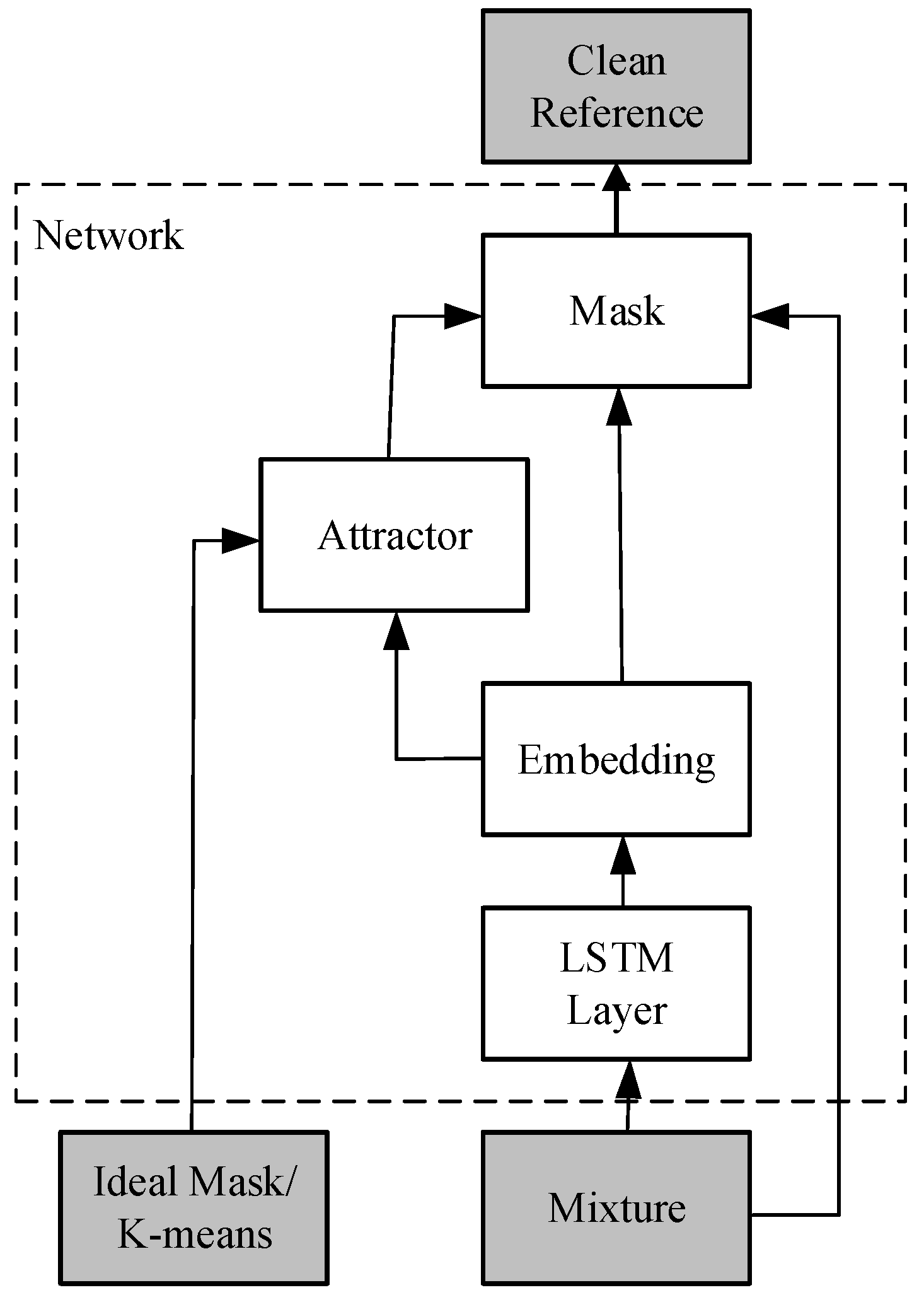
Networks are designed to mimic the biological neural system. In this subsection, we will introduce a neural network model based on the time frequency domain, called the Deep Attractor Network (DANet) [19] as an example. The inspiration for the DANet model comes from a psychological auditory phenomenon in humans known as the perceptual magnet effect [20]. This effect explains how the human brain establishes perceptual attractors for familiar sounds, so that when encountering similar sounds again, the brain can quickly make connections through these attractors, leading to memory and familiarity with the sound.
Figure 1 shows the overall architecture of DANet. Initially, the mixed audio (mixture) undergoes STFT to obtain the time frequency spectrogram. Then, a neural network consisting of four layers of bidirectional long short-term memory (BLSTM) [21] and fully connected layers is used to record the mapping from the time frequency spectrogram to an embedding space. In this embedding space, the mapping of the spectrogram is represented using an embedding matrix , and represents the dimensionality of the embedding space.

Figure 1.
DANet Architecture.
Inspired by the perceptual magnetic effect in humans, attractors can be constructed in the embedding space to serve as reference points for finding speakers with similar characteristics. The construction of attractor A is illustrated in Equation (4).
where represents the number of source speakers, represents the frequency dimension, and represents the time dimension. Y is the source relationship function, which takes a value of 1 when source c has the maximum energy at time t and frequency f, and 0 otherwise. In the embedding space, parts belonging to the same speaker will be closer to their corresponding attractor, while non-corresponding attractors will be relatively farther away. Exploiting this characteristic, the mask M can be estimated using Equation (5).
By estimating the masked audio, it is possible to separate the audio signals using the method described in Section 2.1.
2.2.2. Time Domain-Based Model
In the previous subsection, we introduced a type of speech separation model based on the time frequency domain. These methods operate on the energy spectrogram and estimate masks, resulting in the loss of some phase information. Consequently, the reconstructed signal in the time domain may not achieve the best quality. Additionally, performing STFT requires selecting a suitable frame size, as choosing a frame size that is too small can compromise the effectiveness of the model. This also makes it challenging for the model to achieve real-time processing. As a result, some research has explored alternative approaches that directly utilize the time domain signal, leading to the development of time domain-based model architectures.
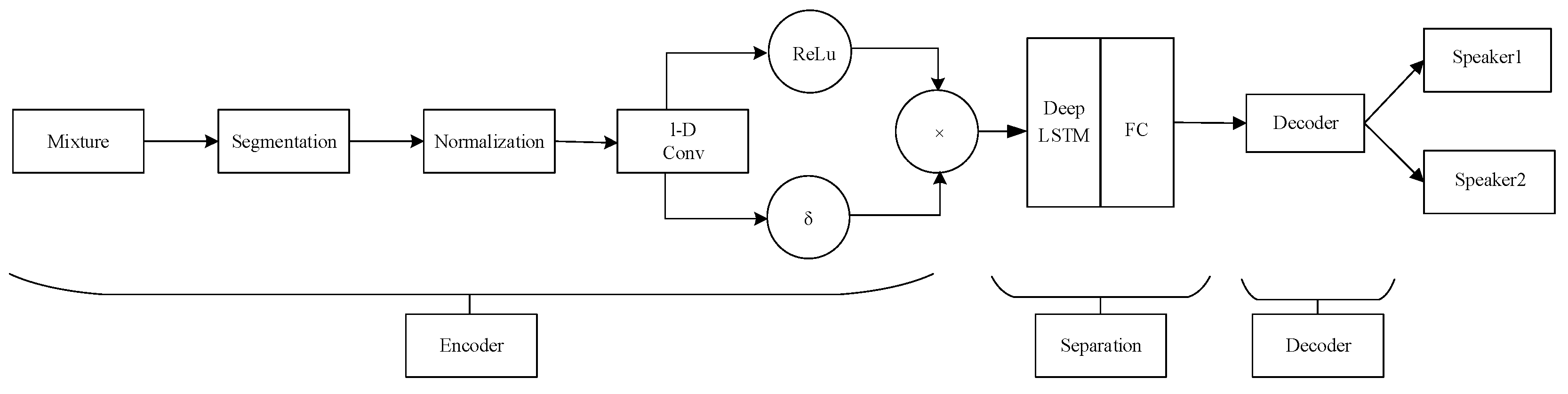
Taking the Time-domain Audio Separation Network (TasNet) [22] as an example, Figure 2 illustrates its architecture. The encoder consists of one-dimensional gated convolutional layers, while the decoder corresponds to one-dimensional deconvolutional layers. In the middle, there is a mask estimation model composed of BLSTM layers and fully connected layers. This architecture allows for the use of smaller time frames and avoids the loss of phase information.
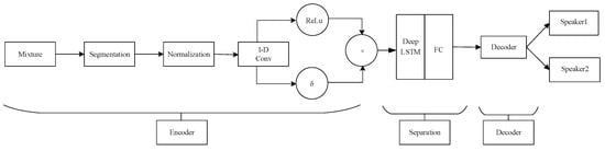
Figure 2.
TasNet Network Architecture.
The encoder, composed of convolutional layers, can be seen as a spatial domain mapping concept that maps the temporal domain signals to a learned latent space. In this space, the neural network model can better discriminate features and estimate masks. The design of the gating mechanism highlights important information. In the middle separation module, several layers of LSTM are used to filter and retain features. Then, through fully connected layers, masks are estimated. The audio signals are mapped to a matrix in the latent space, and a point-wise multiplication is performed to obtain the separated speech signals of each speaker. Finally, the decoder reconstructs the signals back to the temporal domain.
The authors of [22] state that the audio segmentation size of TasNet is 5 ms, which is much smaller than the typical frame size of 32 ms used in STFT. Therefore, TasNet can achieve real-time processing, and the performance of the estimated separated signals in terms of signal-to-noise ratio (SNR) is superior to that of the DANet. Since then, many related studies on speech separation have leaned towards developing methods based on the time domain.
2.2.3. Discussion on the Challenges of above Technology
The previous two subsections provide examples to illustrate speech separation techniques based on different feature domains. However, when it comes to applying these techniques to real-world applications, there are several challenges that need to be overcome.
The first challenge is to separate the individual parts of each speaker from the mixed audio, which requires prior knowledge of the total number of speakers. However, in real-life situations, people can move around and the number of speakers can vary, making it difficult to determine an exact number in advance. This issue further extends to the problem that the trained models cannot generalize well to different numbers of speakers. For example, a model trained on mixed audio from two speakers may not work well for three speakers.
The second challenge involves the permutation problem of the generated masks. For instance, if the produced masks are labeled 1 and 2, it is necessary to know whether these masks correspond to speaker A or B. Incorrect permutations can lead to poor results. Some research has addressed this problem, such as permutation invariant training [23], which exhaustively enumerates all possible combinations to find the permutation with the lowest loss as the correct solution. However, the computational complexity significantly increases as the number of speakers grows. Another approach, recursive speech separation [24], assumes N speakers and separates one speaker from the remaining N − 1 speakers, then repeats the same step for the remaining N − 1 speakers until all speakers are separated. However, this approach can result in decreasing quality for speakers separated later in the process.
2.3. Target Speech Extraction Technique Based on Deep Learning Methods
In Section 2.2.3, discussions were held on some issues encountered in speech separation. As a result, some researchers approached the problem from a different perspective and proposed a method called target speech extraction, which aims to separate the speech of a single target speaker. The advantage of targeting only one speaker is that it avoids certain problems, such as permutation ambiguity, and eliminates the need to know the total number of speakers, as various scenarios can be considered with the target and other interfering sources.
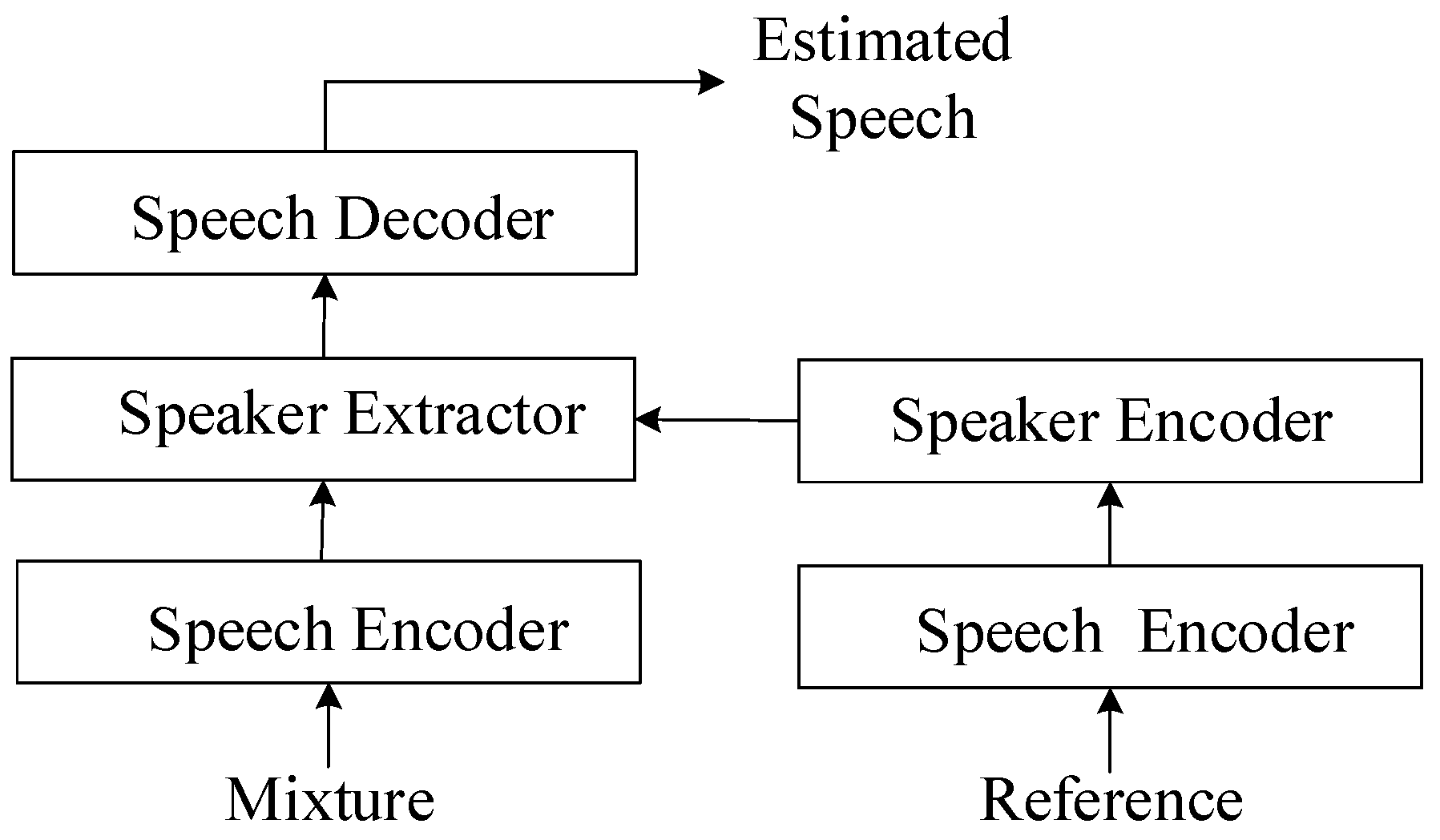
Figure 3 illustrates the basic architecture of the target speech extraction model [25]. The role of the embedder is to map the time domain signal to a feature domain, similar to the STFT or an encoder. To achieve target speech extraction, information about the target is required, typically a short segment of clean speech from the target speaker. Similarly, this speech segment is mapped using the embedder, and then the target information can be summarized using methods like mean pooling to obtain an embedding vector. This embedding vector, along with the input, is fed to the extractor, which utilizes the clues provided by the embedding vector to generate a mask related to the target speaker and ultimately extract the target speech.
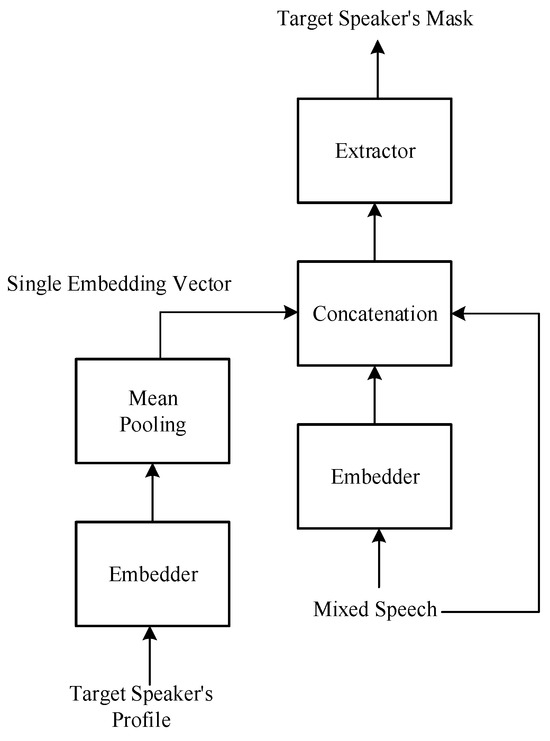
Figure 3.
Basic architecture of the target speech extraction model.
Target speech extraction can be implemented using models based on either the time frequency domain or the time domain, similar to speech separation. In this paper, a time domain model architecture is used, as the problem setting has been modified to avoid some of the challenges encountered in speech separation. Additionally, if information about each speaker is known, separation of all speakers’ audio can be achieved by executing target speech extraction separately for each speaker.
3. Proposed Architecture
3.1. System Architecture
Figure 4 shows the overall system architecture proposed in this paper, which integrates deep learning techniques to achieve target speech extraction. The system architecture can be divided into two stages: the training stage and the testing stage. In the training stage, we will introduce the source and generation methods of the speech dataset, as well as some preprocessing steps before entering the neural network model. Next, we introduce the overall neural network model, which can be divided into four blocks according to their functions: speech encoder, speaker encoder, speaker extractor, and speech decoder. This model structure is based on the SpEx+ [26] baseline model. The difference is that we have additionally added attention-enhancing mechanisms, delay-reducing methods, and used different loss functions. During the training stage, the loss function will be calculated using clean speech, and then the gradient will be updated through backpropagation to minimize the loss function. Additionally, the model’s hyperparameters will be adjusted through validation to facilitate effective learning of the model. In the testing stage, the process is similar to the training stage, but backpropagation and loss function calculation will not be performed. We will use some objective evaluation indicators to measure the quality and efficiency of the system after processing the testing dataset.
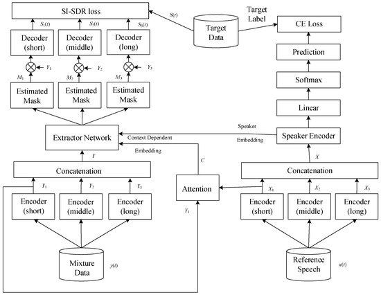
Figure 4.
Proposed system architecture. The system architecture is divided into two stages: the training stage and the testing stage. In the training stage, the source and generation methods of the speech dataset, preprocessing steps, and the overall neural network model are introduced. The neural network model is divided into four blocks: speech encoder, speaker encoder, speaker extractor, and speech decoder. The model structure is based on the SpEx+ baseline model, with additional attention-enhancing mechanisms and delay-reducing methods. In the testing stage, objective evaluation indicators are used to measure the quality and efficiency of the system after processing the testing dataset.
3.2. Training Stage
For the training stage, we first introduce the source and generation of the speech dataset and the preprocessing steps. Then, we introduce various components of the neural network model, which have their own functions and different network structures. Finally, we introduce various types of loss functions, which are used to update the parameters in the model through the calculation of the loss function. Table 1 lists the parameters setting for the training model. After multiple experiments and parameter adjustments, the model is able to converge successfully.

Table 1.
Parameters setting for the training model.
3.2.1. Preprocessing of the Speech Dataset
In this study, the LibriSpeech database [27] was used as the dataset, which contains speech data from audiobooks recorded by LibriVox [27]. The recordings were segmented into clips of 5 to 15 s in length, with a sampling rate of 16KHz. The clips were classified and organized according to the speaker, with a total of 5466 speakers, including males and females of different ages.
We randomly selected 95 speakers for training, validation, and testing datasets. The speakers in the three datasets were not duplicated, making our experiments under opening condition. Two different speakers, one as the target and the other as the interfering speaker, were randomly selected from the dataset. One speech clip in each speaker’s folder was randomly selected for synthesis. The strength of the interference was determined using a signal-to-noise ratio (SNR) between 0 and 5 decibels (dB). In addition, another clean speech clip of the target speaker was randomly selected, as the extraction of the target speech requires a clean speech signal. Both speakers in the synthesized speech clips were used as targets during the dataset composition, doubling the dataset size and balancing the model’s learning.
Finally, the training, validation, and testing datasets contained 37,828, 7188, and 3648 clips, respectively. All audio signals were downsampled to 8 kHz to reduce computational complexity.
3.2.2. Speech Encoder
The speech encoder is the first block in the overall neural network model that receives the audio input, as shown in Figure 5. As there are two segments of audio input, namely the mixture and the reference, there are corresponding encoders for each. The speech encoder is key, initially processing the mixed audio into an abstract form. In parallel, a reference input, a distinct and singular speech signal, is processed using a similar speech encoder. This encoder shares weights with the first, ensuring uniformity in the features it extracts, thus maintaining a balanced audio mapping. The speaker encoder then examines the reference signal to identify unique speaker traits, essential for the following separation phase. These distinctive traits are channeled into the speaker extractor, which employs them to isolate the target speaker’s voice from the mixed audio. The process concludes with the speech decoder, which reconstitutes the estimated speech output, converting the abstract features back into the distinct, isolated audio signal of the target speaker. This complex procedure is fine-tuned through a shared-weight strategy among the encoders during training, fostering consistency and boosting the system’s proficiency in singling out and extracting the desired speech from a noisy backdrop.
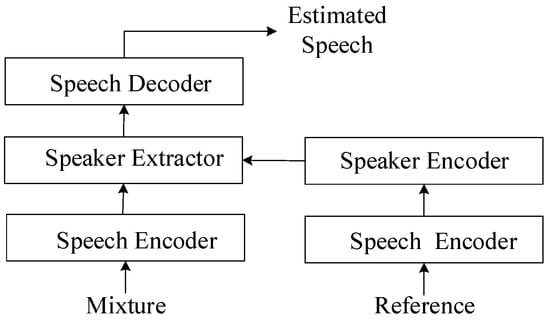
Figure 5.
The role of speech encoder. In the core of this system, the speech encoder plays a crucial role. It acts as the primary entry point, taking in the mixed audio and converting it into a conceptual representation. Simultaneously, a reference input, consisting of a clear, isolated speech signal, undergoes processing using another speech encoder. This second encoder uses the same weights as the first, ensuring that the features it extracts are consistent and aligned. The speaker encoder identifies unique characteristics from the reference, aiding the speaker extractor in isolating the target speaker’s voice. Finally, the speech decoder reconstructs this voice into clear, separated audio, with a weight-sharing strategy across encoders enhancing the system’s effectiveness in noisy environments.
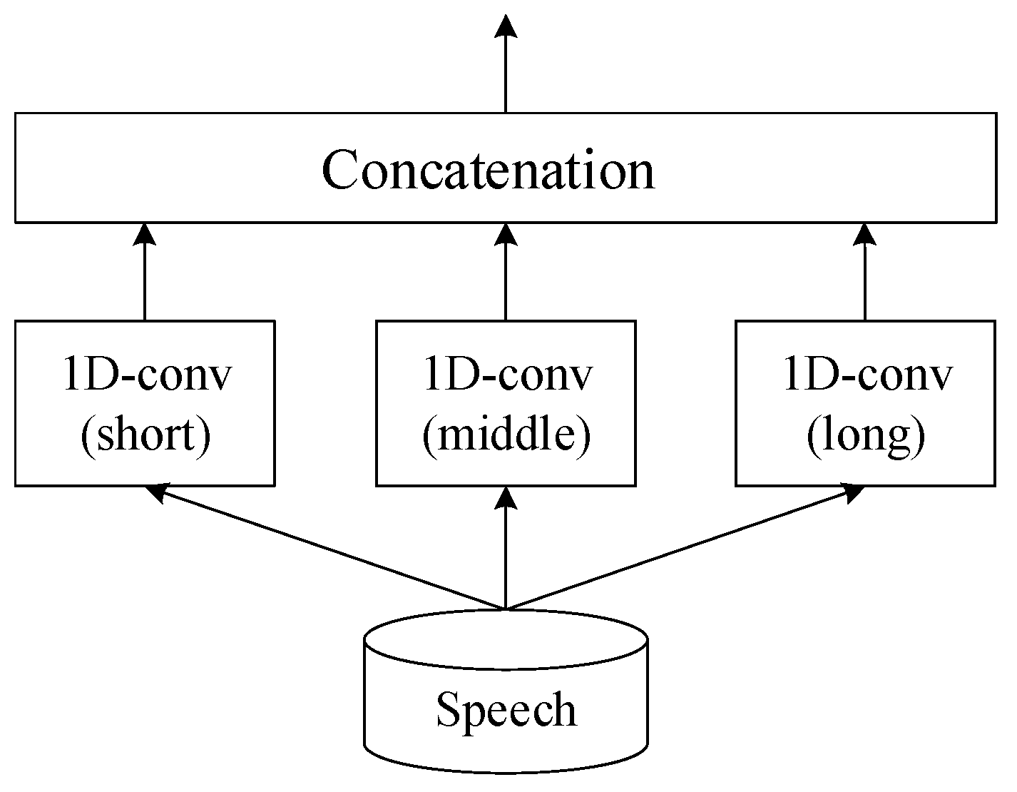
Since speech signals contain a wealth of information, the speech encoder is designed to encode the audio at multiple time scales in order to extract more information. Figure 6 shows the architecture of the speech encoder, which consists of three parallel one-dimensional convolutional layers with different kernel lengths, ranging from short to long, denoted as L1, L2, and L3, respectively. The layer with the shortest kernel, L1, is finely tuned to pick up the minutest aspects of speech, like the tiny tremors in a voice or the rapid pace of speech sounds. This layer is essential for detecting the rapid, transient features in speech. The medium kernel, L2, serves as a bridge, capturing the fundamental elements of spoken language, such as the distinct sounds of vowels and consonants that combine to form words. The longest kernel, L3, captures the broad, sweeping features of speech, such as the rhythm and pitch, which convey the overarching narrative and emotions of the speaker. After processing, the individual feature maps from each layer are combined. This fusion produces a detailed representation of the speech, enabling the encoder to handle complex speech processing by capturing everything from the finest details to the most extensive speech patterns. The different kernel lengths can be considered a type of frame size. The kernel length setting is shown in Table 2.
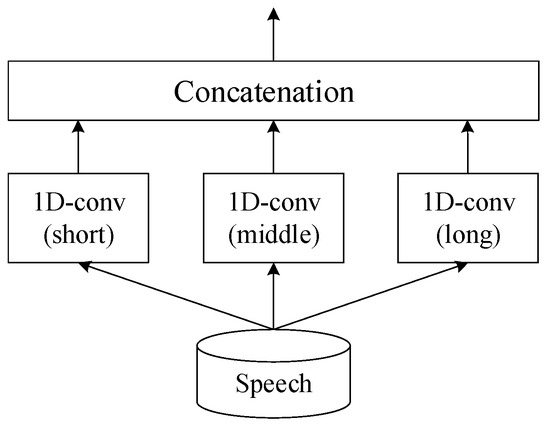
Figure 6.
Architecture of speech encoder outlines an advanced speech encoder framework that precisely extracts features from speech by employing three specialized convolutional layers, each with a unique kernel size. These sizes correspond to different temporal scales: short, medium, and long, allowing the encoder to capture a wide range of speech characteristics.
Table 2.
Kernel length setting for speech encoder.
After the audio is encoded using the three parallel encoders, the results are concatenated, and the stride of the convolutional kernel is set to L1/2 to ensure that the resulting dimensions are consistent. In addition, a stride smaller than the kernel size ensures that important features are not easily lost by providing an opportunity for features to be repeatedly scanned. The audio that needs to be encoded is the mixture audio y(t) and the target reference audio x(t). The encoding process can be represented by Equations (6) and (7), where e(∙) is the encoding function, e(∙), Y and X are the feature matrices concatenated from the mixture and reference audio encodings, θ is the convolutional layer parameter, and N is the dimension size.
3.2.3. Speaker Encoder
The goal of the speaker encoder is to generate appropriate target-embedding vectors to assist the extractor in mask estimation. These embedding vectors can be seen as critical clues with target speaker information, and they can be divided into speaker-embedding vectors and context-dependent embedding vectors.
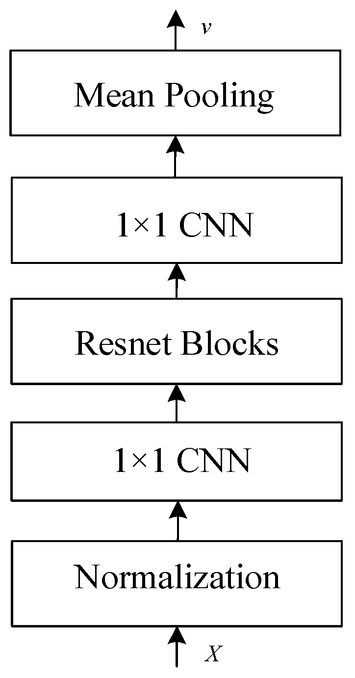
First, we will explain the generation of speaker-embedding vectors. Figure 7 shows the encoder architecture to generate speaker-embedding vectors. The target feature matrix X, which is generated by the audio encoder, is used as input. Layer normalization (LN) [28] is performed first. The operation normalizes all feature dimensions of each individual sample. Then, a 1 × 1 convolutional layer (1 × 1 CNN) is applied, which is a convolutional layer with a kernel size of 1. Its function is to adjust the dimensionality, which can reduce or increase dimensions and allow information to flow between channels. After passing through the 1 × 1 convolutional layer, a residual network (ResNet) [29] is used as the main architecture of the encoder. In this paper, three ResNet blocks are used, and the internal structure of the block is shown in Figure 8. These blocks are designed to help the network learn an identity function, which ensures that the higher layers of the network can perform at least as well as the lower layers, and thus, can avoid the problem of vanishing gradients in deep networks. After the ResNet blocks, another 1 × 1 CNN layer is used to further refine the features extracted via the network. The use of 1 × 1 convolutions helps in reducing the dimensionality and adding non-linearity to the model without affecting the receptive field of the convolutional layers. Finally, mean pooling calculates the mean of the elements in the window of the feature map. Embedding vector (v) captures the characteristics of the speaker’s voice.
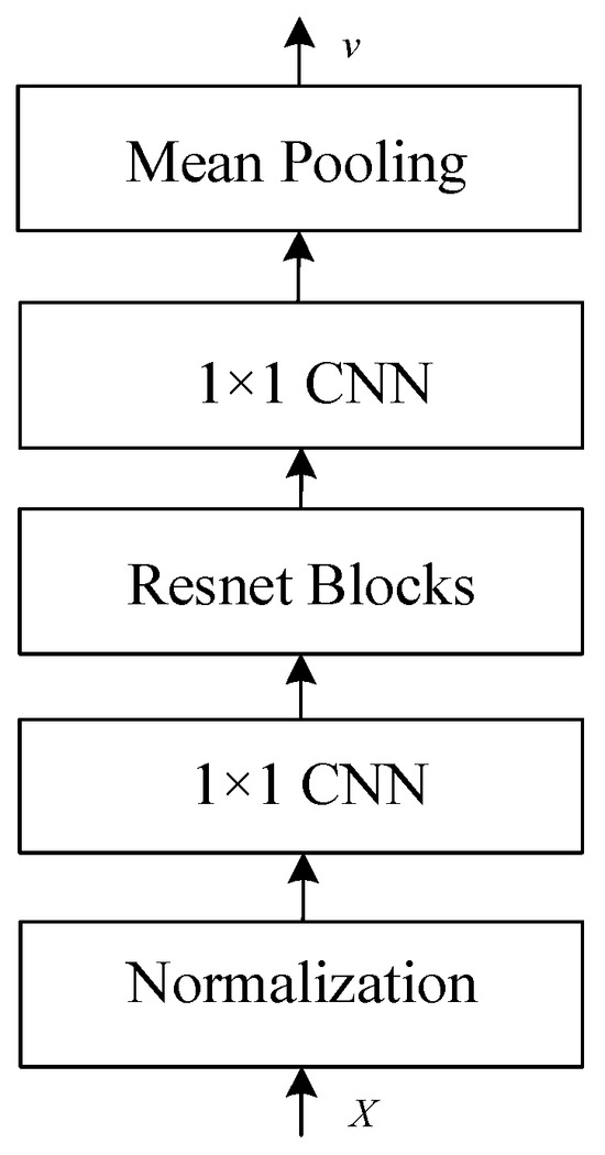
Figure 7.
Architecture of speaker encoder to generate speaker-embedding vectors.
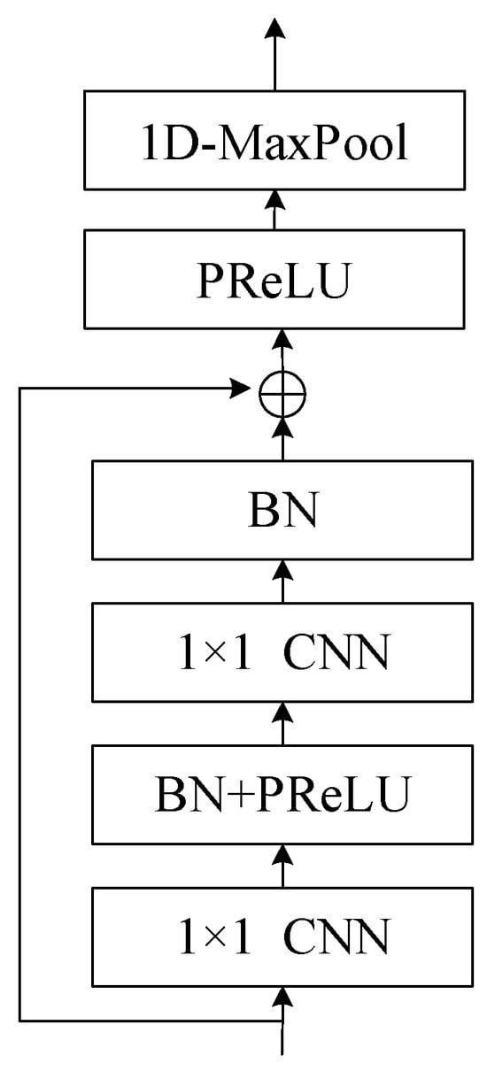
Figure 8.
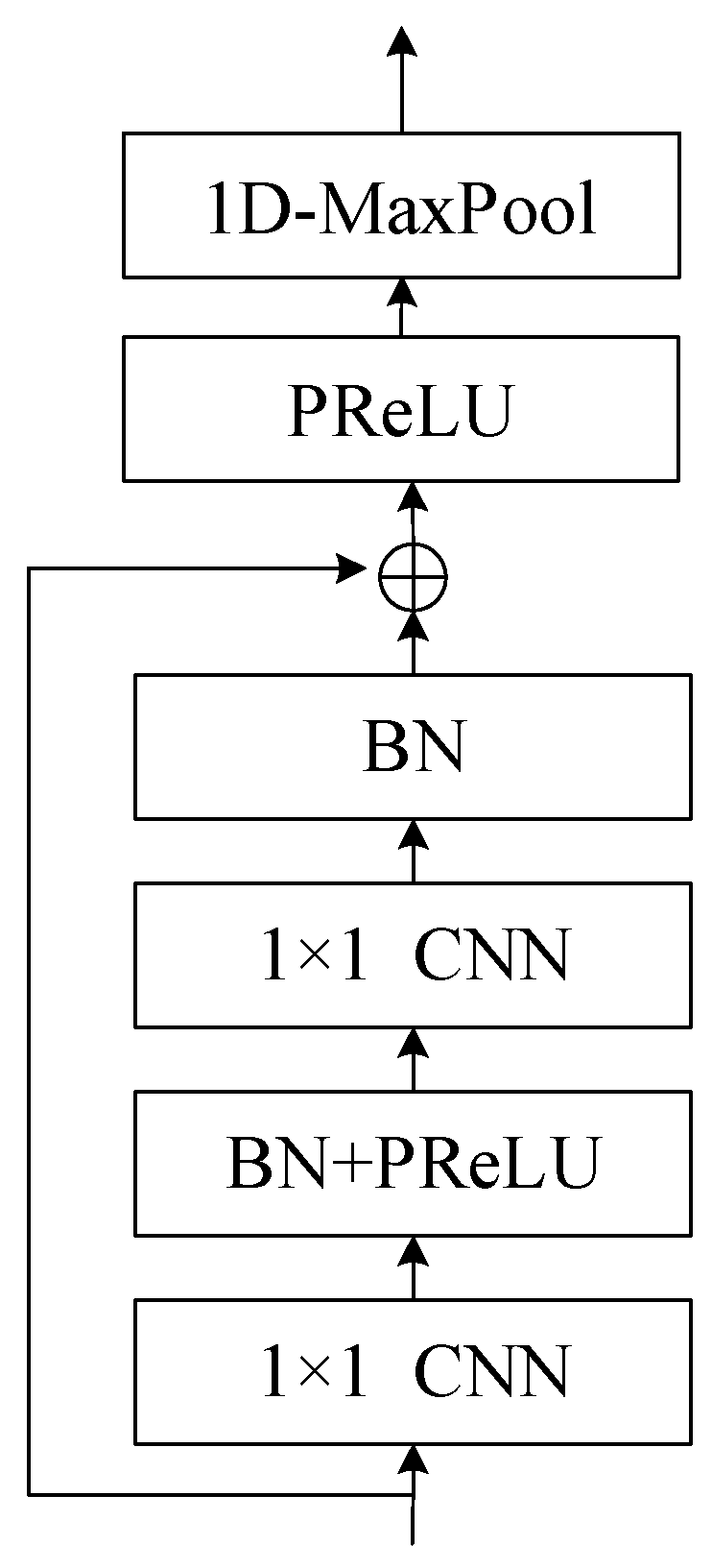
Structure of ResNet block. The ResNet block employs a residual function to capture the difference between learned features and input, ensuring that important information is preserved and preventing degradation in deep networks. The block incorporates 1x1 convolution layers, batch normalization, and PReLU to enhance learning and convergence, while the skip connection adds the input to the learned residual to obtain features. Additionally, a maximum pooling layer is used to remove silent parts of the audio, contributing to the overall effectiveness of the target speech extraction process.
The concept of the residual network is to use skip connections to prevent degradation in deep networks. We use H(x) to represent the features learned by a general neural network, where x is the input. The residual function R(x) can be defined as the difference between H(x) and x, as shown in Equation (8). In other words, the features can be treated as the sum of the residual and the input, as shown in Equation (9).
Thus, if the learning in a layer has no effect, i.e., the residual is zero, the input will be passed to the next layer, preventing degradation. As shown in the structure in Figure 8, two 1 × 1 convolution layers are used to learn the residual, with batch normalization and PReLU interleaved to avoid gradient vanishing and aid convergence. The skip connection adds the input to the learned residual to obtain features, which are then limited in value range using PReLU. At the end of the block, a maximum pooling layer with convolution kernel size of 1 × 3 is used to remove silent parts of the audio. After passing through the ResNet, the dimensions of features are adjusted to be consistent with that of the target speaker-embedding vector using a 1 × 1 convolution layer, and mean pooling is applied along the time dimension to convert the feature matrix into an embedding vector v.
Next, we will introduce the context-dependent embedding vector [25]. Since the speaker-embedding vector is a single one-dimensional vector, its information-carrying capacity is limited. In addition, its vector operations are irrelevant to the model’s input, meaning that the same vector is used regardless of variations in the mixed audio. Therefore, using only this as the target, the embedding vector cannot achieve the best results. In this paper, a method of attention enhancement is proposed to increase the information-carrying capacity of the target embedding vector, which involves adding context-dependent embedding vectors to supplement it. Equations (10)–(12) list the operations of context-dependent embedding vectors.
The target feature matrix and mixed speech feature matrix represent the encoded target reference information and the mixed audio, respectively, where n = 1, 2, 3 corresponds to short, medium, and long encoders, respectively, and are the sizes of the time dimension for the target and mixed features, respectively, and K is the vector dimension. Firstly, an inner product is performed between the two feature matrices based on the feature dimension, resulting in the output at the corresponding time point . Then, the weight vector is computed based on using Equation (11). Finally, the weight vector is multiplied by the corresponding vector in , based on the time point t, and summed to obtain the context-dependent embedding vector at the corresponding time point t.
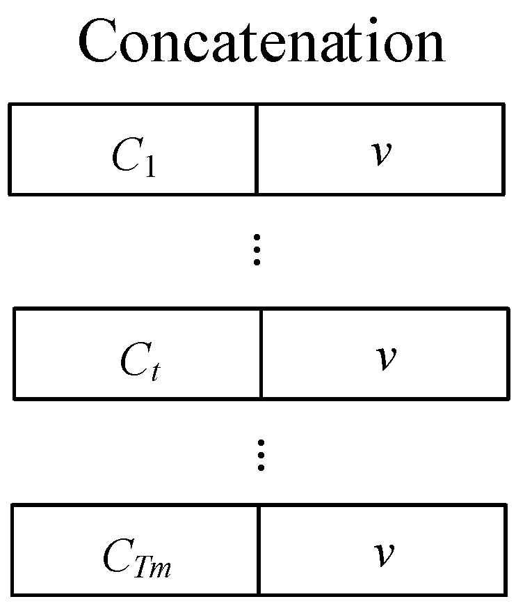
The overall operation can be viewed as considering which part of the reference information to enhance and which part to suppress based on the input mixed speech. That is, using the available information to strengthen the embedding vector. Additionally, the context-dependent embedding vector changes over time and carries richer and varying information, which is expected to help improve performance. We concatenate the speaker-embedding vector v and context-dependent embedding vector based on time to form the target embedding vector, as shown in Figure 9.

Figure 9.
The process of concatenating the speaker-embedding vector and the context-dependent embedding vector to form the target-embedding vector. This step is a crucial part of the target speech extraction process, as it combines speaker-specific features with context-dependent information to create a comprehensive representation of the target speech, ultimately contributing to the effectiveness of the system.
3.2.4. Speaker Extractor
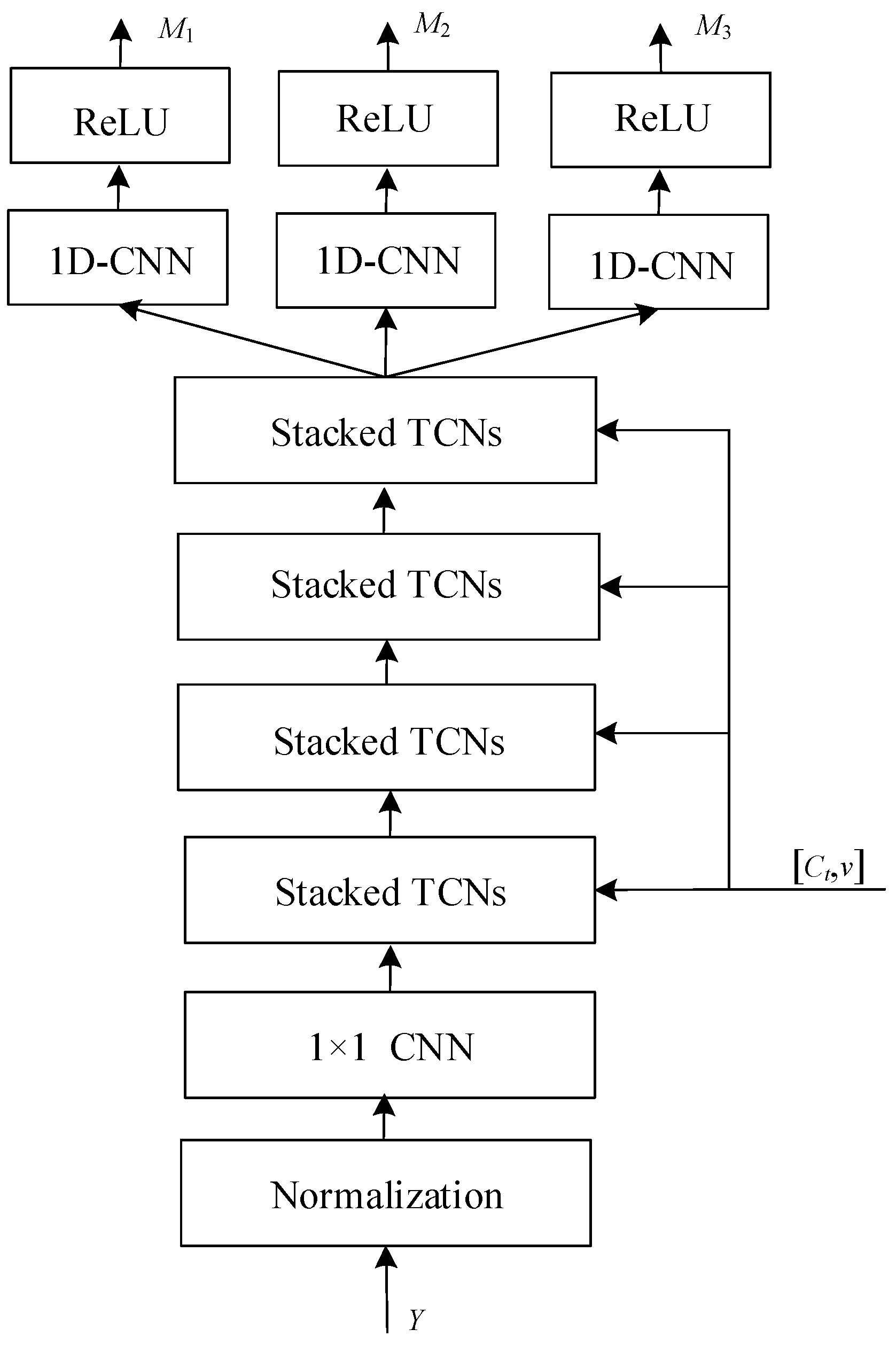
The purpose of the speaker extractor is to use the target embedding vector to estimate the target mask. Figure 10 shows its architecture, which starts with layer normalization and dimension adjustment using a 1 × 1 convolution layer. The input signal y is first normalized to ensure consistency in the range and distribution of input data values, which is crucial for the effective training of neural networks. After normalization, the data is passed through a 1-dimensional convolutional neural network (1D-CNN) layer, which applies a series of filters to extract time-invariant features from the signal. The “1 × 1” refers to the kernel size, meaning that the convolution is applied to each point individually along the time axis. The main body is composed of a temporal convolutional network (TCN) architecture proposed by Conv-TasNet [30], including four stacked TCNs. The stacked TCNs receive the target embedding vector as an additional input to filter the target features. Each TCN block is followed by another 1D-CNN layer, which serves to refine and transform the features further. Each stacked TCN is composed of eight TCN blocks. The rectified linear unit (ReLU) activation function is applied after each 1D-CNN layer. ReLU introduces non-linearity to the model, allowing it to learn more complex functions. Finally, the network outputs multiple embeddings (M1, M2, M3), which are speaker-specific features at various levels of abstraction, corresponding to three encoder lengths.

Figure 10.
Architecture of speaker extractor. This figure presents a multi-stage neural network architecture designed for extracting speaker-specific features from an audio input. The process starts with normalization to standardize input data. It is followed by a sequence of 1D-CNN layers, which apply convolutional filters to extract time domain features. These features are then processed through stacked temporal convolutional networks (TCNs), which are adept at capturing long-range temporal dependencies. Post each TCN block, a 1D-CNN layer refines the features further. ReLU activation functions introduce non-linearity, essential for modeling complex patterns. The architecture concludes with multiple output embeddings M1, M2, M3, representing different levels of feature abstraction, which can be utilized for identifying or verifying speakers.
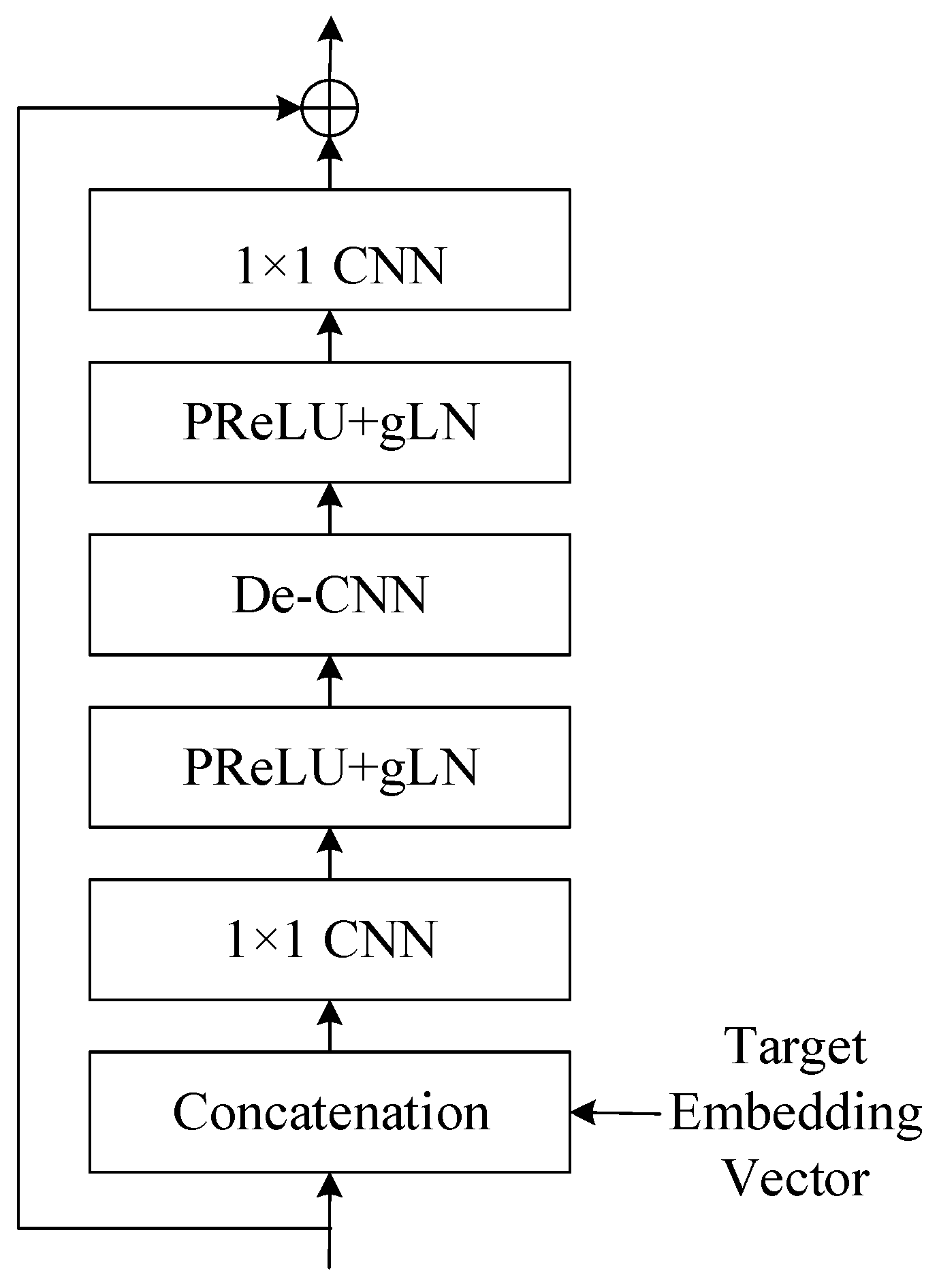
Figure 11 shows the structure of TCN blocks. Only in the first block is the original input concatenated with the target embedding vector as a new input, and this is not done for the other blocks. The process starts with a concatenation step, where an external embedding vector is combined with the block’s input data. This embedding vector typically carries additional information that conditions the layer normalization process. The concatenated output is then passed through a 1-dimensional convolutional neural network (1D-CNN) with a kernel size of 1 × 1. This layer applies a set of filters to learn local patterns within the data. Following the 1 × 1 CNN, the parametric rectified linear unit (PReLU) activation function introduces non-linearity, allowing the model to learn more complex patterns. The activation is followed by a gated layer normalization (gLN), which normalizes the data based on the learned parameters and conditions from the embedding vector, stabilizing the learning process. Next, a depthwise convolutional layer (De-CNN) processes the data. Unlike standard convolutions, depthwise convolutions apply a single filter per input channel, which can efficiently learn spatial hierarchies. The output of the De-CNN goes through another non-linear activation with PReLU followed by gated layer normalization, further refining the features. Another 1 × 1 CNN layer is applied, which can change the dimensionality of the data if necessary and aid in feature transformation. Finally, the processed data is outputted through a residual connection, indicated by the circle with a plus sign. This means that the original input before the block is added to the output, which helps in mitigating the vanishing gradient problem and allows the network to learn an identity function.
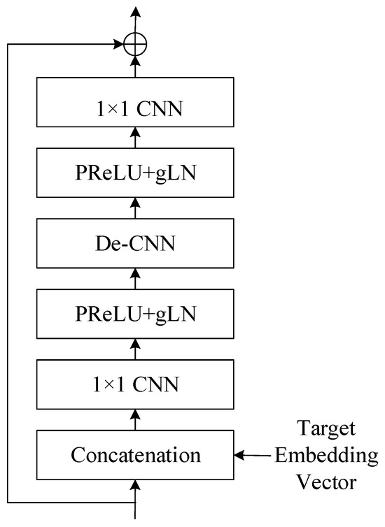
Figure 11.
This figure displays structure of TCN block (cLN ) within a neural network, employing conditional layer normalization for context-specific processing. An embedding vector conditions the input, which then passes through alternating layers of 1 × 1 CNNs and PReLU+gLN for feature extraction and normalization. The structure concludes with a residual connection to ensure smooth training and information flow.
Global layer normalization (gLN) is used in the process, which can be represented by Equations (13)–(15).
where F represents the features of the samples, N is the dimension size of the features, T is the size of the time dimension, λ and τ are parameters obtained through training, and ε is a very small value to prevent division by zero. Equations (13)–(15) compute the mean and variance of each sample dimension before normalization.
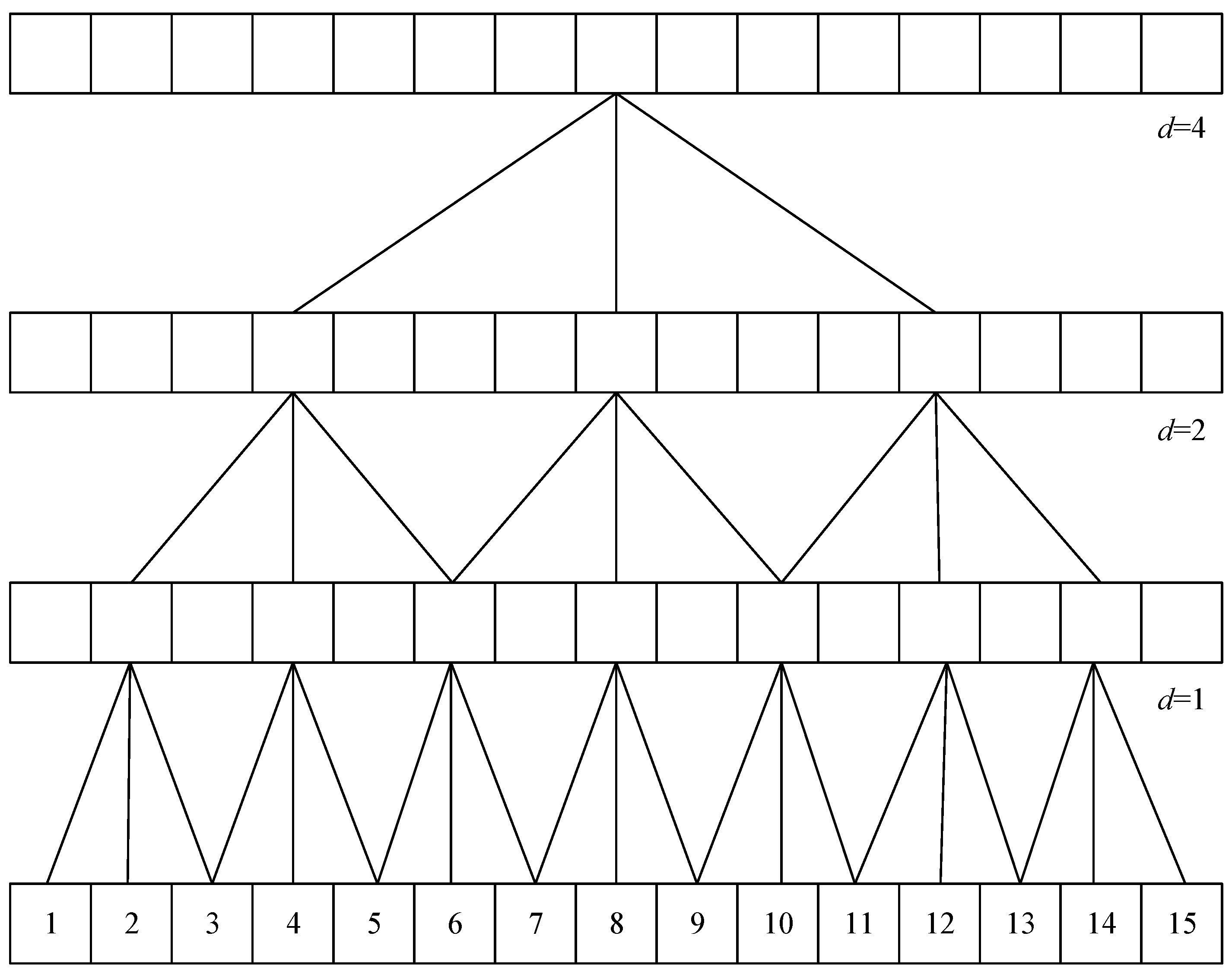
The dilated convolutional layers (De-CNN) [31] is also employed in the model. The special feature of the dilated convolutional layer is that it allows for interval subsampling of the input, meaning that the spacing of each point in the convolutional kernel can be adjusted to create sparse variations. The spacing size is controlled by the dilation factor d, which is 1 in normal convolutional layers. In the TCN module, the dilation factor is set to for the eight blocks, where b = 0, 1, 2, …, 7, as shown in Figure 12. The deeper the block, the larger the spacing, which means that the receptive field expands and the computation cost is reduced. By using different receptive field sizes, the convolutional neural network can learn different combinations of feature variations and understand the degree of temporal changes, enabling the network to have the ability to interpret temporal significance.
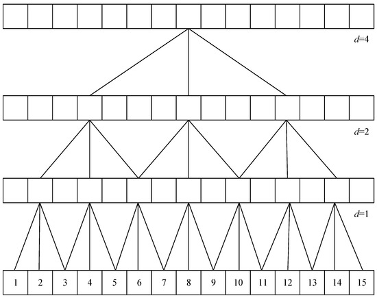
Figure 12.
Dilated convolutional layer with increasing dilation rates at different levels. It allows the network to aggregate information over larger receptive fields without losing resolution. At the bottom level (d = 1), the convolution has no dilation, operating on adjacent data points. As we move up, the dilation rate increases, with d = 2 skipping one data point and d = 4 skipping three, enabling the layer to cover more extensive data spans effectively.
The baseline model used in this study employs non-causal convolutions in its dilated convolutional layers, which cover feature information from future time steps, requiring some delay in computation to obtain future information. This paper proposes a latency reduction method that can be flexibly adjusted. The extractor includes four TCN modules, with eight TCN blocks in each module, making it a deep neural network model with many layers. Using non-causal convolution, the delay for each layer accumulates to a considerable amount of time. To speed up computation, we can replace dilated convolutions with causal convolutions, which only cover present and past time steps, and padding is used to facilitate the operation. The 1 × 1 convolution layer remains unchanged because its kernel size is 1, so it does not use past or future information. In addition, we also change the global layer normalization to cumulative layer normalization (cLN) [32] to accommodate causal convolutions. The computation of cLN is represented by Equations (16)–(18).
where represents the feature F from the beginning of time to time point k. The rest of the calculation is the same as normal layer normalization, i.e., only normalizing the information from the past to the present.
When the temporal convolutional network is composed of causal convolutions, the latency can be reduced, but since it only utilizes past information, its performance may be slightly worse than non-causal convolutions. By adjusting the ratio of the TCN blocks with non-causal and causal convolutions in the temporal convolutional network of the extractor, we can obtain the trade-off between latency and performance, and obtain the most suitable state based on the application requirements.
3.2.5. Audio Decoder
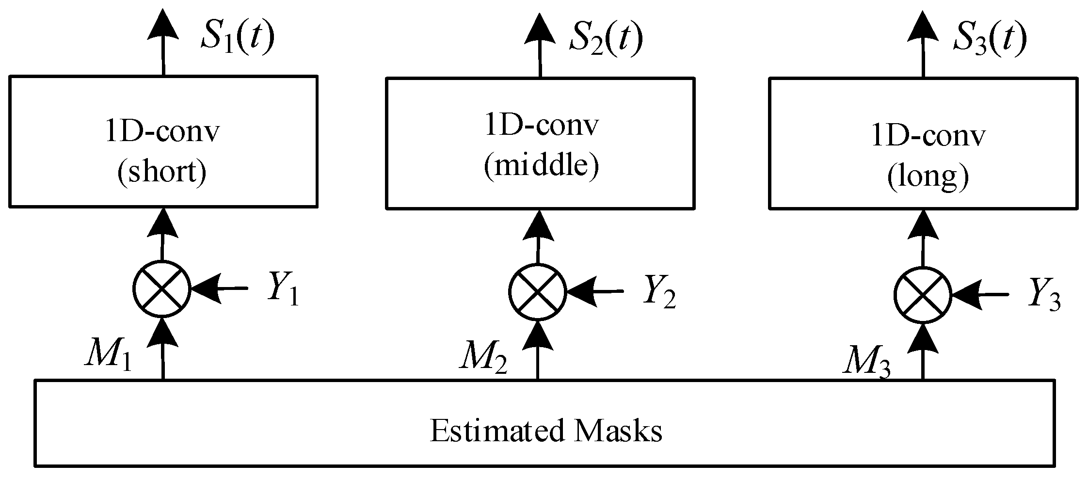
In the speaker extractor, three masks corresponding to different lengths of audio encoders are generated as the final output, as shown in Figure 13. Then, we use these masks and three parallel 1D convolutional layers corresponding to the respective audio encoders as the decoder to separate the target speech from the mixed speech. The operation of the decoder, de(∙), can be expressed as Equation (19).
where ⨂ denotes element-wise multiplication between matrices, represents the mask for the corresponding encoder–decoder of different lengths, and is the estimated target speech obtained via the corresponding encoder–decoder operation. The final estimated speech is then used to calculate the loss function to assist in updating the parameters of the neural network model.
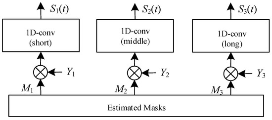
Figure 13.
Architecture of audio decoder (Y3 is missing). It is responsible for differentiating and isolating a target speaker’s voice from a mixture of speech. Within this component, three masks are generated, each associated with convolutional layers of varying lengths—short, middle, and long. These masks play an essential role in the speech separation process.
3.2.6. Loss Function
In the speaker extractor, three masks corresponding to different lengths of audio encoders are generated as the final output, as shown in Figure 13. Then, we use these masks and three parallel 1D convolutional layers corresponding to the respective audio encoders as the decoder to separate the target speech from the mixed speech. The operation of the decoder, de(∙), can be expressed as Equation (19).
In the training process of the neural network model, the calculation of the loss function is an important step. The result of the loss function is used for backpropagation to update the model’s parameter weights. In this subsection, we introduce the loss function used in the proposed neural network model. The neural network model can be viewed as a multi-task learning model, where there are two tasks. One is to generate effective speaker-embedding vectors, and the other is to extract high-quality target speech. Therefore, suitable loss functions are set for these two tasks, and then combined to form the overall loss function of the model.
Firstly, we introduce the loss function used to evaluate speaker-embedding vectors. We adopt the cross-entropy loss (CE loss), represented by Equation (20).
where is the total number of speakers, represents the correct label for the speaker, σ(⋅) is the softmax function, and W is the weight matrix. The entire calculation is a speaker recognition task, where the softmax function is used to predict the probability of each speaker, and the sum of all predicted probabilities is equal to 1. Finally, the cross-entropy loss function is calculated to measure whether the embedding vector v can correctly identify the target speaker.
Next, we introduce the loss function used to evaluate the quality of the generated speech. We use the multi-scale reconstruction loss function, which can be represented by Equation (21):
In the model, there are three encoders with different time scales, resulting in three estimated target speech segments. We calculate the loss function of each segment with respect to the reference ground truth and obtain , where is a certain time domain speech loss function. The weighted sum of the three loss functions, with weights α and β, is calculated as the overall loss.
In the baseline model, the scale invariant signal-to-distortion ratio (SI-SDR) is used as the loss function for . The SI-SDR is calculated as shown in Equation (22).
where denotes the reconstructed signal, represents the absolute-value norm, and the scaling factor . The difference between SI-SDR and the commonly used signal-to-noise ratio (SNR) is that SI-SDR uses the scaling factor to stretch or shrink the reference signal, so that the error vector between the reconstructed signal, and the reference signal is orthogonal to the reference signal vector. Therefore, the ratio obtained via the SI-SDR calculation is more objective as it is based on the same reference standard.
However, the scaling factor used relies on the reconstructed signal, so its errors need to be taken into account. This paper proposes using the scale dependent signal-to-distortion ratio (SD-SDR) [4] as the loss function. Considering that the scaling factor also has errors, two types of errors need to be calculated: the error of the scaling factor and the error of the reconstructed signal, as expressed by Equation (23).
where the scaling factor error is represented as , and the reconstruction error is represented as . Substituting the calculated results into Equation (22), we obtain the SD-SDR Equation (24).
Finally, we combine the multi-scale reconstruction loss function with the cross-entropy loss function to form the overall loss function, as shown in Equation (25), where γ is a proportion parameter. Table 3 lists the parameter setting for the loss function.
Table 3.
Parameter setting for the loss function.
3.3. Testing Stage
During the testing stage, we used a testing dataset to evaluate the performance of the trained neural network model. For each testing data point, the input to the model is a mixture of speech and a reference audio signal of the target, and the model produces an estimated target speech through forward propagation without computing the loss function. For evaluation, we selected the best SD-SDR among the results generated via the three decoders as the representative for calculation. We evaluated the results based on two commonly used methods in speech processing research: scale-invariant signal-to-distortion ratio (SI-SDR) and perceptual evaluation of speech quality (PESQ).
PESQ is a method for evaluating the perceived quality of speech. It quantifies the difference in speech quality between the estimated speech and the clean speech, and the results are scored using the mean opinion score (MOS) evaluation method in narrowband conditions, with scores ranging from −0.5 to 4.5, with higher values indicating better speech quality.
4. Experimental Results and Discussion
4.1. Experimental Environment
We used Pytorch as the framework to construct the neural network model and Matlab for pre-processing operations on the speech dataset. During the training stage, we utilized a GPU GeForce GTX 2080 to accelerate the training and convergence of the neural network, in order to reduce the time spent. Table 4 shows the configuration of the hardware and software environment for the experiments.
Table 4.
Hardware and software environments for the experiments.
4.2. Experimental Results Comparison and Discussion
In this section, we will present comparisons of attention mechanisms using different sources, comparisons between the proposed system and other methods, comparisons of the effectiveness of the latency reduction method, and discuss the results separately.
4.2.1. Comparisons of Attention Mechanisms Using Different Sources
In Section 3.2.3, we introduced the proposed attention-enhanced mechanism, which can use feature matrices generated by audio encoders of different lengths to compute context-dependent embedding vectors. Since encoders of different lengths map signals to different latent feature spaces, we conducted experiments to compare the effects of different sources of embedding vectors on the overall performance. The different sources are feature matrices corresponding to three encoders. Table 5 shows the comparison results.
Table 5.
Comparison results of attention mechanisms using different sources.
The three corresponding feature matrices were generated via short, medium, and long encoders, denoted as L1, L2, and L3, respectively. The evaluation was presented in terms of SI-SDR and PESQ. According to the results, the use of feature matrices from the short-length encoder produced the best results, achieving the highest values in both SI-SDR and PESQ. This is because the use of very short convolution kernel sizes in the encoder can scan the signal in detail for each small time frame, obtaining the features it contains. In particular, the window size of 2.5 ms is much smaller than the commonly used window size of 32 ms for STFT calculations, which makes it easier to fully perceive the fine-grained features. After being filtered by the neural network, important information can be better preserved, which contributes to the improvement of system performance.
4.2.2. Comparisons between the Proposed System and Other Methods
To evaluate the performance of the proposed system, we compared it with other studies on target speech extraction. The compared models include the baseline model SpEx+ [26], its predecessor model SpEx [33], and the model SBF-MTSAL-Concat [34]. The baseline model and its predecessor, as well as the proposed system, are all based on the time domain method, while the SBF-MTSAL-Concat model is based on the time frequency domain method. There are differences among the three methods, including the generation of embedding vectors using different methods. SBF-MTSAL-Concat and SpEx use bidirectional long short-term memory networks (BLSTM) to generate embedding vectors, while SpEx+ is similar to the proposed method in using residual neural networks (ResNet) to generate embedding vectors. In addition, the proposed method incorporates an attention mechanism to enhance the embedding vectors. Regarding the neural network models for estimating the masks, the time frequency domain method uses a recurrent neural network architecture, which is BLSTM, while the time domain method uses a convolutional neural network architecture, which is a TCN. Furthermore, in terms of calculating the loss function, the time frequency domain method tends to use the spectrogram to compute, while the time domain method tends to use the reconstructed audio to compute.
Table 6 presents the comparisons between the proposed system and other methods. In the proposed method, we use the conclusion of Section 4.2.1, where we generate context embedding vectors using the feature matrix obtained via the L1 length encoder, and compare the results of using SI-SDR or SD-SDR to calculate the reconstruction error loss in the loss function. It can be observed that using SD-SDR leads to the best performance. This can be explained by the derivation process and Equation (24) of SD-SDR discussed in Section 3.2.6. Since SD-SDR takes into account the scaling factor error, it can provide a more robust performance when comparing the correct signal vector with the error vector. Moreover, the denominator of the simplified Equation (24) is , which is the absolute value norm of the difference between the correct signal and the reconstructed signal. By minimizing the loss function, the neural network model can be intuitively encouraged to produce reconstructed signals that are close to the correct signal. The results also show that methods based on the time domain generally outperform those based on the time frequency domain, which is why more recent research tends to focus on time domain methods or a combination of both.
Table 6.
Comparisons between the proposed system and other methods.
4.2.3. Comparisons of the Effectiveness of the Latency Reduction Method
In this subsection, we will compare and discuss the proposed latency reduction method, without using GPU for computation. Two models are used for comparison, one is the baseline model SpEx+, and the other is the proposed system using the best settings from the previous experiments, which is the combination of Attention (L1) and SD-SDR. Table 7 shows the comparison results, where the symbol * indicates that all TCN blocks in the model use causal dilated convolution and cumulative layer normalization. Processing time refers to the average time in seconds taken by the model to process one second of audio from input to output. From the results, we can see that the proposed latency reduction method can reduce the processing time by about 22%, but the speech quality may degrade. Also, the processing time does not solely come from TCN blocks, but mostly from audio and speaker encoders. Furthermore, the table only compares models using either all causal or all non-causal operations, but the proposed method can adjust the proportion of the two types of TCN blocks according to need, and the reduction time and the degradation in quality should be within the range of the values listed in Table 7, which represents the upper and lower bounds of the performance.
Table 7.
Comparisons of the effectiveness of the latency reduction method.
4.2.4. Comparisons the Effectiveness for Different Numbers of Speakers
In this subsection, we will discuss the differences and effects of different numbers of speakers in mixed signals. Table 8 shows the performance differences of our proposed method for different numbers of total speakers. “2-speakers (3-spk-test)” means that the model is trained with mixed audio containing two speakers, but tested with mixed audio containing three speakers; “2-speakers” means that the model is trained and tested with mixed audio containing two speakers; “3-speakers” means that the model is trained and tested with mixed audio containing three speakers. From the results, we can see that if the number of speakers in the test mixed audio is different from that in the training data, the performance will not be as good. Therefore, to extract speech from situations with different numbers of speakers, a model trained with the corresponding number of speakers is needed. Additionally, as the number of speakers in the mixed audio increases, the performance of extracting the target speaker’s speech will also deteriorate. In summary, in order to have a wider and more convenient application in practical situations, developing a standardized model that can handle different numbers of speakers can also be a key focus of future development.
Table 8.
Comparisons the effectiveness for different numbers of speakers.
4.3. Discussion
The results presented in the tables offer insightful revelations about the performance of various attention mechanisms and processing methods in target speaker extraction. A critical aspect of these findings is their implications for human perception, particularly in how listeners discern and evaluate the extracted speech. Firstly, the comparison of different attention mechanisms (Table 5) underscores a significant variation in SI-SDR values, with Attention (L2) achieving the highest score. This suggests its superior capability in reducing signal distortion, which is crucial for maintaining the integrity of the original speech.
In the broader system comparisons (Table 6), the proposed method with Attention (L1) demonstrates an enhancement in both SI-SDR and PESQ over the baseline and other methods. This improvement is pivotal from a human perception standpoint, as it suggests a more natural and clearer listening experience. The slight variations observed with different ρ formulas also point to the nuanced ways in which algorithmic changes can impact perceived audio quality.
The effectiveness of the latency reduction method (Table 7) brings to light the trade-off between processing speed and audio quality. From a user experience perspective, while faster processing is desirable, it should not come at the cost of noticeably poorer audio quality. The reduced SI-SDR and PESQ scores in the faster processing settings might lead to a less satisfactory listening experience, indicating the challenge of balancing efficiency and quality in real-time applications.
Finally, the performance variation with different numbers of speakers (Table 8) is particularly relevant to human perception in complex auditory environments. The decline in performance metrics with an increased number of speakers mirrors the challenges faced by human listeners in multi-talker situations. The system’s reduced effectiveness in these scenarios may lead to a less accurate representation of the target speaker, potentially impacting the listener’s ability to focus on the desired speech amidst background noise and other speakers. Overall, the results showed that the proposed attention mechanism using feature matrices from the short-length encoder produced the best results, achieving the highest values in both SI-SDR and PESQ. This suggests that the use of very short convolution kernel sizes in the encoder can capture detailed signal features, leading to improved system performance.
5. Conclusions
This paper proposes a neural network model based on temporal convolutional networks and attention-enhanced mechanisms for target speech extraction. In some previous methods, speech separation was used to address the cocktail party problem. However, this approach encountered two main challenges: the need to know the total number of speakers in advance and the permutation problem of masks. Subsequent research efforts have focused on target speech extraction to overcome these challenges. While frequency domain methods are limited by phase information loss and frame size restrictions, time domain methods have also been explored. For target speech extraction, a single normalized embedding vector cannot provide sufficient information to the model.
Our proposed method builds upon previous research and experience, adopting a time domain approach. To address the issue of single normalized embeddings, we introduce an attention-enhanced mechanism that provides context-based and time-varying embeddings, thereby enhancing the information carried by the model. Experimental results confirm that this mechanism improves speech quality. We also propose a latency reduction method to mitigate the accumulated delay caused by deep temporal neural networks. This method demonstrates reduced computation time in the experimental results without sacrificing speech quality. Furthermore, the method is not fixed and allows for a trade-off between time and quality depending on the application. In terms of loss function calculation, we discuss the drawbacks of SI-SDR and propose the use of SD-SDR, which yields better results in the experimental evaluations.
Author Contributions
Conceptualization, J.-C.W., P.T.L. and P.-C.C.; Methodology, Y.-T.L.; writing—original draft preparation, Y.-T.L.; writing—review and editing, J.-H.W., T.-C.T., T.P., Z.-Y.W. and Y.-H.L.; supervision, P.-C.C. All authors have read and agreed to the published version of the manuscript.
Funding
This study was partially supported by the National Science and Technology Council of Taiwan under Grant 110-2221-E-008-076-MY3.
Institutional Review Board Statement
Not applicable.
Informed Consent Statement
Not applicable.
Data Availability Statement
The data presented in this study are openly available at http://www.openslr.org/12/ (accessed on 15 May 2014) [19].
Conflicts of Interest
The authors declare no conflicts of interest.
References
- Cherry, E.C. Some experiments on the recognition of speech, with one and with two ears. J. Acoust. Soc. Am. 1953, 25, 975–979. [Google Scholar] [CrossRef]
- Pedersen, M.S.; Wang, D.; Larsen, J.; Kjems, U. Two-microphone separation of speech mixtures. IEEE Trans. Neural Netw. 2008, 19, 475–492. [Google Scholar] [CrossRef] [PubMed]
- Bartelds, M.; San, N.; McDonnell, B.; Jurafsky, D.; Wieling, M. Making More of Little Data: Improving Low-Resource Automatic Speech Recognition Using Data Augmentation. arXiv 2023, arXiv:2305.10951. [Google Scholar]
- Li, J. Recent advances in end-to-end automatic speech recognition. APSIPA Trans. Signal Inf. Process. 2022, 11, e8. [Google Scholar] [CrossRef]
- Feng, S.; Halpern, B.M.; Kudina, O.; Scharenborg, O. Towards inclusive automatic speech recognition. Comput. Speech Lang. 2024, 84, 101567. [Google Scholar] [CrossRef]
- Zhang, Y.; Ma, Y.; Liu, Y. Convolution-bidirectional temporal convolutional network for protein secondary structure prediction. IEEE Access 2022, 10, 117469–117476. [Google Scholar] [CrossRef]
- Roux, J.L.; Wisdom, S.; Erdogan, H.; Hershey, J.R. SDR—Half-baked or well done. In Proceedings of the 2019 IEEE International Conference on Acoustics, Speech and Signal Processing (ICASSP), Brighton, UK, 12–17 May 2019; pp. 626–630. [Google Scholar]
- Luo, Y.; Chen, Z.; Yoshioka, T. Dual-path rnn: Efficient long sequence modeling for time-domain single-channel speech separation. In Proceedings of the ICASSP 2020–2020 IEEE International Conference on Acoustics, Speech and Signal Processing (ICASSP), Barcelona, Spain, 4–8 May 2020; pp. 46–50. [Google Scholar]
- Hu, X.; Li, K.; Zhang, W.; Luo, Y.; Lemercier, J.M.; Gerkmann, T. Speech separation using an asynchronous fully recurrent convolutional neural network. Adv. Neural Inf. Process. Syst. 2021, 34, 22509–22522. [Google Scholar]
- Wang, Z.Q.; Wang, D. Combining spectral and spatial features for deep learning based blind speaker separation. IEEE/ACM Trans. Audio Speech Lang. Process. 2018, 27, 457–468. [Google Scholar] [CrossRef]
- Wang, Z.-Q.; Roux, J.L.; Wang, D.; Hershey, J.R. End-to-end speech separation with unfolded iterative phase reconstruction. arXiv 2018, arXiv:1804.10204. [Google Scholar]
- Liu, W.; Liao, Q.; Qiao, F.; Xia, W.; Wang, C.; Lombardi, F. Approximate designs for fast Fourier transform (FFT) with application to speech recognition. IEEE Trans. Circuits Syst. I Regul. Pap. 2019, 66, 4727–4739. [Google Scholar] [CrossRef]
- Yan, B.C.; Wu, M.C.; Chen, B. Exploring feature enhancement in the modulation spectrum domain via ideal ratio mask for robust speech recognition. In Proceedings of the 2020 Asia-Pacific Signal and Information Processing Association Annual Summit and Conference (APSIPA ASC), Auckland, New Zealand, 7–10 December 2020; pp. 759–763. [Google Scholar]
- Ha, M.T.; Liang, K.W.; Lee, Y.S.; Lee, C.T.; Li, Y.H.; Wang, J.C. Speech separation using augmented-discrimination learning on squash-norm embedding vector and node encoder. IEEE Access 2022, 10, 102048–102063. [Google Scholar]
- Luo, Y.; Mesgarani, N. Tasnet: Time-domain audio separation network for real-time, single-channel speech separation. In Proceedings of the 2018 IEEE International Conference on Acoustics, Speech and Signal Processing (ICASSP), Calgary, AB, Canada, 15–20 April 2018; pp. 696–700. [Google Scholar]
- Tan, H.M.; Vu, D.Q.; Wang, J.C. SeliNet: A lightweight model for single channel speech separation. In Proceedings of the 2023 IEEE International Conference on Acoustics, Speech and Signal Processing (ICASSP), Rhodes Island, Greece, 4–10 June 2023; pp. 1–5. [Google Scholar]
- Wang, Y.; Narayanan, A.; Wang, D. On training targets for supervised speech separation. IEEE/ACM Trans. Audio Speech Lang. Process. 2014, 22, 1849–1858. [Google Scholar] [CrossRef] [PubMed]
- Lee, Y.S.; Kuo, Y.; Chen, S.H.; Wang, J.C. Discriminative training of complex-valued deep recurrent neural network for singing voice separation. In Proceedings of the 2017 ACM Multimedia Conference (ACM MM), Mountain View, CA, USA, 23–27 October 2017; pp. 1327–1335. [Google Scholar]
- Chen, Z.; Luo, Y.; Mesgarani, N. Deep attractor network for single-microphone speaker separation. In Proceedings of the 2017 IEEE International Conference on Acoustics, Speech and Signal Processing (ICASSP), New Orleans, LA, USA, 5–9 March 2017; pp. 246–250. [Google Scholar]
- Kuhl, P.K. Human adults and human infants show a perceptual magnet effect. Percept. Psychophys. 1991, 50, 93–107. [Google Scholar] [CrossRef] [PubMed]
- Alamsyah, R.D.; Suyanto, S. Speech gender classification using bidirectional long short term memory. In Proceedings of the 2020 3rd International Seminar on Research of Information Technology and Intelligent Systems (ISRITI), Yogyakarta, Indonesia, 10–11 December 2020; pp. 646–649. [Google Scholar]
- Luo, Y.; Mesgarani, N. Real-time single-channel dereverberation and separation with time-domain audio separation network. In Proceedings of the Interspeech 2018, Hyderabad, India, 2–6 September 2018; pp. 342–346. [Google Scholar]
- Yu, D.; Kolbak, M.; Tan, Z.H.; Jensen, J. Permutation invariant training of deep models for speaker-independent multi-talker speech separation. In Proceedings of the 2017 IEEE International Conference on Acoustics, Speech and Signal Processing (ICASSP), New Orleans, LA, USA, 5–9 March 2017; pp. 241–245. [Google Scholar]
- Takahashi, N.; Parthasaarathy, S.; Goswami, N.; Mitsufuji, Y. Recursive speech separation for unknown number of speakers. In Proceedings of the Interspeech 2019, Graz, Austria, 15–19 September 2019; pp. 1348–1352. [Google Scholar]
- Xiao, X.; Chen, Z.; Yoshioka, T.; Erdogan, H.; Liu, C.; Dimitriadis, D.; Droppo, J.; Gong, Y. Single-channel speech extraction using speaker inventory and attention network. In Proceedings of the 2019 IEEE International Conference on Acoustics, Speech and Signal Processing (ICASSP), Brighton, UK, 12–17 May 2019; pp. 86–90. [Google Scholar]
- Ge, M.; Xu, C.; Wang, L.; Chng, E.S.; Dang, J.; Li, H. SpEx+: A complete time domain speaker extraction network. In Proceedings of the Interspeech 2020, Shanghai, China, 25–29 October 2020; pp. 1406–1410. [Google Scholar]
- Panayotov, V.; Chen, G.; Povey, D.; Khudanpur, S. Librispeech: An ASR corpus based on public domain audio books. In Proceedings of the 2015 IEEE International Conference on Acoustics, Speech and Signal Processing (ICASSP), South Brisbane, QLD, Australia, 19–24 April 2015; pp. 5206–5210. [Google Scholar]
- Ba, J.L.; Kiros, J.R.; Hinton, G.E. Layer normalization. arXiv 2016, arXiv:1607.06450. [Google Scholar]
- He, K.; Zhang, X.; Ren, S.; Sun, J. Deep residual learning for image recognition. In Proceedings of the 2016 IEEE Conference on Computer Vision and Pattern Recognition (CVPR), Las Vegas, NV, USA, 27–30 June 2016; pp. 770–778. [Google Scholar]
- Luo, Y.; Mesgarani, N. Conv-tasnet: Surpassing ideal time–frequency magnitude masking for speech separation. IEEE/ACM Trans. Audio Speech Lang. Process. 2019, 27, 1256–1266. [Google Scholar] [CrossRef] [PubMed]
- Juyal, P.; Kundaliya, A. Multilabel image classification using the CNN and DC-CNN model on Pascal VOC 2012 dataset. In Proceedings of the 2023 International Conference on Sustainable Computing and Smart Systems (ICSCSS), Coimbatore, India, 14–16 June 2023; pp. 452–459. [Google Scholar]
- Guo, J.I.; Tsai, C.C.; Tseng, C.K. Pvalite CLN: Lightweight object detection with classification and localization network. In Proceedings of the 2019 32nd IEEE International System-on-Chip Conference (SOCC), Singapore, 3–6 September 2019; pp. 118–121. [Google Scholar]
- Xu, C.; Rao, W.; Chng, E.S.; Li, H. SpEx: Multi-scale time domain speaker extraction network. IEEE/ACM Trans. Audio Speech Lang. Process. 2020, 28, 1370–1384. [Google Scholar] [CrossRef]
- Xu, C.; Rao, W.; Chng, E.S.; Li, H. Optimization of speaker extraction neural network with magnitude and temporal spectrum approximation loss. In Proceedings of the 2019 IEEE International Conference on Acoustics, Speech and Signal Processing (ICASSP), Brighton, UK, 12–17 May 2019; pp. 6990–6994. [Google Scholar]


Disclaimer/Publisher’s Note: The statements, opinions and data contained in all publications are solely those of the individual author(s) and contributor(s) and not of MDPI and/or the editor(s). MDPI and/or the editor(s) disclaim responsibility for any injury to people or property resulting from any ideas, methods, instructions or products referred to in the content. |
© 2024 by the authors. Licensee MDPI, Basel, Switzerland. This article is an open access article distributed under the terms and conditions of the Creative Commons Attribution (CC BY) license (https://creativecommons.org/licenses/by/4.0/).