1. Introduction
Antenna arrays play a crucial role in various industries of modern information technology, including radar, communications, remote sensing, etc. [
1,
2,
3,
4,
5,
6]. Beamforming, as a fundamental technique in array signal processing, is widely employed to enhance target signal and suppress interference by creating deep nulls in undesired directions. Improving the interference suppression capability of antenna arrays is a critical requirement for radar and communication systems.
Over the past few decades, numerous beamforming techniques have been investigated [
7,
8,
9,
10,
11,
12,
13]. Conventional beamforming techniques require adjusting the amplitude and phase of the receive filter, resulting in higher hardware costs at the receiver. Therefore, previous works have explored phase-only beamforming techniques for phased array radar [
10,
11,
12,
13], which utilize neural networks [
10], numerical optimization [
11], and other methods [
12,
13] to obtain phase-only weights. However, these techniques may be limited by computational complexity. In order to reduce computational complexity and improve practicality, a phase-only array response adjustment via the geometric approach was proposed [
14]. Unfortunately, this method [
14] can only rapidly adjust the response at a single point and cannot simultaneously form deep nulls for multiple points. Moreover, it is worth noting that these techniques [
7,
8,
9,
10,
11,
12,
13,
14] primarily aim to create deep nulls in desired directions, but they are limited in their ability to create deep nulls at specific locations due to the angle-dependent beam pattern of phased array radar systems. From a practical point of view, it is possible to encounter interference signals that have similar angles as the target of interest [
15,
16]. As a result, there is a demand to investigate beamforming techniques that can effectively form deep nulls at specific locations.
Recently, the frequency diverse array (FDA) radar has gained significant attention from academia due to its degrees of freedom (DOFs) in the range domain [
17,
18,
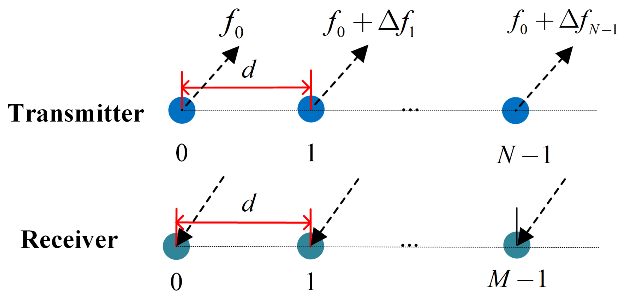
19]. In contrast to the capability of forming nulls in a specific direction in the beam pattern of phased array radar, by introducing frequency offsets between the elements of the transmitter, FDA allows for the control of nulls in both range and angle dimensions, thus effectively suppressing interference signals from specific directions and ranges. However, the beam pattern of the FDA radar exhibits time-varying characteristics, necessitating the integration of Multiple-Input Multiple-Output (MIMO) technology at the receiver end to achieve an equivalent time-invariant beam pattern [
20,
21,
22], thereby fully leveraging the advantages of the two-dimensional (2D) range-angle beam pattern of the FDA radar.
Based on this capability, numerous beamforming techniques [
23,
24,
25,
26,
27] have been proposed. For instance, Lan et al. [
26] proposed two iterative algorithms with multi-response control based on the oblique projection (MRCOP) method, namely the concurrent MRCOP (C-MRCOP) and the successive MRCOP (S-MRCOP). Moreover, two approaches, namely point-by-point successive null broadening control (SNBC) and multi-point concurrent null broadening control (CNBC), were developed for suppressing interference [
27]. These approaches [
27] were designed to broaden nulls at specific positions and effectively mitigate interference signals. Apart from the aforementioned works, there are various other beamforming techniques for the FDA-MIMO radar, such as transmit beam space design [
28], cognitive FDA-MIMO radar beamforming [
29], low probability of intercept of FDA-MIMO radar beamforming [
30], and so on [
31,
32,
33]. It is worth noting that none of the aforementioned methods investigate the phase-only beamforming technique for the FDA-MIMO radar. This implies that the mentioned approaches are not capable of utilizing phase shifters at the receiver to form deep nulls at desired positions. Thus, the implementation of these methods requires a complex and high-cost hardware architecture. For the FDA-MIMO radar, two data-independent phase-only beamforming methods were proposed using the convex optimization technique [
34]. However, these methods still have computational complexities, and cannot find an efficient solution in polynomial time when the number of antennas is large. To the best of our knowledge, there have been limited reports on the fast phase-only beamforming technique for the FDA-MIMO radar.
Motivated by this research gap, we propose a fast phase-only beamforming method via the Kronecker decomposition [
35] for the FDA-MIMO radar. In our work, we utilize the Kronecker decomposition to decompose the desired phase-only weight vectors into phase-only transmit and receive weight vectors, and decompose the target steering vector into transmit and receive steering vectors. The steering vectors and weight vectors of the transmit and receive modes with the Vandermonde structure are then decomposed into Kronecker factors with uni-modulus vectors, respectively. Subsequently, we divide the Kronecker factors into two parts to achieve interference suppression and signal enhancement. Our algorithm can rapidly form a deep null at the desired position with low computational complexities. Numerical experiment results demonstrate the effectiveness and superiority of the proposed method. We briefly summarize the research contributions of our work as follows:
- (1)
We propose a phase-only beamforming design algorithm for the FDA-MIMO radar based on Kronecker decomposition.
- (2)
We offer an analytical solution of the interference suppression factors and signal enhancement factors.
- (3)
The proposed algorithm can form deep nulls at specified locations with very low complexity and reduce the hardware cost of the FDA-MIMO radar system.
The remainder of this paper is organized as follows. In
Section 2, the system model is introduced, and the problem formulation is presented.
Section 3 presents the analytical solution for phase-only weight by designing the interference suppression factors and signal enhancement factors. Numerical simulations are employed in
Section 4 to validate the effectiveness of the proposed method. Finally, concluding remarks are provided in
Section 5.
Notations: Throughout this paper, notations , and are used to represent the conjugate, transpose and conjugate transposes, respectively. denotes the modulus of complex number w. ⊗ represents the Kronecker product. is the phase of . represents the Euclidean norm of a vector. outputs the remainder after dividing by . Π denotes the cumulative product operation. refers to the orthogonal space of . represents the identity matrix, and indicates the sets of the complex matrix.
3. The Phase-Only Beamforming Based on Kronecker Decomposition
In this section, we introduce a fast phase-only beamforming technique via Kronecker decomposition for the FDA-MIMO radar. For simplicity, we hypothesize that the numbers of transmitter and receiver satisfy
and
, where
P and
Q are positive integer (we discuss the general case where the number of the transmitter or receiver is an arbitrary positive integer in
Section 3.4).
3.1. The Proposed Phase-Only Weight Vector Design Model
For the convenience of subsequent calculation, before designing the phase-only weight vector, we define weight vector
to be a feasible solution to Problem (12) with the following form:
where
and
are defined as the transmit and receive weight vectors, respectively. Next, we introduce the following problem (14):
where
and
represent the target transmit and receive steering vectors, respectively.
and
are the
jth interference transmit and receive steering vectors, respectively. Compared to Problem (12), in Problem (14), variable
is replaced with
and
. Moreover, to maximize SINR, we expect the left side of (12c) to be as small as possible and set the left-hand side of Constraint (14c) equal to zero. In the next section, we present an approach based on Kronecker decomposition to design phase-only weight vectors
and
.
3.2. Kronecker Decomposition of Weight Vector and Steering Vector
First of all, we introduce an important lemma on Kronecker decomposition.
Lemma 1 (Kronecker Decomposition [
35]).
Let us consider vector whose elements have uni-modulus and which has a Vandermonde structure according to the following expression:where Φ is fixed. Vector can be decomposed as , where with being positive integers. Each factor with a length of is given by with .
We note that if
, then
in Lemma 1 is now simplified as
. Recalling the transmit and receive steering vectors in (
6) and (
7), we can observe that
and
exhibit a Vandermonde structure, as stated in
Lemma 1. Hence,
and
can be decomposed as (
16) and (
17), respectively.
where
and
denote the transmit and receive Kronecker factors, respectively (
and
), which are defined as
where
.
According to Problem (14), the design of
and
must satisfy (14b) for target echo enhancement and (14c) for interference suppression. To meet these requirements and simplify the algorithm, we assume that weight vectors
and
have a Vandermonde structure. Then,
and
are decomposed as
where
and
denote the
pth and
qth Kronecker factors of the transmit and receive weight vectors, respectively. Building upon Equations (
20) and (
21), the design of
and
is converted into the design of
and
. We introduce the design method of the Kronecker factors and synthesize the phase-only weight vector in the next subsection.
3.3. Design the Phase-Only Weight Vector
In the previous subsection, based on the Kronecker decomposition, the steering vector and the weight vector are decomposed into multiple Kronecker factors. In accordance with Equations (
16), (
17), (
20) and (
21), we can express
as follows:
Based on the mathematical properties of the Kronecker product, it is known that for any matrices
,
, and
, they satisfy
. Then,
is equivalent to
where Equation (25) is derived from the fact that
and
are complex numbers.
By observing Equation (25), we can find out, for the jth interference, that an arbitrary needs to be designed such that satisfies onstraint (14c) for interference suppression, where (, and . Similarly, to satisfy target echo enhancement Constraint (14b), the rest of needs to be designed to maximize . For convenience, we designate the Kronecker factors that satisfy Constraint (14b) as Signal Enhancement (SE) factors and denote their set as . Conversely, the remaining Kronecker factors used to fulfill Constraint (14c) are referred to as Interference Suppression (IS) factors, with their set denoted as . It follows that . Additionally, we define , where denotes the set of transmit and receive steering vector factors of the target or interference. We further define as the target set and as the jth interference set.
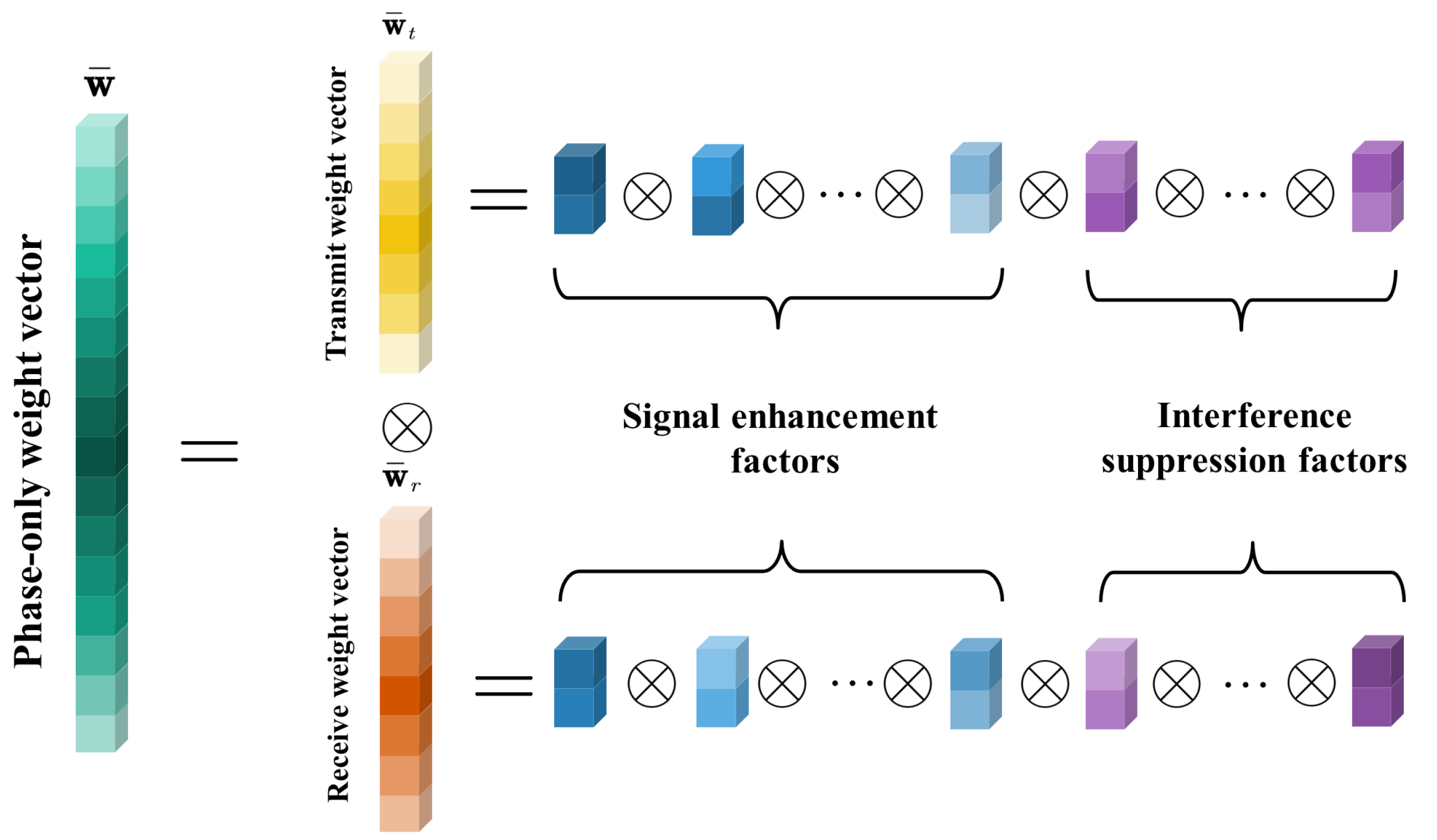
Now, we can design IS and SE factors separately to synthesize phase-only vector
. For the convenience of understanding, we offer a relatively intuitive diagram
Figure 2 where we can clearly see that the phase-only weight is decomposed into multiple Kronecker factors.
3.3.1. The Design of Interference Suppression Factors
As described in Problem (14), for any interference, the expected weight vector should satisfy Constraint (14c). Then, according to Equation (25), Constraint (14c) for
jth interference steering vector
is assumed to be
Using sets
and
, Equation (
26) can be simply expressed as
where
,
.
One can observe from Equation (
27) that for the
jth interference, we only need to choose one of the Kronecker products,
, such that the equation equals zero. Since
is fixed, the selection process of Kronecker product
is equivalent to selecting
or
from the set
. The chosen
is assigned to the corresponding Kronecker product factor in (
27) for each
jth interference equation, and
is called the IS factor. We suppose the superscript of the chosen IS factor for the
jth interference is
; based on Equation (
27), the
th Kronecker product factor should satisfy Equation (
28).
where
. We recall Equations (
20) and (
21); the specific form of
can be defined as
For the
jth equation, if
, substituting (
29) and (
18) into (
28), the unknown phase of the vector
can be expressed as
If
in the
jth equation, substituting (
29) and (
19) into (
28), the unknown phase of the vector
can be expressed as
where
and
denote the transmit and receive spatial frequencies of the
jth interference, respectively.
The phase solutions to (
30) are
and the phase solutions to (
31) are
It is important to note that arbitrarily chosen
satisfies Constraints (14d) or (14e), but not arbitrary
can maximize the value of
in (14b). Once the IS factors are determined, based on (25),
can be written as
where
. In order to design the weight vector and ensure maximizing
in Constraint (14b), we expect (
36) to be as large as possible. Thus, we calculate all the
and choose
with the largest modal value. The selected
is able to obtain the maximum
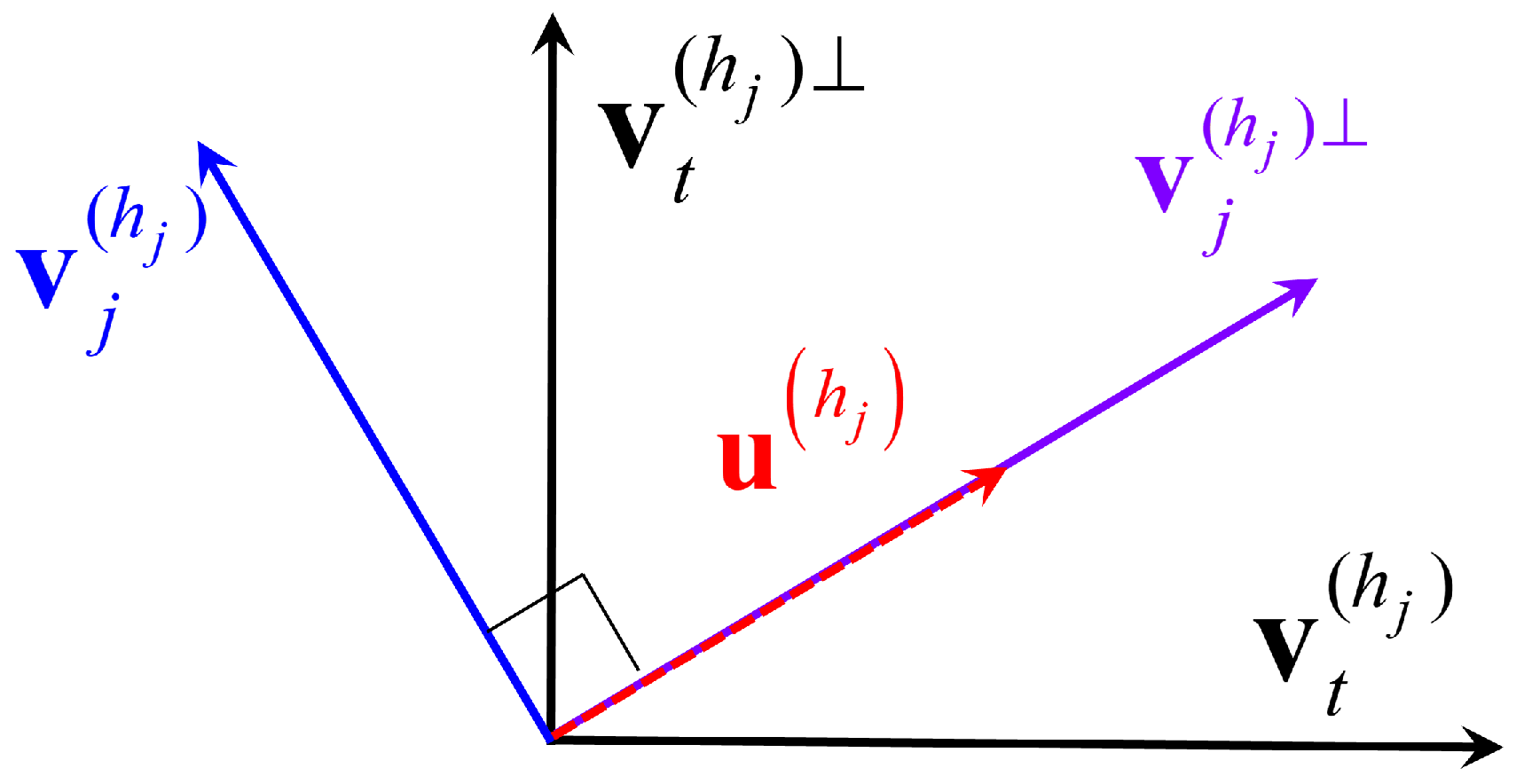
, that is, the target echo gain. For easy understanding of the relation between Kronecker factors and steering vector factors, the geometric perspective is shown in
Figure 3. The calculated
is actually in orthogonal space
of
, and the process of selecting
is essentially to find orthogonal space
with the smallest angle with
.
In summary, the criterion for the determination of the IS factors effectively suppresses the interference signal while ensuring the maximization of the output SINR. The design procedure of IS factors is summarized in Algorithm 1 with specific steps elaborated.
| Algorithm 1 Design of IS factors. |
- Require:
, , and . - Ensure:
All the IS factors . - 1:
Set . - 2:
. - 3:
. - 4:
. - 5:
for each do - 6:
. - 7:
. - 8:
. - 9:
end for - 10:
for each do - 11:
for each do - 12:
. - 13:
if then - 14:
. - 15:
else - 16:
. - 17:
end if - 18:
Calculate . - 19:
end for - 20:
Choose the with largest as the j-th IS factor - 21:
end for
|
3.3.2. The Design of Signal Enhancement Factors
After obtaining the IS factors in , there are still SE factors to be designed. In other words, Kronecker product factors in need to be designed to maximize (enhanced signal power) and meet Constraints (14d) and (14e) (satisfy the phase-only constraint).
By pooling the designed IS factors corresponding to all
J interferences, denoting the superscript of the SE factors as
, Constraint (14b) can be expressed as
where
and
both belong to the set
. Following Definitions (
6) and (
7) and Constraints (14d) and (14e), we can easily observe that the module of the
th Kronecker product factor is not greater than 2. This implies that
Observing Equation (
38), we know that
obtains its maximum value only when
and
are conjugate with each other, i.e.,
. According to Definitions (
18) and (
19), we define
to have the following form:
where
or
is chosen according to the value of
;
and
denote the transmit and receive spatial frequencies of the target, respectively.
Thus, when
, the phase solutions to
are
We note that arbitrarily
satisfies Constraints (14d) or (14e). In summary, the SE factors can be determined, and steps are summarized in Algorithm 2.
| Algorithm 2 Design of SE factors |
- Require:
. - Ensure:
All the SE factors . - 1:
for each do - 2:
if then - 3:
- 4:
else - 5:
if then - 6:
- 7:
end if - 8:
end if - 9:
end for
|
With the two aforementioned algorithms, the SE and IS factors can be determined. The transmit and receive weight vectors can be calculated using the Kronecker product as specified in Equations (
20) and (
21), respectively. The final phase-only weight vector is calculated from Equation (
13). Then, the design procedure of the phase-only weight vector is given in Algorithm 3.
| Algorithm 3 Design of Phase-Only Weight Vectors |
- Require:
and . - Ensure:
The phase-only weight vector . - 1:
Select and design IS factors by performing Algorithm 1 - 2:
Design SE factors by performing Algorithm 2. - 3:
Calculate the transmit weight vector . - 4:
Calculate the receive weight vector . - 5:
Calculate the weight vector .
|
3.4. Discussion
In this subsection, we discuss the performance of the proposed phase-only beamforming algorithm, including the antenna number, IS factors selection, bistatic FDA-MIMO radar, and computation complexity.
3.4.1. Antenna Number
The weight vector is designed for the exceptional case when the number of transmitter and receiver
and
. In fact, for the general case of non-prime number, it can perform the Kronecker decomposition. After the Kronecker decomposition of
and
, they can be decomposed into Kronecker factors of the following form:
The transmit and receive weight vectors can be determined using the procedures described in the previous section.
According to reference [
35], when the number of antennas is a prime number, one simple solution is to utilize antenna selection. This approach addresses the issue of the inability to decompose the steering vector into Kronecker products. For instance, in the case where there are 67 antennas, the optimal subset of 64 antennas can be chosen using a specific selection criterion. These selected 64 antennas can then be employed for phase-only beamforming using Kronecker decomposition. Additionally, it is mentioned in [
35] that standards such as IEEE 802.11n and IEEE 802.11ac [
36] often set the number of antennas to be a power of two. This aligns well with the proposed design, facilitating the application of the proposed approach.
3.4.2. Interference Suppression Factors Selection
In Algorithm 1, we consider the common case where each interference has different transmit and receive frequencies, that is, and . This means that the corresponding and for different interferences are not the same. Therefore, for the jth interference, the obtained can only be used to suppress the jth interference. If there are multiple interferences with a common transmit or receive frequency, it is possible to design an IS factor that can suppress both interferences simultaneously. This means that for different interferences, there is a shared component in (the transmit or receive Kronecker factors), and they have a common such that .
Moreover, it is important to note that the proposed algorithm exhibits a high demand for array DOFs due to the relationship between the number of IS and SE factors and the number of array elements. As the number of interferences increases, there is a degradation in beam performance for a given number of array elements. Furthermore, accurate a priori information is required by the proposed algorithm, indicating its limited robustness.
3.4.3. Bistatic FDA-MIMO Radar
In this subsection, we discuss the application of the proposed algorithm to a bistatic FDA-MIMO radar. According to the steps of the proposed algorithm, the calculation of the phase-only weight vector is related to the transmit and receive spatial frequencies of the interference and the target. For a bistatic FDA-MIMO radar, we let represent the direction of arrival and denote the direction of departure. The transmit and receive spatial frequencies of the bistatic FDA-MIMO radar are denoted as and , respectively. Therefore, when computing IS and SE factors in Algorithms 1 and 2, it is necessary to substitute the transmit and receive spatial frequencies with those of the bistatic FDA-MIMO radar.
3.4.4. Computation Complexity
It is worth highlighting that the proposed phase-only beamforming algorithm has low computational complexities. The computational cost of the algorithm primarily arises from the calculation of the phases of IS and the SE factors, including only the simple additions or multiplication operators. In the Algorithm 1 part, the computational complexity mainly arises from the calculation of phase solution
and the calculation of
. Since
and
with the dimension of
, the computational complexity of
is
. The computational load of calculating the solution of
in (
33) or (
35) is
. So the computational complexity of Algorithm 1 is
. In addition, the complexity of Algorithm 2 is
. Based on the analyses above, the computational complexity of the proposed algorithm is
, where
. In contrast, the convex optimization method in [
34] requires
complex operations, and the SNBC method in [
27] requires
complex operations.
Table 1 summarizes the computational complexity of these algorithms.


