
Common-Mode Voltage Suppression of a Five-Level Converter Based on Multimode Characteristics of Selective Harmonic Elimination PWM


Abstract
:1. Introduction
2. Illustration of Selective Harmonic Elimination Pulse-Width Modulation Technique and Common-Mode Voltage Problem for Five-Level Converter
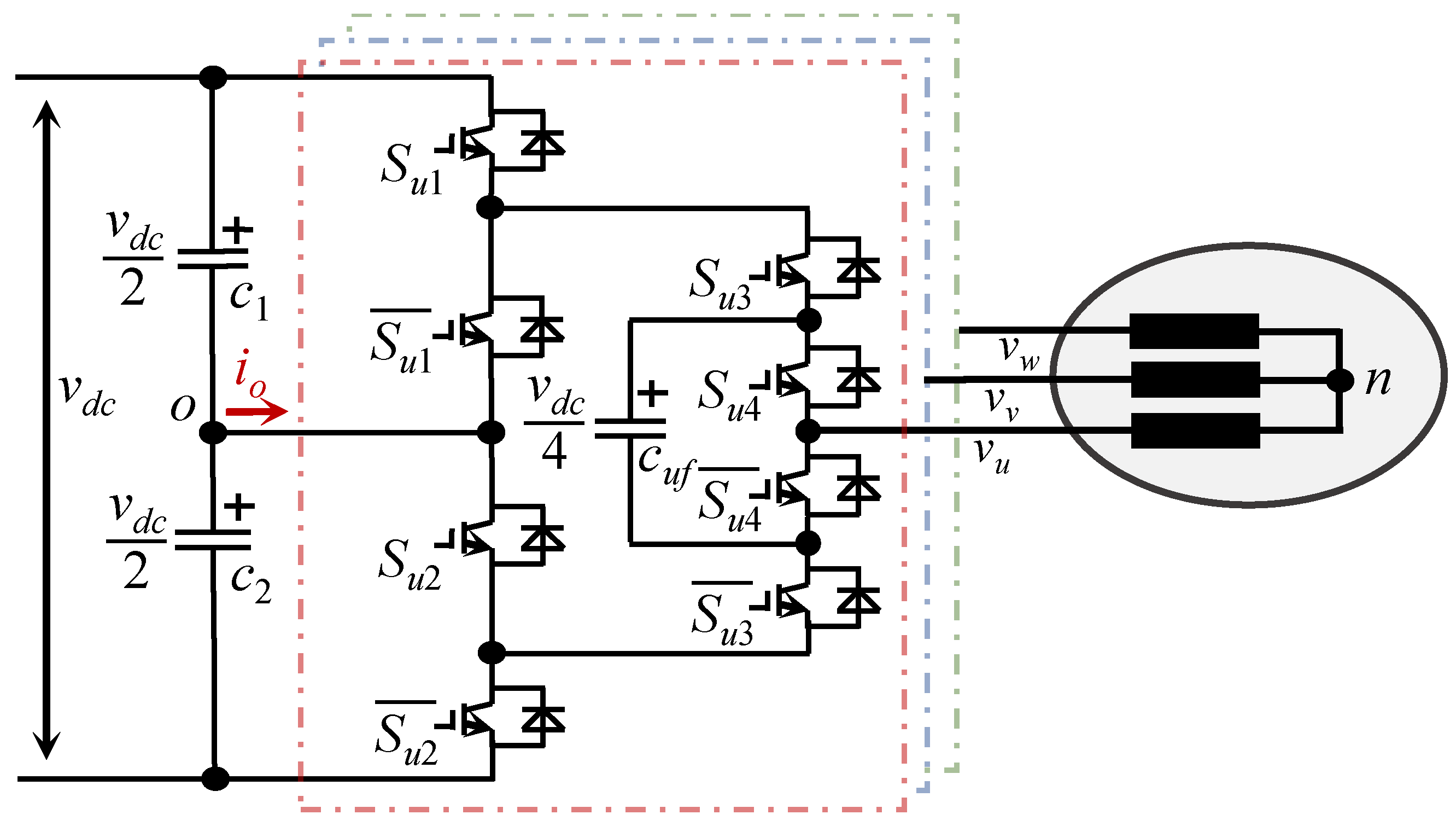
2.1. Principle of Five Level Selective Harmonic Elimination Pulse-Width Modulation
2.2. Mechanism of Common-Mode Voltage Problem under Selective Harmonic Elimination Pulse-Width Modulation
3. Analysis of Multimode Characteristics in Five-Level Selective Harmonic Elimination Pulse-Width Modulation and Discussion on Their Corresponding Common-Mode Voltage
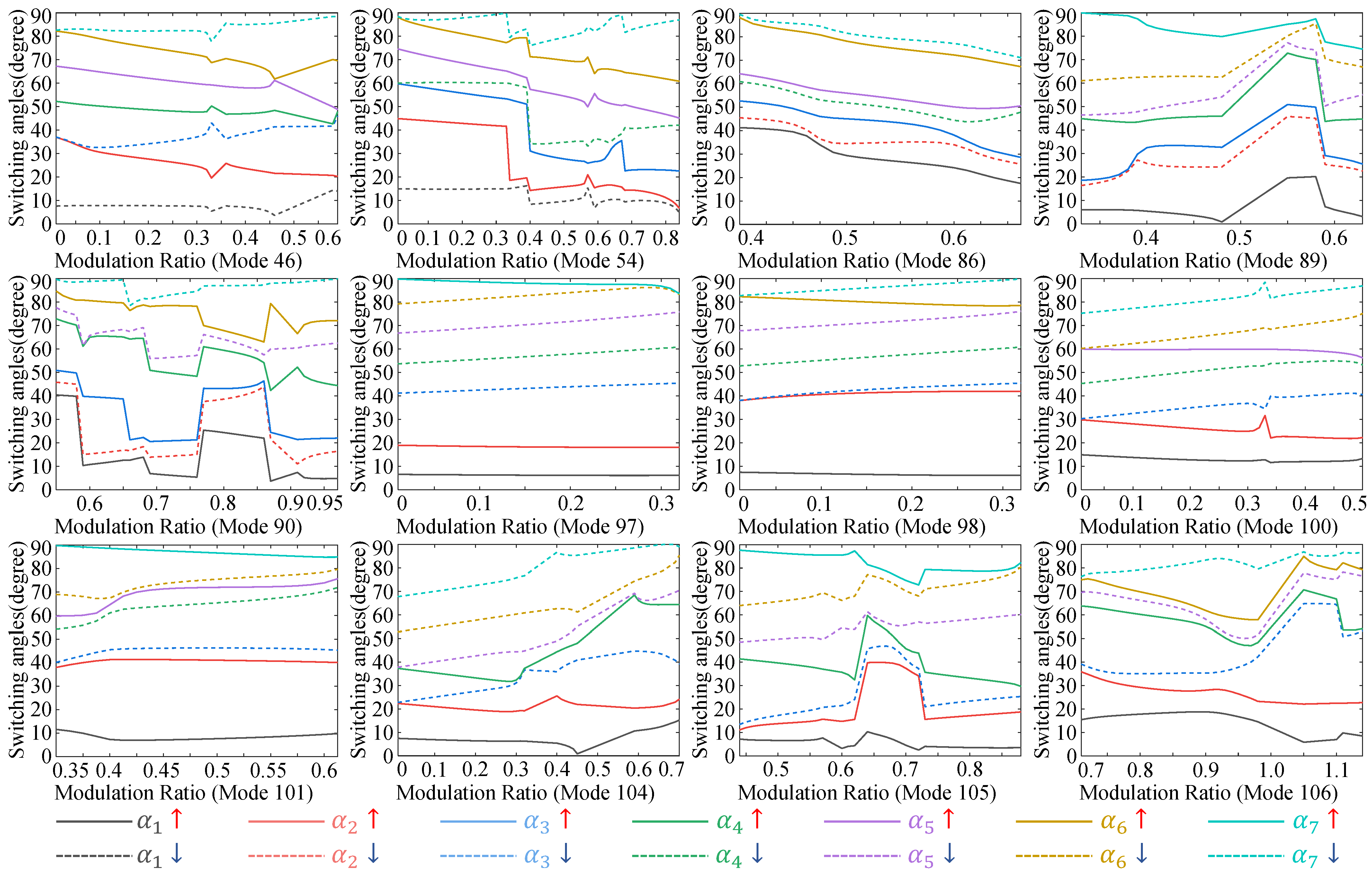
3.1. Multimode in Five-Level Selective Harmonic Elimination Pulse-Width Modulation
- Random search: Although the initial value calculation method of the equal area method under five-level SHEPWM has been studied, it is not suitable for the five-level multimode case. At multiple levels, there are multiple switching angle solutions from multiple modes or multiple switching angles within one mode under one modulation ratio. Fortunately, under the uniform constraint formula (8), the probability of obtaining the switching angle solution is very high with a set of random initial values from 0 to . So, for one modulation ratio, it is necessary to carry out several random value calculation processes to find a complete switching angle solution under the modulation ratio as much as possible. In the random search phase, most angle solutions can be obtained efficiently for the full modulation ratio of each mode. At the same time, the greater the number of search (NS) times under one modulation ratio, the higher the possibility of obtaining a complete solution is, but the lower the search efficiency. A mere random search is a purposeless search, which is suitable for the first stage of the full solution space search.
- Endpoints’ replenishment: According to the continuity feature of the SHEPWM switching angle solution trajectory, there is a high probability that a solution exists near the endpoint to form a continuous solution trajectory. The endpoint is defined as the switching angle solution (), where the nearby angle solution, () or (), is not found. The value of 0.01 refers to the search step size of the modulation ratio. So, a certain random disturbance in the endpoint superposition is used as the initial value for the NMs, which is as in (12).where c is the parameter for controlling the magnitude of the random disturbance that takes a value between 0.95 and 1. takes a value between 0 and 1 and sorts them in ascending order. After solving by the fsolve function, the switching angle solution that satisfies the condition is added to the angle solution set. This process is repeated until the endpoints no longer add new angular solutions. The endpoints’ replenishment phase is the process of extending and supplementing the switching angles at the endpoint until the solution trajectory is continuous.
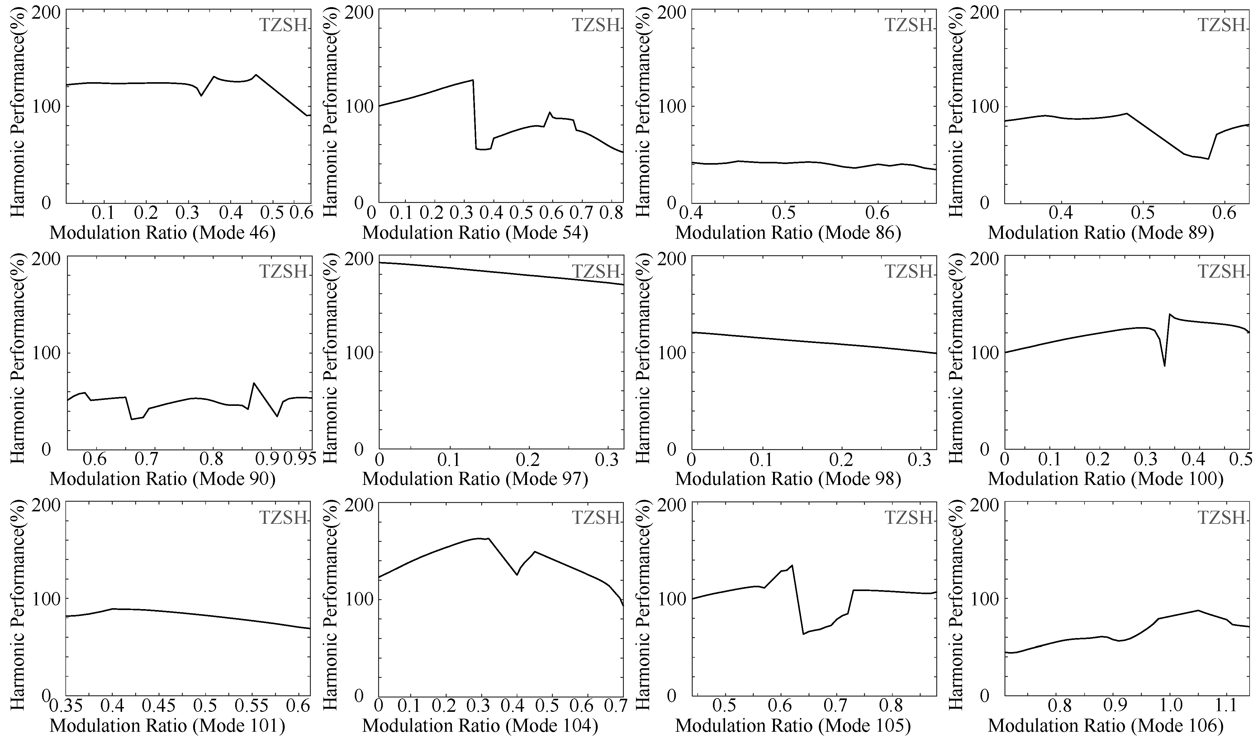
3.2. Common-Mode Voltage and Characteristics under Multiple Modes
4. Optimized-Mode-Trajectory-Based Common-Mode Voltage Suppression Method
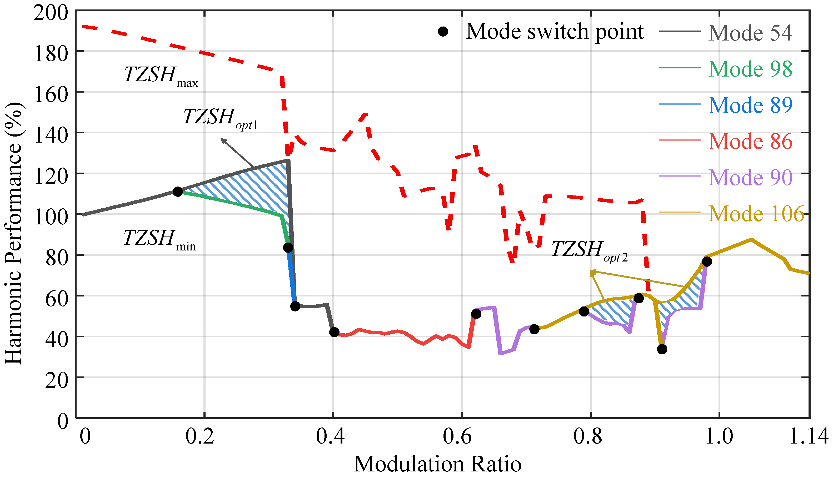
4.1. Optimized Mode Trajectory
4.2. Discussion on Strengths and Weaknesses
5. Experimental Verification
6. Conclusions
Author Contributions
Funding
Data Availability Statement
Conflicts of Interest
References
- Won, J.; Jalali, G.; Liang, X.; Zhang, C.; Srdic, S.; Lukic, S.M. Auxiliary Power Supply for Medium-Voltage Power Converters: Topology and Control. IEEE Trans. Ind. Appl. 2019, 55, 4145–4156. [Google Scholar]
- Ma, B.; Xu, X.; Wang, K.; Zheng, Z.; Li, Y. A Neutral-Point Potential Balancing Method for a Three-Level Neutral-Point-Clamped Back-to-Back Converter. In Proceedings of the 2019 IEEE Transportation Electrification Conference and Expo, Asia-Pacific (ITEC Asia-Pacific), Seogwipo, Republic of Korea, 8–10 May 2019; IEEE: Piscataway, NJ, USA, 2019; pp. 1–5. [Google Scholar]
- Geyer, T.; Mastellone, S. Model predictive direct torque control of a five-level ANPC converter drive system. IEEE Trans. Ind. Appl. 2012, 48, 1565–1575. [Google Scholar] [CrossRef]
- Lee, H.W.; Jang, S.J.; Lee, K.B. Advanced DPWM Method for Switching Loss Reduction in Isolated DC Type Dual Inverter With Open-End Winding IPMSM. IEEE Access 2023, 11, 2700–2710. [Google Scholar] [CrossRef]
- Kim, J.S.; Kim, D.H.; Lee, J.H.; Lee, J.S. Smooth Pulse Number Transition Strategy Considering Time Delay in Synchronized SVPWM. IEEE Trans. Power Electron. 2022, 38, 2252–2261. [Google Scholar] [CrossRef]
- Steczek, M.; Chudzik, P.; Szeląg, A. Combination of SHE-and SHM-PWM techniques for VSI DC-link current harmonics control in railway applications. IEEE Trans. Ind. Electron. 2017, 64, 7666–7678. [Google Scholar]
- Dahidah, M.S.A.; Konstantinou, G.; Agelidis, V.G. A review of multilevel selective harmonic elimination PWM: Formulations, solving algorithms, implementation and applications. IEEE Trans. Power Electron. 2014, 30, 4091–4106. [Google Scholar]
- Wang, C.; Wang, K.; You, X. Research on synchronized SVPWM strategies under low switching frequency for six-phase VSI-fed asymmetrical dual stator induction machine. IEEE Trans. Ind. Electron. 2016, 63, 6767–6776. [Google Scholar] [CrossRef]
- Arumalla, R.T.; Figarado, S.; Panuganti, K.; Harischandrappa, N. Selective Lower Order Harmonic Elimination in DC-AC Converter Using Space Vector Approach. IEEE Trans. Circuits Syst. II Express Briefs 2021, 68, 2890–2894. [Google Scholar]
- Lak, M.; Chuang, B.R.; Lee, T.L. A common-mode voltage elimination method with active neutral point voltage balancing control for three-level T-type Inverter. IEEE Trans. Ind. Appl. 2022, 58, 7499–7514. [Google Scholar] [CrossRef]
- Vu, H.C.; Lee, H.H. Model-predictive current control scheme for seven-phase voltage-source inverter with reduced common-mode voltage and current harmonics. IEEE J. Emerg. Sel. Top. Power Electron. 2020, 9, 3610–3621. [Google Scholar] [CrossRef]
- Yang, Y.; Wen, H.; Fan, M.; Xie, M.; Peng, S.; Norambuena, M.; Rodriguez, J. Computation-efficient model predictive control with common-mode voltage elimination for five-level ANPC converters. IEEE Trans. Transp. Electrif. 2020, 6, 970–984. [Google Scholar]
- Yang, Y.; Chen, R.; Fan, M.; Xiao, Y.; Zhang, X.; Norambuena, M.; Rodriguez, J. Improved model predictive current control for three-phase three-level converters with neutral-point voltage ripple and common mode voltage reduction. IEEE Trans. Energy Convers. 2021, 36, 3053–3062. [Google Scholar] [CrossRef]
- Yang, Y.; Pan, J.; Wen, H.; Zhang, X.; Norambuena, M.; Xu, L.; Rodriguez, J. Computationally efficient model predictive control with fixed switching frequency of five-level ANPC converters. IEEE Trans. Ind. Electron. 2021, 69, 11903–11914. [Google Scholar] [CrossRef]
- Xu, X.; Wang, K.; Zheng, Z.; Li, Y. A simple common-mode voltage reduction method based on zero-sequence voltage injection for a back-to-back three-level NPC converter. In Proceedings of the 2021 IEEE Energy Conversion Congress and Exposition (ECCE), Vancouver, BC, Canada, 10–14 October 2021; IEEE: Piscataway, NJ, USA, 2021; pp. 3228–3233. [Google Scholar]
- Qin, C.; Li, X.; Xing, X.; Zhang, C.; Zhang, G. Common-mode voltage reduction method for three-level inverter with unbalanced neutral-point voltage conditions. IEEE Trans. Ind. Inform. 2020, 17, 6603–6613. [Google Scholar] [CrossRef]
- Chen, J.; Jiang, D.; Sun, W.; Pei, X. Common-mode voltage reduction scheme for MMC with low switching frequency in AC–DC power conversion system. IEEE Trans. Ind. Inform. 2021, 18, 278–287. [Google Scholar]
- Sadoughi, M.; Pourdadashnia, A.; Farhadi-Kangarlu, M.; Galvani, S. PSO-optimized SHE-PWM technique in a cascaded H-bridge multilevel inverter for variable output voltage applications. IEEE Trans. Power Electron. 2022, 37, 8065–8075. [Google Scholar] [CrossRef]
- Jiang, Y.; Li, X.; Qin, C.; Xing, X.; Chen, Z. Improved particle swarm optimization based selective harmonic elimination and neutral point balance control for three-level inverter in low-voltage ride-through operation. IEEE Trans. Ind. Inform. 2021, 18, 642–652. [Google Scholar] [CrossRef]
- Fei, W.; Du, X.; Wu, B. A generalized half-wave symmetry SHE-PWM formulation for multilevel voltage inverters. IEEE Trans. Ind. Electron. 2009, 57, 3030–3038. [Google Scholar]
- Perez-Basante, A.; Ceballos, S.; Konstantinou, G.; Pou, J.; Kortabarria, I.; de Alegría, I.M. A universal formulation for multilevel selective-harmonic-eliminated PWM with half-wave symmetry. IEEE Trans. Power Electron. 2018, 34, 943–957. [Google Scholar]
- Perez-Basante, A.; Ceballos, S.; Konstantinou, G.; Pou, J.; Andreu, J.; de Alegría, I.M. (2N+ 1) selective harmonic elimination-PWM for modular multilevel converters: A generalized formulation and a circulating current control method. IEEE Trans. Power Electron. 2017, 33, 802–818. [Google Scholar] [CrossRef]
- Xin, Y.; Yi, J.; Zhang, K.; Chen, C.; Xiong, J. Offline selective harmonic elimination with (2N+ 1) output voltage levels in modular multilevel converter using a differential harmony search algorithm. IEEE Access 2020, 8, 121596–121610. [Google Scholar] [CrossRef]
- Tripathi, A.; Narayanan, G. Torque ripple minimization in neutral-point-clamped three-level inverter fed induction motor drives operated at low-switching-frequency. IEEE Trans. Ind. Appl. 2018, 54, 2370–2380. [Google Scholar]
- Guan, B.; Doki, S. A current harmonic minimum PWM for three-level converters aiming at the low-frequency fluctuation minimum of neutral-point potential. IEEE Trans. Ind. Electron. 2018, 66, 3380–3390. [Google Scholar]
- Wu, M.; Xue, C.; Li, Y.W.; Yang, K. A generalized selective harmonic elimination PWM formulation with common-mode voltage reduction ability for multilevel converters. IEEE Trans. Power Electron. 2021, 36, 10753–10765. [Google Scholar] [CrossRef]
- Sharifzadeh, M.; Babaie, M.; Chouinard, G.; Al-Haddad, K.; Portillo, R.; Franquelo, L.G.; Gopakumar, K. Hybrid SHM-PWM for common-mode voltage reduction in three-phase three-level NPC inverter. IEEE J. Emerg. Sel. Top. Power Electron. 2020, 9, 4826–4838. [Google Scholar] [CrossRef]
- Sharifzadeh, M.; Sadabadi, M.S.; Laurendeau, E.; Al-Haddad, K. Multi-objective SHM-PWM modulation technique for CMV control in 3-phase inverters. In Proceedings of the 2023 IEEE 32nd International Symposium on Industrial Electronics (ISIE), Helsinki, Finland, 19–21 June 2023; IEEE: Piscataway, NJ, USA, 2023; pp. 1–6. [Google Scholar]


| Methods | Levels Studied | Modulation | Switching Frequency | CMV | THD |
|---|---|---|---|---|---|
| voltage vector with low CMV [12,13,14] | three and multi-level | SVPWM and MPC | high | low | medium |
| zero-sequence voltage injection [15,16] | three level | SPWM | high | low | medium |
| voltage vector with zero CMV [17] | multi-level | NZCMVV | low | zero | high |
| harmonic elimination or mitigation [26,27,28] | three-level | SHEPWM and SHMPWM | low | low | low |
| Level | 2 | 1 | 1 | 0 | 0 | −1 | −1 | −2 |
|---|---|---|---|---|---|---|---|---|
| on | on | on | on | off | off | off | off | |
| on | on | on | on | off | off | off | off | |
| on | on | off | off | on | off | on | off | |
| on | off | on | off | on | on | off | off |
| m | 0.1 | 0.2 | 0.3 | 0.4 | 0.5 | 0.6 | 0.7 | 0.8 | 0.97 |
|---|---|---|---|---|---|---|---|---|---|
| case 1 | 1.06 (54) | 1.09 (98) | 1.01 (98) | 0.42 (86) | 0.43 (86) | 0.36 (86) | 0.44 (90) | 0.51 (90) | 0.54 (90) |
| case 2 | 1.10 (100) | 1.15 (54) | 1.22 (46) | 0.66 (54) | 0.77 (54) | 0.52 (90) | 0.73 (54) | 0.55 (106) | 0.73 (106) |
| case 3 | 1.15 (98) | 1.20 (100) | 1.24 (54) | 0.88 (89) | 0.80 (101) | 0.75 (89) | 0.79 (105) | 0.57 (54) | |
| case 4 | 1.24 (46) | 1.24 (46) | 1.25 (100) | 0.89 (101) | 1.08 (105) | 0.88 (54) | 0.93 (104) | 1.08 (105) | |
| case 5 | 1.39 (104) | 1.54 (104) | 1.63 (104) | 1.25 (104) | 1.20 (100) | 1.26 (104) | |||
| case 6 | 1.87 (97) | 1.79 (97) | 1.71 (97) | 1.26 (46) | 1.29 (105) | ||||
| case 7 | 1.31 (100) |
| N-Feature | Range 1 | Range 2 | Range 3 | Range 4 | Range 5 |
|---|---|---|---|---|---|
| 5- | |||||
| 5-mode | mode 14 | mode 22 | mode 25 | mode 26 | |
| 7- | |||||
| 7-mode | mode 54 | mode 86 | mode 90 | mode 106 | |
| 9- | |||||
| 9-mode | mode 402 | mode 214 | mode 342 | mode 346 | mode 362 |
| Parameters | Experiment Value |
|---|---|
| DC-link voltage () | 180 V |
| Upper and bottom capacitor () | mF |
| Flying capacitor () | mF |
| Base frequency (BF) | 50 Hz |
| R-load | 20 |
| -load | 30 mH |
| Mode | TZSH | ||||||||
|---|---|---|---|---|---|---|---|---|---|
| 0.2 | 97 | 1.790 | 6.0907 | 18.1079 | 43.8777 | 57.8349 | 71.7076 | 84.0559 | 87.7112 |
| 54 | 1.153 | 14.7970 | 42.8632 | 55.7531 | 60.2542 | 68.6148 | 81.0791 | 87.8051 | |
| 0.5 | 100 | 1.204 | 13.2686 | 22.2327 | 40.482 | 53.1922 | 56.2091 | 75.1309 | 86.9406 |
| 86 | 0.426 | 27.8713 | 34.7755 | 44.3154 | 50.6552 | 54.6971 | 76.2578 | 79.9691 | |
| 0.66 | 104 | 1.141 | 12.6403 | 21.3068 | 43.236 | 64.3369 | 67.6133 | 78.8194 | 89.9732 |
| 90 | 0.316 | 12.5836 | 16.6783 | 21.263 | 64.2222 | 67.4298 | 76.4245 | 78.5191 | |
| 0.85 | 105 | 1.058 | 3.4746 | 18.1354 | 24.6972 | 31.4997 | 59.4013 | 76.1961 | 79.0356 |
| 106 | 0.588 | 18.4544 | 27.864 | 35.218 | 58.2564 | 63.5534 | 66.6092 | 80.8947 |
| Mode | (V) | TZSH | CMV(V) | Current THD (%) | |
|---|---|---|---|---|---|
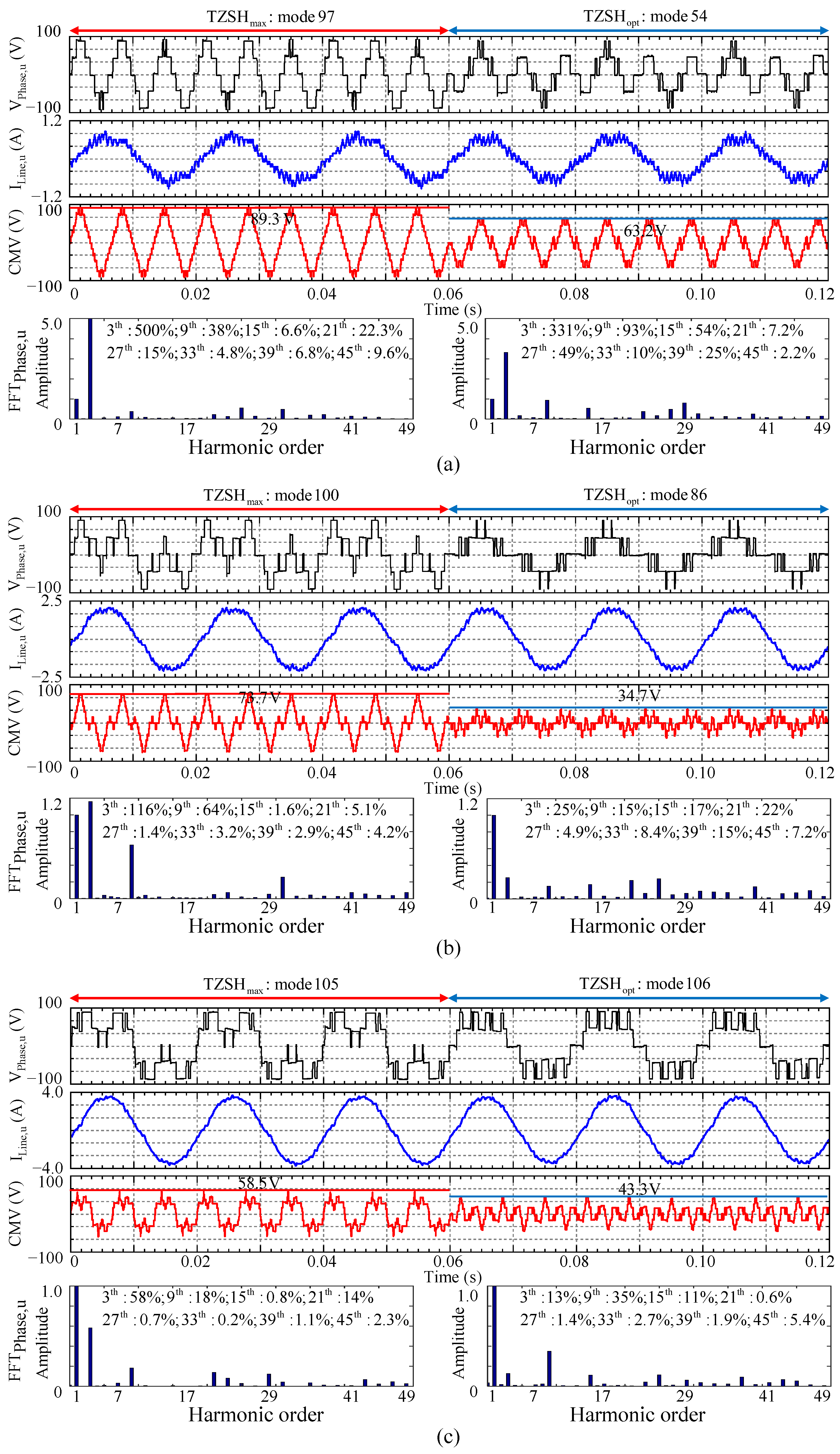
| [0.2, 17.2 V] | 97 | [16.58, 0.62] | 1.740 | 89.3 | 16.78 |
| 54 | [15.62, 1.58] | 1.146 (⇓34.1%) | 63.2 (⇓29.2%) | 20.78 (⇑23.8%) | |
| [0.5, 43 V] | 100 | [42.3, 0.7] | 1.247 | 73.7 | 7.83 |
| 86 | [41.8, 1.2] | 0.418 (⇓66.5%) | 34.7 (⇓53.0%) | 7.26 (⇓7.3%) | |
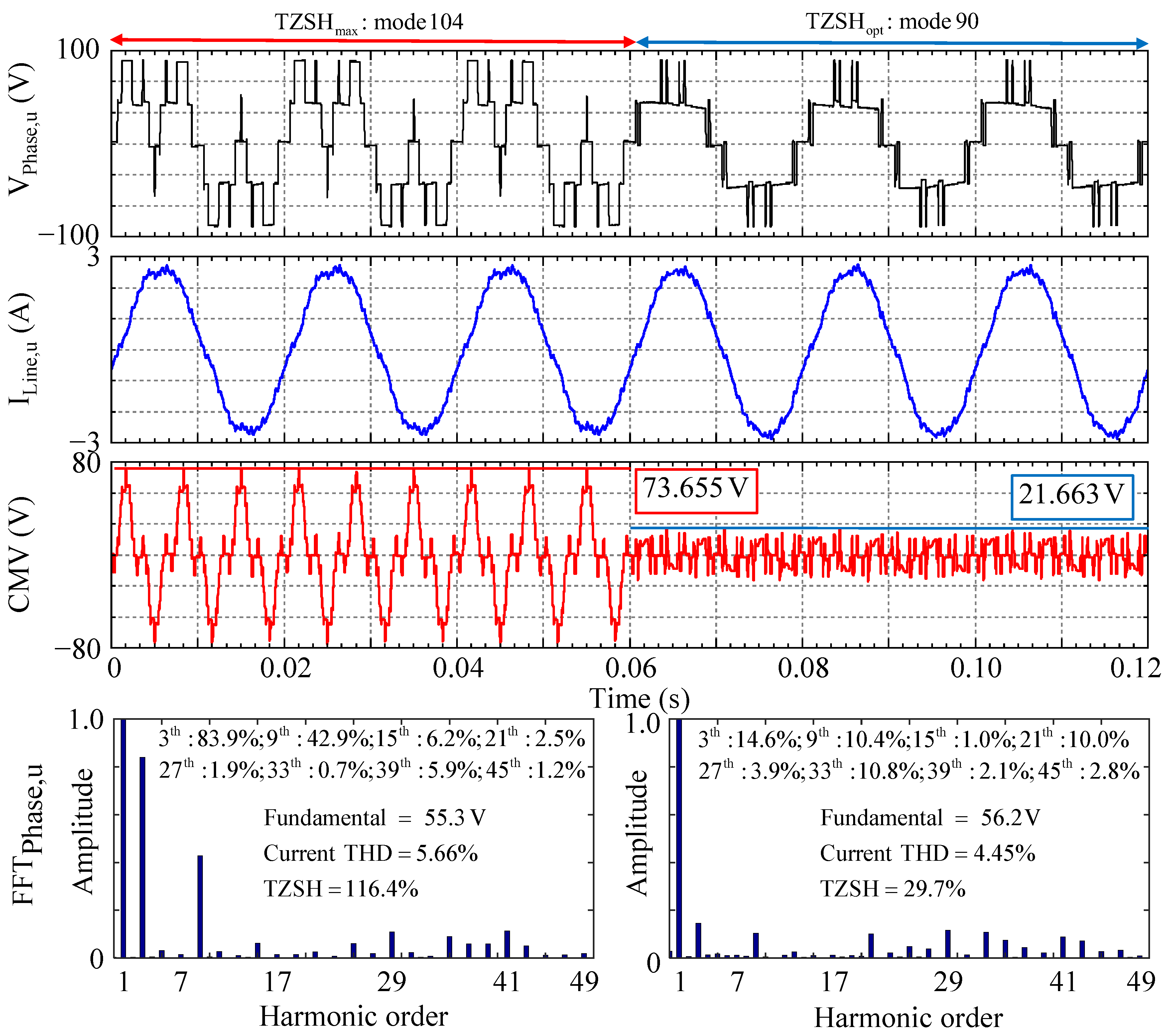
| [0.66, 56.7 V] | 104 | [55.3, 1.4] | 1.164 | 73.655 | 5.66 |
| 90 | [56.2, 0.5] | 0.297 (⇓74.5%) | 21.663 (⇓70.6%) | 4.45 (⇓21.4%) | |
| [0.85, 73.1 V] | 105 | [72.7, 0.4] | 1.013 | 58.5 | 4.79 |
| 106 | [70.6, 2.5] | 0.617 (⇓39.1%) | 43.3 (⇓26.0%) | 4.26(⇓11.1%) |
Disclaimer/Publisher’s Note: The statements, opinions and data contained in all publications are solely those of the individual author(s) and contributor(s) and not of MDPI and/or the editor(s). MDPI and/or the editor(s) disclaim responsibility for any injury to people or property resulting from any ideas, methods, instructions or products referred to in the content. |
© 2024 by the authors. Licensee MDPI, Basel, Switzerland. This article is an open access article distributed under the terms and conditions of the Creative Commons Attribution (CC BY) license (https://creativecommons.org/licenses/by/4.0/).
Share and Cite
Luo, C.; Guan, B. Common-Mode Voltage Suppression of a Five-Level Converter Based on Multimode Characteristics of Selective Harmonic Elimination PWM. Electronics 2024, 13, 408. https://doi.org/10.3390/electronics13020408
Luo C, Guan B. Common-Mode Voltage Suppression of a Five-Level Converter Based on Multimode Characteristics of Selective Harmonic Elimination PWM. Electronics. 2024; 13(2):408. https://doi.org/10.3390/electronics13020408
Chicago/Turabian StyleLuo, Chuanchuan, and Bo Guan. 2024. "Common-Mode Voltage Suppression of a Five-Level Converter Based on Multimode Characteristics of Selective Harmonic Elimination PWM" Electronics 13, no. 2: 408. https://doi.org/10.3390/electronics13020408
APA StyleLuo, C., & Guan, B. (2024). Common-Mode Voltage Suppression of a Five-Level Converter Based on Multimode Characteristics of Selective Harmonic Elimination PWM. Electronics, 13(2), 408. https://doi.org/10.3390/electronics13020408