Modeling, System Identification, and Control of a Railway Running Gear with Independently Rotating Wheels on a Scaled Test Rig

Abstract

The development and validation of lateral control strategies for railway running gears with independently rotating driven wheels (IRDWs) are an active research area due to their potential to enhance straight-track centering, curve steering performance, and reduce noise and wheel–rail wear. This paper focuses on the practical application of theoretical models to a 1:5 scaled test rig developed by the German Aerospace Center (DLR), addressing the challenges posed by unmodeled phenomena such as hysteresis, varying damping and parameter identification. The theoretical model from prior work is adapted based on empirical measurements from the test rig, incorporating the varying open-loop stability of the front and rear wheel carriers, hysteresis effects, and other dynamic properties typically neglected in literature. A transparent procedure for identifying dynamic parameters is developed, validated through closed- and open-loop measurements. The refined model informs the design and tuning of a cascaded PI and PD controller, enhancing system stabilization by compensating for hysteresis and damping variations. The proposed approach demonstrates improved robustness and performance in controlling the lateral displacement of IRDWs, contributing to the advancement of safety-critical railway technologies.

1. Introduction

Railway running gears with independently rotating driven wheels (IRDWs) have been a prominent research focus over the past decades due to their significant advantages. These include improved straight-track centering, enhanced curve steering performance, and notable reductions in noise and wheel–rail wear. However, these benefits require active control systems, leading to the development of new technologies that are highly safety-relevant and subject to rigorous approval processes. This contrasts with the well-established, simple, and cost-effective passive track guidance systems that have been used for nearly 200 years. With the increasing demands of modern railway systems, particularly the introduction of high-speed and urban light rail vehicles, new approaches and innovations are necessary to address challenges like curving ability and hunting stability at higher speeds [1].

In response to these challenges, the German Aerospace Center (DLR) initiated the internal project “Next Generation Train (NGT)” [2], which explores running gears utilizing independently rotating and driven wheels. In this context, a 1:5 prototype of such a running gear was developed, building on previous research [2,3,4,5]. Roller rigs are widely used in railway vehicle research for their high controllability, repeatability, and flexibility in experiment setups, as well as their lower cost compared to field tests [6]. They are particularly valuable when evaluating the stability properties of independently rotating driven wheels (IRDWs) [7,8,9,10]. The roller rig discussed in this paper is distinctive, featuring motorized actuation for each wheel and incorporating two separate wheel carriers with different stability characteristics, unlike conventional designs that typically employ only one. The main challenges in controlling IRDWs are twofold.

First, the control design itself is challenging due to the complex and difficult-to-model wheel–rail contact. The simplest solution is to mimic the behavior of a traditional wheelset by controlling the angular velocity to zero [11,12]. While this stabilizes the system, it forfeits many of the advantages of IRDWs. The next step is to control the yaw angle to stabilize the system [13]. This can also be achieved passively by altering the wheel tread conicity to a negative value [10]. However, this approach does not allow for precise control of the lateral displacement necessary to reduce wear and noise.

Therefore, the most fundamental control strategy to drive the lateral displacement to a reference value is the use of PID control, as presented in [14]. Despite its simplicity, PID control has limitations in performance and robustness, prompting the exploration of more advanced control strategies such as $H_{\infty }$ control [15,16], semi-active control [17,18], sliding mode control [19], feedback linearization [20], reinforcement learning [21,22], and model predictive control [23].

The second major challenge is accurately acquiring the lateral displacement used for control. Optical sensors, while effective, are prone to interference from dirt, ballast, and weather conditions due to their proximity to the rail bed [21]. Consequently, the use of observers, which estimate the lateral displacement from other measurements such as yaw angle and angular velocity, is investigated. This approach is explored in [5] for different sensor configurations using different versions of Kalman Filters. Simpler observers using less model information are also developed [24]. A key requirement to allow for an observation of the lateral displacement is the non-linearity of the wheel profile. This non-linearity is often characterized by a parameter known as equivalent conicity. While low-fidelity models typically assume a constant equivalent conicity, more advanced designs, such as in [25], employ an observer to estimate this parameter in real time.

For these observers to be effective, the underlying model dynamics must be accurate. The quality of the observer and the design and tuning of the controller are both improved with better underlying models. Although many theoretical models of varying complexity have been proposed for the IRDW system, practical adaptation of these models to the test rig and procedures for parameter transformation have been lacking.

This paper contributes by adapting the model used in previous work [24] based on measurements from the 1:5 test rig. It incorporates commonly neglected properties such as different stability behavior of the wheel carriers, hysteresis effects, and varying damping into the system model. Additionally, a transparent procedure for identifying individual dynamic parameters is developed. Both closed- and open-loop measurements validate the developed model and parameters. Finally, the model is used to design and tune a cascaded PI and PD controller (PI-PD controller) that compensates for hysteresis and varying damping effects.

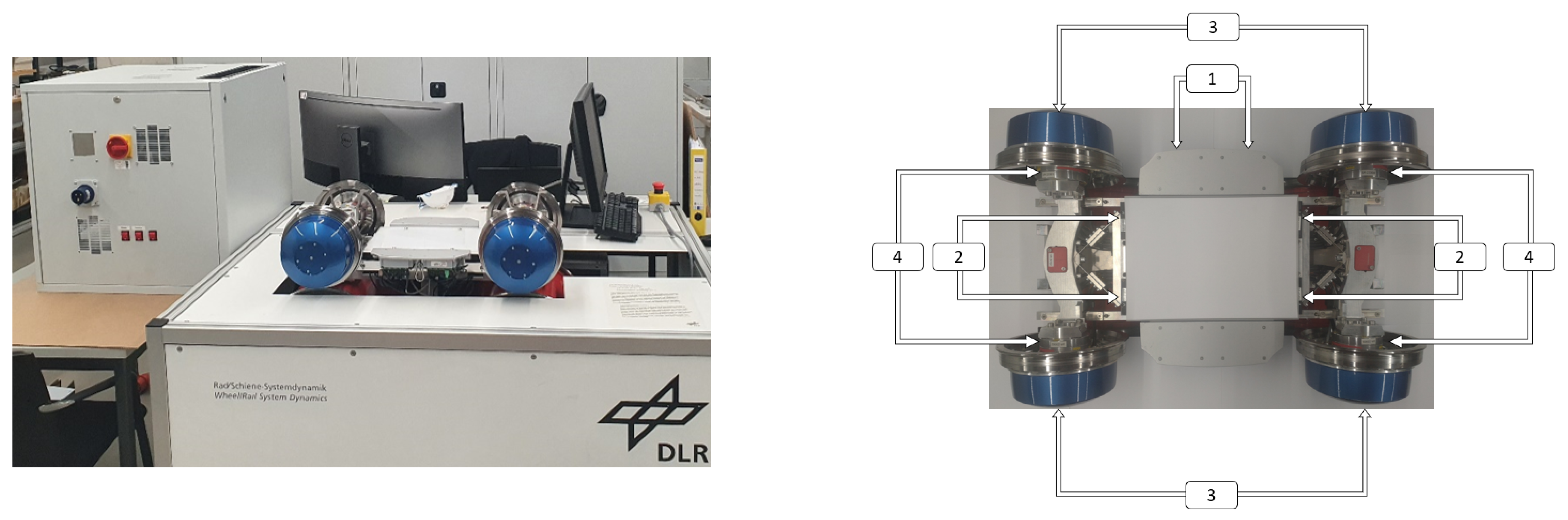
2. System and Sensor Setup

A visual impression of the 1:5 test rig investigated throughout this paper can be found in Figure 1.

The running gear consists of four IRDWs, each independently driven by motors housed within the wheels. These motors are permanently excited synchronous machines, each controlled by its own power converter and provide based on the commanded input current u the required differential torque to steer the system.

Each pair of wheels is connected by an axle bridge, which is coupled to the running gear frame via a leaf spring guidance system that enables the yaw motion of the axle bridges. The running gear is mounted on two revolving rollers, simulating the longitudinal motion of the vehicle.

The test rig is equipped with several sensors for the control and monitoring of the IRDWs as displayed in Figure 1 and Figure 2. First, two laser sensors are mounted on the roller rig frame which measure the distance to two metal plates at the front and rear $b_{\mathrm{f}}/b_{\mathrm{r}}$. These signals can be used to obtain the mean distance $y_{\mathrm{m}}={\displaystyle \frac{b_{\mathrm{f}}+b_{\mathrm{r}}}{2}}-b_0$, where $b_0$ is the nominal lateral distance between the laser sensors and the metal plates if the vehicle centre aligns with the track centre. Further, the angle between frame and rail is $sin\left({\psi }_{\mathrm{m}}\right)={\displaystyle \frac{b_{\mathrm{f}}-b_{\mathrm{r}}}{l_{\mathrm{L}}}}$, where $l_{\mathrm{L}}$ denotes the distance between the front and rear laser sensor. The signals are propagated to obtain the control variables and the lateral displacement of front and rear wheel carrier as

$$\begin{array}{ccc}\hfill y_{\mathrm{f}}=y_{\mathrm{m}}+sin\left({\psi }_{\mathrm{m}}\right)l_0& \hfill & \hfill y_{\mathrm{r}}=y_{\mathrm{m}}-sin\left({\psi }_{\mathrm{m}}\right)l_0\end{array}$$

where $l_0$ defines the distance of front/rear wheel carrier to the middle of the frame.

Second, four laser sensors are mounted at the front left, front right, rear left, and rear right on the running gear frame, measuring the distances to the front/rear wheel carrier $s_{\mathrm{fl}},s_{\mathrm{fr}},s_{\mathrm{rl}},s_{\mathrm{rr}}$. These allow to obtain the angle between frame and front/rear wheel carrier as

$$\begin{array}{ccc}\hfill {\psi }_{\mathrm{af}}=tan\left({\displaystyle \frac{s_{\mathrm{fl}}-s_{\mathrm{fr}}}{d_0}}\right)& \hfill & \hfill {\psi }_{\mathrm{ar}}=tan\left({\displaystyle \frac{s_{\mathrm{rl}}-s_{\mathrm{rr}}}{d_0}}\right)\end{array}$$

where $d_0$ denotes the distance between the left and right laser sensor measuring the yaw angle, respectively.

Third, the angular velocity of the front left, front right, rear left, and rear right wheel ${\omega }_{\mathrm{fl}},{\omega }_{\mathrm{fr}},{\omega }_{\mathrm{rl}},{\omega }_{\mathrm{rr}}$ is measured using encoders mounted inside the wheels.

Finally, each axle bridge is equipped with force-torque sensors mounted on the left and right sides, yielding force torque signals along the $x,y,z$ axis denoted by $F_{ijk}$, $M_{ijk}$ where $i\in \{\mathrm{x},\mathrm{y},\mathrm{z}\}$, $j\in \{\mathrm{f},\mathrm{r}\}$ and $k\in \{\mathrm{l},\mathrm{r}\}$. A sketch illustrating some of these quantities discussed is given in Figure 2 which is analyzed in detail in Section 4.

The running gear hardware is connected to a rapid control prototyping environment. Simulation models are implemented in MATLAB/Simulink 2015b and compiled using the Simulink Real-Time 2015b environment and a sampling time of $h=0.005 \mathrm{s}$. For a more detailed description of the test rig and its technical details, refer to [5].

3. Motivation

To provide an initial insight into the system dynamics, a step input current applied solely to the rear wheels, with the front wheel carrier not in contact with the rollers, is illustrated in Figure 3. This setup yields the yaw angle measurements depicted in Figure 4. The experiment was conducted three times, revealing qualitatively consistent behavior across all trials but with quantitative differences of up to $1\mathrm{rad}$ relative to a total change of $7\mathrm{rad}$. Surprisingly, the measurement signals indicate an open-loop stable system, contrary to expectations from models such as those in [5], in which integrating behavior from yaw angle to lateral displacement is suggested. Moreover, the measurements exhibit unexpected steady-state behavior, where the stationary value for $u=0$ differs before and after $t=300 \mathrm{s}$. Additionally, the step response shown in Figure 4 demonstrates varying dynamics over time. At approximately $t\approx 20 \mathrm{s}$, a significant yaw angle jump occurs, indicative of a system with very small damping. However, beyond $t\approx 20.2 \mathrm{s}$, the convergence to a steady-state value is slow, characteristic of a system with high damping. These observed effects, along with their modeling and parameter identification, are thoroughly discussed in the subsequent sections of this paper.

4. Modeling and System Identification

This section develops the model describing the system dynamics based on models and notation from [24,26]. These foundational models are expanded and their parameters identified using measurements specific to scenarios on the 1:5 test rig. The model encompasses three primary dynamics: lateral, angular velocity, and yaw dynamics for both front and rear wheel carriers, which may not be fully decoupled. Variables for the wheel carriers are denoted with subscripts ${·}_{\mathrm{f}}$ for the front wheel carrier and ${·}_{\mathrm{r}}$ for the rear wheel carrier. Broadly, the dynamics describe how a differential torque $\Delta u$ applied to the wheels induces a differential angular velocity $\Delta \omega$, leading to a yaw angle $\psi$ and subsequently influencing lateral displacement y dependent on velocity v. This mathematical framework, incorporating geometric and physical parameters, is detailed in the remainder of this section. For all tasks regarding the identifications of these parameters, an optimization problem of the form

$$\begin{array}{cccc}& \underset{c}{min}\hfill & \hfill & {\int }_{t_{\mathrm{start}}}^{t_{\mathrm{end}}}{\left|e\left(t\right)\right|}^2\mathrm{d}t\hfill \end{array}$$

(1a)

$$\begin{array}{cc}\mathrm{s}.\mathrm{t}. \hfill & \dot{x}=f\left(x\right)\hfill \end{array}$$

(1b)

$$\begin{array}{cc} \hspace{1em} \hspace{1em} \hfill & x\left(0\right)=x_{\mathrm{meas}}\left(0\right)\hfill \end{array}$$

(1c)

is solved, where $c\in {\mathbb{R}}^{n_c}$ denotes the parameters to be identified, $e\left(t\right)\in {\mathbb{R}}^{n_e}$ is the error vector defined by the states $x\left(t\right)\in {\mathbb{R}}^{n_x}$ obtained from the model and its dynamics f with $f\left(x\left(t\right)\right)\in {\mathbb{R}}^{n_x}$ and the measurements $x_{\mathrm{meas}}\left(t\right)\in {\mathbb{R}}^{n_x}$ obtained from the test rig with $n_c,n_e,n_x\in \mathbb{N}$ and $t,t_{\mathrm{start}},t_{\mathrm{end}}\in {\mathbb{R}}_{\ge 0}$. The optimization is performed using the MOPS (Multi-Objective Parameter Synthesis) software version 6.8 environment, an optimization tool from the Institute of System Dynamics and Control of the German Aerospace Center, as presented in [27]. An overview of all the parameters discussed in the upcoming Section is available in

Table 1. Parameters and constants.

Notation	Description	Nominal	Identified
v	longitudinal velocity	$1 \mathrm{m} \mathrm{s}$−1
$r_0$	wheel radius	$0.1 \mathrm{m}$
b	track width	$0.3 \mathrm{m}$
$l_{\mathrm{L}}$	distance between laser sensors measuring lateral displacement	$0.1535$ $\mathrm{m}$
$b_0$	nominal distance from laser sensors to metal plates	$0.065$ $\mathrm{m}$
$d_0$	distance between laser sensors measuring yaw angle	$0.185$ $\mathrm{m}$
$k_{\tau }$	motor constant	$0.27 \mathrm{N} \mathrm{m} \mathrm{A}$−1
$l_0$	distance wheel carrier and middle frame	$0.25 \mathrm{m}$	$0.28 \mathrm{m}$
${\delta }_0$	equivalent conicity	$0.024 \mathrm{rad}$	$0.050 \mathrm{rad}$
$y_{\mathrm{off}}$	offset lateral displacement	0 $\mathrm{m}$	$-0.0006$ $\mathrm{m}$
$J_x$	wheel inertia w.r.t rolling	$0.027 \mathrm{k}\mathrm{g}{\mathrm{m}}^2$
${\overline{c}}_{11}$	extended Kalker friction coefficient	$3.6\times {10}^4$ $\mathrm{N} \mathrm{rad}$−1	$3.85\times {10}^4$ $\mathrm{N} \mathrm{rad}$−1
${\omega }_{\mathrm{off}}$	offset angular velocity	0 $\mathrm{rad}$ $\mathrm{s}$−1	$-0.002$ $\mathrm{rad}$ $\mathrm{s}$−1
$J_z$	axle bridge inertia w.r.t yawing	$0.8$ $\mathrm{k}$$\mathrm{g}$$\mathrm{m}$2	$0.28$ $\mathrm{k}$$\mathrm{g}$$\mathrm{m}$2
$k_c$	equivalent stiffness	$66.0$ $\mathrm{N}$ $\mathrm{m}$−1	$98.8$ $\mathrm{N}$ $\mathrm{m}$−1
$k_d$	equivalent damping	$0.66$ $\mathrm{N}$ $\mathrm{s}$ $\mathrm{m}$−1	$21.0$ $\mathrm{N}$ $\mathrm{s}$ $\mathrm{m}$−1
${\psi }_{\mathrm{off}}$	offset yaw angle	0 $\mathrm{rad}$	$-1.8\times {10}^{-3}$$\mathrm{rad}$

. The table includes nominal values used in previous work [5] and identified values resulting from the optimizations conducted in this study. Parameters without identified values retain their nominal values, indicating undetermined aspects in the proposed model. Additionally,

Table 2. Constraints.

Variables	Description	Value
y	lateral displacement	$[-3.5,3.5]$ $\mathrm{m}$$\mathrm{m}$
$\psi$	yaw angle	$[-0.03,0.03]$ $\mathrm{rad}$
$\omega$	angular velocity	$[-41,41]$ $\mathrm{rad}$ $\mathrm{s}$−1
$\Delta u$	current input	$[-4,4]$ $\mathrm{A}$

shows constraints arising for some of the state variables and the input due to physical or security limits. The following sections detail the modeling and parameter identification processes for lateral dynamics, angular velocity dynamics, and yaw dynamics.

4.1. Lateral Dynamics

Beginning with the lateral dynamics, these components are crucial for the control task and are presented herein in a form that is both straightforward to model and allows for easy identification of parameters while still capturing the complexities of real-world dynamics.

4.1.1. Modeling

The model of the lateral dynamics is derived following the approach in [24,26], utilizing linearization, small-angle approximations, and the assumption of no side slip. While the no side-slip assumption may be compromised in real-world applications due to factors such as bad weather, debris, or leaves on the rail, it is justified under the controlled laboratory conditions of this study. This assumption allows for the design, identification, and validation of a model that minimizes the need for frequent online parameter adjustments. The model takes the form

$$\begin{array}{ccc}\hfill {\dot{y}}_{\mathrm{f}}={\overline{c}}_{y}v{\psi }_{\mathrm{f}}& \hfill & \hfill {\dot{y}}_{\mathrm{r}}={\overline{c}}_{y}v{\psi }_{\mathrm{r}}\end{array}$$

where $y_{\mathrm{f}}/y_{\mathrm{r}}$ is the front/rear lateral displacement, ${\psi }_{\mathrm{f}}$/ ${\psi }_{\mathrm{r}}$ is the angle between the rail and the front/rear wheel carrier normal, and v is the velocity. The parameter accounting for the non-flatness of the wheel is denoted by ${\overline{c}}_y$ which is defined as ${\overline{c}}_y={\displaystyle \frac{(2r_{0}cos{\left({\delta }_0\right)}^3-2r_{0}cos\left({\delta }_0\right)+bcos{\left({\delta }_0\right)}^{2}sin\left({\delta }_0\right))}{bsin\left({\delta }_0\right)}}$, where b is the track width, $r_0$ is the wheel radius, and ${\delta }_0$ is the equivalent conicity.

The angles ${\psi }_{\mathrm{f}}$/${\psi }_{\mathrm{r}}$ result from the superposition of ${\psi }_{\mathrm{af}}$/${\psi }_{\mathrm{ar}}$, which is the angle between the wheel carrier and the frame, and ${\psi }_{\mathrm{m}}$, the angle between the frame and the rail, expressed as ${\psi }_{\mathrm{f}}={\psi }_{\mathrm{af}}+{\psi }_{\mathrm{m}}$ illustrated in Figure 2. Laser sensors measure ${\psi }_{\mathrm{af}}$/${\psi }_{\mathrm{ar}}$, while ${\psi }_{\mathrm{m}}$ can be expressed as a function of the lateral displacement,

$$\begin{array}{c}\hfill {\psi }_{\mathrm{m}}=tan\left({\displaystyle \frac{y_{\mathrm{f}}-y_{\mathrm{r}}}{2l_0}}\right)\approx {\displaystyle \frac{y_{\mathrm{f}}-y_{\mathrm{r}}}{2l_0}}\end{array}$$

where $2l_0$ is the distance between the front and rear wheel carrier. Thus, the dynamics take the form

$$\begin{array}{cc}\hfill {\dot{y}}_{\mathrm{f}}& =+{\displaystyle \frac{{\overline{c}}_y}{2l_0}}v{y}_{\mathrm{f}}-{\displaystyle \frac{{\overline{c}}_y}{2l_0}}v{y}_{\mathrm{r}}+{\overline{c}}_{y}v{\psi }_{\mathrm{af}}\hfill \end{array}$$

(2a)

$$\begin{array}{cc}\hfill {\dot{y}}_{\mathrm{r}}& =-{\displaystyle \frac{{\overline{c}}_y}{2l_0}}v{y}_{\mathrm{r}}+{\displaystyle \frac{{\overline{c}}_y}{2l_0}}v{y}_{\mathrm{f}}+{\overline{c}}_{y}v{\psi }_{\mathrm{ar}}.\hfill \end{array}$$

(2b)

It can be seen that considering ${\psi }_{\mathrm{af}}$ as input and for positive velocity $v>0$ and constant rear displacement $y_{\mathrm{r}}=0$, the uncontrolled lateral dynamics at the front wheel carrier (2a) are unstable since ${\displaystyle \frac{v{\overline{c}}_y}{2l_0}}>0$. Conversely, with the same reasoning, the rear wheel carrier dynamics (2b) are stable. Both of these properties become inverted if $v<0$. This is an observation that is rarely discussed in current literature and significantly influences parameter identification, control, and observer design. Identifying an open-loop stable system is inherently easier since it does not necessitate control for obtaining measurements during system identification. Therefore, the method proposed in this work focuses on separately identifying the two wheel carriers. For the rear wheel carrier, this entails conducting measurements under $v>0$ with the front wheel carrier unactuated and lacking roller contact. These measurements allow for the identification of parameters in the lateral dynamics (2b) where $y_{\mathrm{f}}\left(t\right)=0$ for all t. Similarly, the yaw and angular velocity dynamics of the rear wheel carrier can be independently identified, which is detailed in the next section. The same approach applies for identifying the front wheel carrier dynamics under $v<0$. In this work, however, we restrict ourselves on presenting the modeling, system identification, and control of the rear wheel carrier for $v=1 \mathrm{m} \mathrm{s}$⁻¹. Analysis of the unstable case and integration of both wheel carriers will be explored in future studies. To enhance readability, variables $y_{\mathrm{r}}$, ${\psi }_{\mathrm{ar}}$, and $\Delta {\omega }_{\mathrm{r}}$ are denoted without subscripts ${·}_{\mathrm{r}}$ and ${·}_{\mathrm{ar}}$ in the remainder of this work.

4.1.2. Parameter Identification

Augmenting dynamics (2b) by adding a constant offset $y_{\mathrm{off}}$ in the form of ${\displaystyle \frac{v}{2l_0}}{y}_{\mathrm{off}}$ to the right hand side compensating calibration and misalignment errors allows to obtain a good model of the lateral dynamics. Using the input $\Delta u$ from Figure 3 as discussed in Section 3 leads to one measurement with the yaw angle presented in Figure 4 and the lateral displacement shown in Figure 5. For comparison, dynamics (2b) are simulated with the measured yaw angle $\psi ={\psi }_{\mathrm{meas}}$, the nominal parameters from Table 1, and an optimized offset $y_{\mathrm{off}}$. The result is also displayed in Figure 5. It can be seen that this nominal trajectory follows the measurement pretty well and the error is most of the time smaller than the actual measurement noise. However, in particular at the end of the measurement, the error becomes quite large, which motivates the optimization of these theoretical parameters. Velocity v is well known and widely used throughout the model, and parameter ${\delta }_0$ in ${\overline{c}}_y$ is obtained from the optimization in Section 4.2. This leaves the offset $y_{\mathrm{off}}$ and the length $l_0$ as the optimization parameters. The variation of the latter is to be seen as compensating potential alignment errors and model uncertainties. Thus, we consider optimization problem (1) with parameters $c=(y_{\mathrm{off}},l_0)$ with measured lateral displacement $y_{\mathrm{meas}}$, error $e=y_{\mathrm{meas}}-y$, and lateral displacement y subject to dynamics (2b). This leads to the identified parameters displayed in Table 1 which remain reasonably close to the nominal parameters. The simulated results are also displayed in Figure 5. It can be seen that the errors are smaller throughout the entire simulation horizon compared to the nominal simulation.

4.2. Angular Velocity Dynamics

The angular velocity dynamics represent the input–output relationship between the differential input current $\Delta u$ and angular velocity. These dynamics also encompass the motor behavior, which is inherently nonlinear and presents a significant challenge for both modeling and control—a complex research topic in its own right. Modeling the interaction between the rail and wheel is another intricate task. The two main models in this area are the Kalker model, based on linear Kalker theory [28], and the Polach model [29]. While the Polach model is more accurate and accounts for adhesion limits, the Kalker model is linear and computationally efficient. In this work, we adopt the latter to generate a simple linear model, as in [24], which takes the following form:

$$\begin{array}{c}\hfill \Delta \dot{\omega }={\displaystyle \frac{b{\overline{c}}_{11}}{2J_x}}\Gamma y+{\displaystyle \frac{b{\overline{c}}_{11}{r}_0}{2J_{x}v}}\dot{\psi }-{\displaystyle \frac{{\overline{c}}_{11}{r}_0^2}{J_{x}v}}\Delta \omega +{\displaystyle \frac{1}{J_x}}{k}_{\tau }\Delta u\end{array}$$

(3)

where ${\overline{c}}_{11}$ denotes the extended Kalker friction coefficient [26,30], $J_x$ is the inertia of the wheels with respect to rolling, $k_{\tau }$ is the motor constant, and $\Gamma ={\displaystyle \frac{tan\left({\delta }_0\right)}{\frac{b}{2}-r_{0}tan\left({\delta }_0\right)}}$ is a geometric parameter. By employing the nominal parameters from Table 1, it can be seen that the angular velocity dynamics are much faster compared to the lateral and yaw dynamics. Thus, it is sensible to assume the angular velocity dynamics to be in steady state $\Delta \dot{\omega }=0$, i.e., as in [24], the angular velocity can be obtained as

$$\begin{array}{cc}\hfill \Delta \omega & ={\displaystyle \frac{\Gamma vb}{2r_0^2}}y+{\displaystyle \frac{b}{2r_0}}\dot{\psi }+{\displaystyle \frac{v}{r_0^2{\overline{c}}_{11}}}{k}_{\tau }\Delta u.\hfill \end{array}$$

(4)

This relation (4) is sufficient and can replace dynamics (3) as can be seen in the next section. Additionally, it can be used as shown in [24] to design an observer which estimates the lateral displacement based on the input, yaw angle, and angular velocity.

Identification

In order to identify the parameters in Equation (4), the angular velocity measurements for one of the open-loop measurements introduced in Section 3 are used and displayed in Figure 6. It can be seen that the raw measurements admit a very bad ratio from unmodeled dynamics to actual modeled dynamics defined by the lateral displacement, yaw angle, and input. However, by introducing a simple forward–backward low-pass filter with edge frequency of $0.5\mathrm{Hz}$, it is possible to reduce the effect of the unmodeled dynamics. For parameter identification, the raw measurements are used, and the right hand-side of (4) is augmented by offset $\Delta {\omega }_{\mathrm{off}}$. Optimization problem (1) for $c=({\delta }_0,{\overline{c}}_{11},\Delta {\omega }_{\mathrm{off}})$, $e=\Delta {\omega }_{\mathrm{meas}}-\Delta \omega$ is solved where $\Delta \omega$ is obtained by (4) and using the measurements for the right hand-side variables, i.e., $y=y_{\mathrm{meas}}$ and $\dot{\psi }={\displaystyle \frac{{\psi }_{\mathrm{meas}}(k+1)-{\psi }_{\mathrm{meas}}\left(k\right)}{h}}$. The optimization results can be found in Table 1, and the simulated signal $\Delta \omega$ and its filtered version are displayed in Figure 6. It can be seen that the simulation results closely match the measured values. Among the identified parameters, the equivalent conicity angle ${\delta }_0$ is particularly crucial as it significantly impacts the accuracy of lateral displacement estimation, as discussed in [24]. The identified angle is approximately double the nominal value, influenced by factors such as wear, design variations, and assembly inaccuracies affecting the wheel profile. More importantly, the equivalent conicity, following [30], establishes an approximate relationship between differences in rolling radius and lateral displacement amplitude during hunting motion. In Equation (4), this parameter plays a pivotal role, accommodating other potential unmodeled influences through optimization. Conversely, parameter ${\overline{c}}_{11}$ in Equation (4) governs the input’s effect on $\Delta \omega$, though its impact is relatively minor compared to lateral displacement and yaw rate. Consequently, optimization outcomes exhibit notable variability based on initial values and dataset choices, yet the identified parameter remains close to its nominal value.

4.3. Yaw Dynamics

The yaw dynamics play a pivotal role in driving the lateral dynamics and prove to be the most difficult to capture among all dynamics discussed in this work.

4.3.1. Modeling

As given in [24], the dynamics of the yaw angle can be written as

$$\begin{array}{c}\hfill \ddot{\psi }=-{\displaystyle \frac{b^2{\overline{c}}_{11}}{2J_z{r}_0}}\Gamma y+{\displaystyle \frac{-k_{\mathrm{c}}}{J_z}}\psi -\left({\displaystyle \frac{k_{\mathrm{d}}}{J_z}}+{\displaystyle \frac{b^2{\overline{c}}_{11}}{2J_{z}v}}\right)\dot{\psi }+{\displaystyle \frac{b{\overline{c}}_{11}{r}_0}{J_{z}v}}\Delta \omega \end{array}$$

(5)

with $J_{\mathrm{z}}$ being the inertia of the axle bridge with respect to yawing, $k_{\mathrm{c}}$ is the equivalent stiffness, and $k_{\mathrm{d}}$ is the equivalent damping. The use the assumption of fast angular velocity dynamics allows to substitute (4) into the yaw dynamics, which leads to a simple standard second-order system

$$\begin{array}{c}\hfill \ddot{\psi }=-{\displaystyle \frac{k_{\mathrm{c}}}{J_z}}\psi -{\displaystyle \frac{k_{\mathrm{d}}}{J_z}}\dot{\psi }+{\displaystyle \frac{b}{r_0{J}_z}}{k}_{\tau }\Delta u.\end{array}$$

Based on the measurements observed in Figure 4 discussed in Section 3, it is evident that this linear model does not cover all relevant dynamics. Thus, an additional constant offset parameter ${\psi }_{\mathrm{off}}$ accounting for calibration and misalignment errors, a new state $z_{\mathrm{hyst}}$, and a non-linear term accounting for hysteresis $f_{\mathrm{hyst}}(\dot{\psi },z_{\mathrm{hyst}})$ and a different set of parameters ${\omega }_0=\sqrt{{\displaystyle \frac{k_c}{J_{\mathrm{z}}}}}$, $D={\displaystyle \frac{k_{\mathrm{d}}}{2J_{\mathrm{z}}{\omega }_0}}$, $K={\displaystyle \frac{b}{r_0{J}_z{\omega }_0^2}}{k}_{\tau }$ to allow for a simple interpretation of steady state and transitional phase is introduced. Then, the dynamics have the form

$$\begin{array}{c}\hfill \ddot{\psi }=-2D{\omega }_0\dot{\psi }-{\omega }_0^2\psi +K{\omega }_0^2\Delta u+{\omega }_0^2{\psi }_{\mathrm{off}}+f_{\mathrm{hyst}}(\dot{\psi },z_{\mathrm{hyst}}).\end{array}$$

(6)

It remains to identify parameters ${\omega }_0,K,D$ and describe the term $f_{\mathrm{hyst}}(\dot{\psi },z_{\mathrm{hyst}})$ and the dynamics of $z_{\mathrm{hyst}}$. Instead of identifying all parameters at once with the measurements from Section 3, we carry out additional measurements specificly designed to isolate the effects of the corresponding parameters and use these to identify the parameters based on minimizing optimization problem (1) with $e={\psi }_{\mathrm{meas}}\left(t\right)-\psi \left(t\right)$ where ${\psi }_{\mathrm{meas}}$ denotes the measured yaw angle and $\psi$ the yaw angle obtained with dynamics (6) and initial values defined by the measurements.

4.3.2. Natural Frequency Identification

As discussed in Section 3, the main non-linear effects are the damping D and the hysteresis $f_{\mathrm{hyst}}(\dot{\psi },z)$. The first results from the contact between wheels and roller, while the latter is particularly present for high or high frequent input torques $\Delta u$. Therefore, the complete wheel carrier is lifted, the wheel roller contact is removed, and a free response of the system is measured with non-zero initial conditions, $\Delta u=0$ and $\psi \left(0\right)\ne 0$. The fast movement and the missing roller contact verify the assumption that the damping is constant and the hysteresis can be neglected, $f_{\mathrm{hyst}}(\dot{\psi },z)=0$. Then, optimization (1) can be carried out for $c=[{\omega }_0,D,{\psi }_{\mathrm{off}}]$. Figure 7 shows five measurements made in the presented setup and the results of the simulation for dynamics (6) with the optimized parameters, presented in

Table 3. Yaw dynamics parameter identification results.

Identification Scenario	${\mathit{\omega }}_0$	D	${\mathit{\psi }}_{\mathbf{off}}$	K	${\mathit{c}}_{{\dot{\mathit{u}}}_{\mathbf{max}}}$	${\mathit{a}}_{\mathbf{Bouc}}$	${\mathit{\beta }}_{\mathbf{Bouc}}$	${\mathit{\gamma }}_{\mathbf{Bouc}}$
Natural Frequency (Section 4.3.2)	18.8	0.28	$1.7\times {10}^{-3}$	-	-	-	-	-
Damping Identification (Section 4.3.3)	18.8	[2.2, 100]	$-1.8\times {10}^{-3}$	$8.2\times {10}^{-3}$	$0.3\times {10}^{-4}$	-	-	-
Hysteresis Identification (Section 4.3.4)	18.8	100	$-1.4\times {10}^{-3}$	$6.3\times {10}^{-3}$	-	0.48	7362	−7164

, at one of the initial states. It can be seen that the oscillation frequency of the measurement changes slightly over the course of the response, which cannot be modeled by a linear model with constant parameters. Despite this discrepancy, the fit lies well within the variance of the measurements, and the identified parameter ${\omega }_0$ can be used for the proposed model.

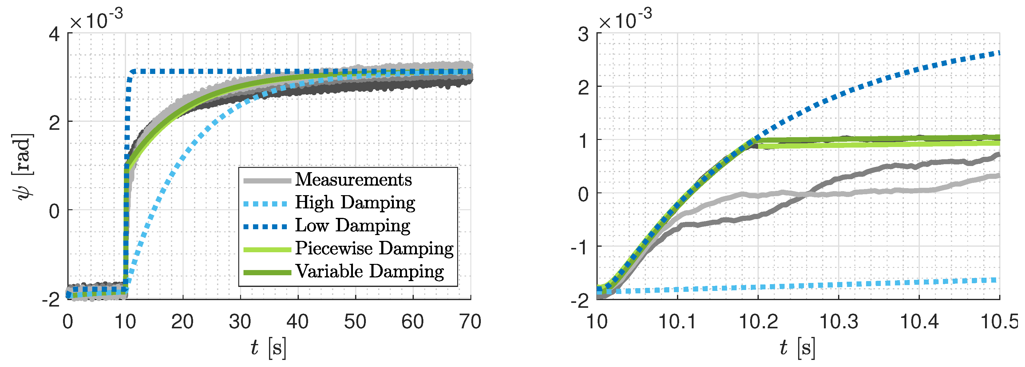
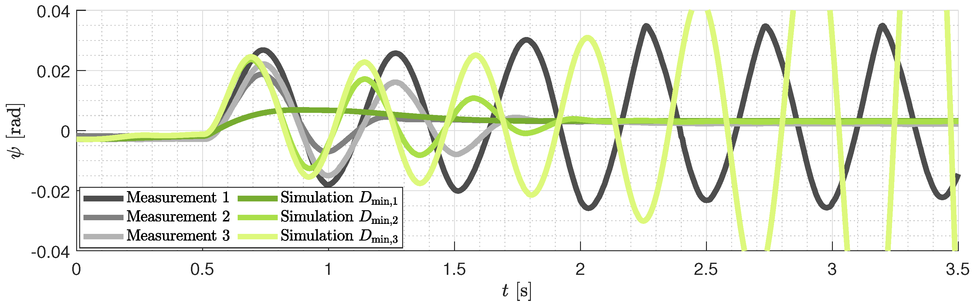
4.3.3. Damping Modeling and Identification

Naturally, by restoring the contact between wheels and roller, the damping behavior changes compared to the previous section and only the numerical value of parameter ${\omega }_0$ can be used for the model. Further, as discussed in Section 3, damping D appears to be not constant but varying over the course of a step response. Thus, measurements were carried out that allowed for a longer time period after the step occurred. Three of these measurements can be seen in Figure 8 in three different shades of grey. It can be observed that these step responses can be divided into one part before around 0.2 s with very small damping and the reaming part where the damping is very high. This can be quantified by splitting the step response and carrying out optimization problem (1) for $t_{\mathrm{start}}=10$, $t_{\mathrm{end}}=10.2$ and $t_{\mathrm{start}}=10.2$, $t_{\mathrm{end}}=70$. Parameters K, ${\psi }_{\mathrm{off}}$ are easily obtained from the stationary values of the step response, allowing to neglect the hysteresis, i.e., $f_{\mathrm{hyst}}(\dot{\psi },z)=0$ leaving only the damping parameter $c=D$ for optimization. The parameters including the resulting damping values can be found in Table 3. It can be seen that even the lower damping value corresponds to an overdamped system. In Figure 8, it can be seen that the light green step response resulting from these piecewisely defined two dampings leads to a response that aligns very well with the measurement used to fit, especially when compared to the variance of the three step responses. It can also be seen that the two step responses in light and dark blue with the corresponding constant low and high damping values from Table 3 over the whole time period lead to large errors and do not capture the desired system behavior. The key question remaining is how can the change in damping be modeled accordingly and what are the variables and states the change depends on. Different experiments have shown that quick changes in the input lead to smaller damping, which motivates modeling the damping as a function of the derivative of the velocity. Furthermore, in order to keep the damping within bounds, it is convenient to introduce a saturation as well, i.e., the damping is obtained in a piecewise linear manner as

$$\begin{array}{c}\hfill D\left(\dot{u}\right)=\left\{\begin{array}{cc}{D}_{\min }\hfill & |\dot{u}|>=c_{{\dot{u}}_{\max }}\hfill \\ -{\displaystyle \frac{|\dot{u}|}{c_{{\dot{u}}_{\max }}}}(D_{\max }-D_{\min })+D_{\max }\hfill & |\dot{u}|<c_{{\dot{u}}_{\max }}\hfill \end{array}\right..\end{array}$$

(7)

As the input function is not necessarily differentiable, the derivative of the input is obtained from the low-pass filtered input signal with an edge frequency of 10 Hz. With these adjustments, optimization (1) is carried out with the variable damping (7) with $D_{\min }$, $D_{\max }$ as the results of the previous optimization results and $c=c_{{\dot{u}}_{\max }}$ as the only tuning variable and $t_{\mathrm{start}}=0$, $t_{\mathrm{end}}=80$. The parameter can be found in Table 3 and the simulation result in Figure 8. It can be seen that the response aligns closely with the piecewise damping response and therefore also with the measurements.

4.3.4. Hysteresis Modeling and Identification

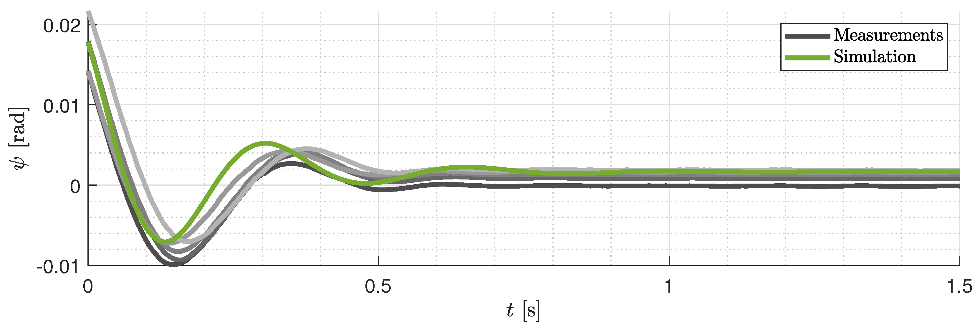
It remains to model the hysteresis, which plays a significant role particularly in the steady state values as can be seen in Section 3. Hysteresis is widely understood as a nonlinear phenomenon due to which a dynamic system does not provide the same input–ouput relation for low-frequency inputs when loading or unloading [31]. Or, in different words, for a linear system in the form of (6) with $f_{\mathrm{hyst}}(\dot{\psi },z)=0$ and a sinusoidal input $\Delta u=sin\left(2\pi \nu t\right)$, the plot of $\psi$ over $\Delta u$ is an ellipse which semi-minor axis vanishes for decreasing $\nu$ and converges to a simple line described by $\psi =K\Delta u+{\psi }_{\mathrm{off}}$ for $\nu \to 0$. However, if the semi-minor axis of the ellipse does not vanish and is independent of the frequency, this is referred to as a ”rated-independent hysteresis” [32]. This behavior is illustrated in Figure 9, where the linear system is simulated for the higher damping obtained in the previous section and the input $\Delta u=Asin\left(2\pi {\nu }_{i}t\right)$ with $i\in \{1,2\}$, where ${\nu }_1=4.8$ mHz, and even lower frequency ${\nu }_2=2.4$ mHz. It can be observed that the minor axis of the dark orange ellipse, representing the higher frequency ${\nu }_1$, decreases in size compared to the lighter orange ellipse, which represents the smaller frequency ${\nu }_2$. In contrast, the results of the measurements displayed in light and dark grey show only minor changes between the two different frequencies. In order to capture this behavior, a hysteresis term is introduced. This can be achieved in different ways as there exist multiple approaches to model hysteresis, e.g., the Preisach model [33], the Duhem model [34], or the Prandtl–Ishlinskii model [35] to name but a few. In this work, we decided to use the Bouc Wen model [31] due to its compactness and manageable number of variables. This model defines the term

$$\begin{array}{c}\hfill f_{\mathrm{hyst}}(\dot{\psi },z)={\omega }_0^2\psi -{\omega }_0^2(a_{\mathrm{Bouc}}\psi +(1-a_{\mathrm{Bouc}})z_{\mathrm{Hyst}})\end{array}$$

(8)

where parameter $a_{\mathrm{Bouc}}\in [0,1]$ represents the ratio of the back-to-front stiffness of the yield value, i.e., when $a_{\mathrm{Bouc}}=1$, the system has an ordinary linear elasticity as $f_{\mathrm{hyst}}(\dot{\psi },z_{\mathrm{hyst}})=0$. State $z_{\mathrm{hyst}}$ is defined by the differential equation

$$\begin{array}{c}\hfill {\dot{z}}_{\mathrm{hyst}}=A_{\mathrm{Bouc}}\dot{\psi }-{\beta }_{\mathrm{Bouc}}|\dot{\psi }\left|\right|z_{\mathrm{hyst}}{|}^{n_{\mathrm{Bouc}}-1}{z}_{\mathrm{hyst}}-{\gamma }_{\mathrm{Bouc}}\dot{\psi }{\left|z_{\mathrm{hyst}}\right|}^{n_{\mathrm{Bouc}}}\end{array}$$

(9)

where $A_{\mathrm{Bouc}}\in \mathbb{R}$, ${\beta }_{\mathrm{Bouc}}>0$, ${\gamma }_{\mathrm{Bouc}}\in \mathbb{R}$ and $n_{\mathrm{Bouc}}\in \mathbb{N}$ are dimensionless parameters controlling the behavior of the model. These parameters are not straightforward to interpret, and efforts to address this limitation through identification and investigation were made [36]. The set of parameters was shown to be redundant [37]; thus, parameter $A_{\mathrm{Bouc}}$ was set to 1. Additionally, parameter $n_{\mathrm{Bouc}}$ was chosen to be 1 to reduce the complexity of the model.

Parameter K was easily obtained solving optimization problem (1) for the linear system with $f_{\mathrm{hyst}}(\dot{\psi },z)=0$, where there are parameters D and ${\omega }_0$ from the previous fits or the simple consideration of approximating the ellipse of Figure 9 by a line with ${\displaystyle \frac{\psi }{\Delta u}}\approx {\displaystyle \frac{-0.006-0.003}{-0.7-0.7}}=0.0064$. The optimization result is found in Table 3. The remaining parameters $c=[{\psi }_{\mathrm{off}},a_{\mathrm{Bouc}},{\beta }_{\mathrm{Bouc}},{\gamma }_{\mathrm{Bouc}}]$ were obtained solving optimization problem (1) with the previously identified parameter $K,{\omega }_0$ and higher damping D. The optimization results can be found in Table 3 and the resulting simulation trajectory can be seen in Figure 9 for frequency ${\nu }_1$ and ${\nu }_2$ displayed in green. It can be seen that the results match the measured trajectories closely and are barely influenced by the change in frequency as desired.

4.3.5. Verification

In order to verify the results of the modeling and identification of the previous section, an independent measurement is used. The measurement introduced in the motivation is not used for the parameter fit and is therefore used for the verification as it showcases both the influence of the variable damping and the hysteresis. For the simulation, model (6), (9) with (8), variable damping model (7), and the optimized parameters of Table 3 from the last row and $c_{{\dot{u}}_{\max }}$ of the second to last row are used. In Figure 10, the simulation results are shown with three measurements. It can be observed that the simulation follows the measurements for the application purpose in a sufficient manner. The measured steps exhibit two different damping behaviors, a characteristic that is also apparent in the simulation. While the dynamics of the first step align well, subsequent steps show some offsets. However, towards the final steps, the simulations once again closely match the measurements.

This indicates that the proposed model effectively captures the hysteresis effect, though it does not precisely replicate the induced offsets. Nevertheless, this level of fidelity is adequate as it models the primary effects to be addressed by a controller. Overall, the model with the identified parameters accurately represents the system behavior and represents a significant improvement over the academic models and parameters used in previous studies. Particularly noteworthy are the representations of variable damping and hysteresis, crucial considerations for the controller design discussed in the subsequent section.

5. Closed-Loop System and Control Design

In this section, we undertake control design based on the model and parameters developed in the previous section. Although nonlinear effects like hysteresis and variable damping imply a need for advanced control strategies such as feedforward control or robust methods like sliding mode control, this study concentrates on proposing straightforward controllers with minimal complexity. These controllers facilitate quick adaptation to environmental changes while effectively mitigating major drawbacks associated with these effects, such as steady-state error and destabilization. The design of more sophisticated control architectures is left for future research. For the design of the control and stability proof, the linear part of system (6) combined with lateral dynamics (2b) is used. This can be formulated in state space as $\dot{x}=Ax+Bu$, where $x={\left[\begin{array}{ccc}y& \psi & \dot{\psi }\end{array}\right]}^{\top }+A^{-1}{x}_{\mathrm{off}}$ with $x_{\mathrm{off}}={\left[\begin{array}{ccc}{\displaystyle \frac{{\overline{c}}_y}{2l_0}}v(y_{\mathrm{f}}+y_{\mathrm{off}})& 0& w_0^2{\psi }_{\mathrm{off}}\end{array}\right]}^{\top }$ and

$$\begin{array}{ccc}\hfill A=\left[\begin{array}{ccc}-{\displaystyle \frac{v{\overline{c}}_y}{2l_0}}& v{\overline{c}}_y& 0\\ 0& 0& 1\\ 0& -{\omega }_0^2& -2D{\omega }_0\end{array}\right]& \hfill & \hfill B=\left[\begin{array}{c}0\\ 0\\ K{\omega }_0^2\end{array}\right].\end{array}$$

(10)

Two control designs are discussed in this section. First, a simple P-control law is introduced to demonstrate the fundamental principles of system control while also highlighting the limitations of such a basic approach. Following this, a cascaded PI-PD control scheme is proposed. This design offers sufficient flexibility to meet closed-loop requirements effectively while also enabling straightforward gain tuning strategies.

5.1. P Control Design

As discussed in Section 4.1, the rear wheel carrier lateral dynamics are stable. Combined with the yaw dynamics of system (10), this also leads to an open-loop stable system. Therefore, the control of the rear wheel carrier mainly robustifies the system and improves its dynamics. Keeping in mind that $l_0$ is large for a 1:1 prototype, it should be noted that system (10) contains a pole at 0 for $l_0\to \infty$. This makes a control indispensable to obtain a stable system. In this case, due to the form of the system, however, a P-controller is sufficient to stabilize the system. Thus, such a P-control is investigated in this system to establish a baseline performance and also validate the model proposed in the previous sections on the closed-loop system. Figure 11 shows the root locus of system (10) for output y and input $u=K_{\mathrm{P}}(y_{\mathrm{ref}}-y)$. The crosses indicate the three poles for the open-loop system. It can be seen that due to the yaw dynamics being overdamped, one of the poles is very far in the left half plane while the other two have a real part of $-4.5$ and $-1.73$. The latter two eigenvalues bifurcate into a complex pole pair for rising $K_{\mathrm{P}}$ and reach the right half plane for $K_{\mathrm{P}}>18605$, indicating that the choice of $K_{\mathrm{P}}$ must be taken with care as it might lead to an unstable system. Naturally, this stability boundary depends on the damping of the yaw dynamics, and as discussed in Section 4.3.3, this damping varies dependent on the input and is not easy to model. With this in mind, the evolution of the poles with the highest real value is shown in Figure 12 for different damping D. It can be observed that an optimal gain $K_{\mathrm{P}}$ exists for every D, which leads to the lowest possible real part. If the gain is higher than the optimal value, the real part rises until the system becomes unstable, while for smaller values, the real part is smaller, and therefore not the best possible performance is reached. For high damping, a similar behavior can be observed. For very high damping, the optimal $K_{\mathrm{P}}$ value is also very high, and the stability boundary is also consequently much higher.

These considerations together with the previous identification of the damping suggest that the choice of $K_{\mathrm{p}}=500$ is close to the optimum while also offering enough margin to the instability boundary. The yaw angle $\psi$ of the closed-loop system for this control can be seen in Figure 13, where a step of $\Delta y=0.2$ mm is followed. The three different measurements for the same setup can be seen in the three different shades of grey while three measurements for $D\in \{0.04,0.06,2\}$ are displayed. It can be observed that the three measurements behave very differently despite these measurements being from the same setup. Two of the measurements converge to a constant value with different dampings, while the first measurement indicates that the system is unstable. This behavior shows that there is also a dynamic in the system that is not modeled in the proposed system. However, it can be seen that adjusting the damping value leads to an unstable response as well. Notably, this damping value is around 100 times smaller than the one identified in Section 4.3.3 due to the high frequent input. Combined with the fact that the closed loop with the proposed control law does not admit a consistent system behavior, this renders a simple P controller insufficient for the real test rig. Thus, a different control is proposed that generates consistent system behavior.

5.2. Cascaded PI-PD Control

In this section, we propose the usage of a cascaded PI-PD control design illustrated in Figure 14. The section is divided into four parts. First, the structure of the control is presented, as well as the resulting closed-loop dynamics. Second, methods and guidelines for the gain tuning are proposed. Third, the performance of the proposed controller is assessed on the test rig by observing its response to a sequence of step inputs while simultaneously verifying the model presented in Section 4. Finally, the robustness of the control is investigated by applying various perturbations to the test rig.

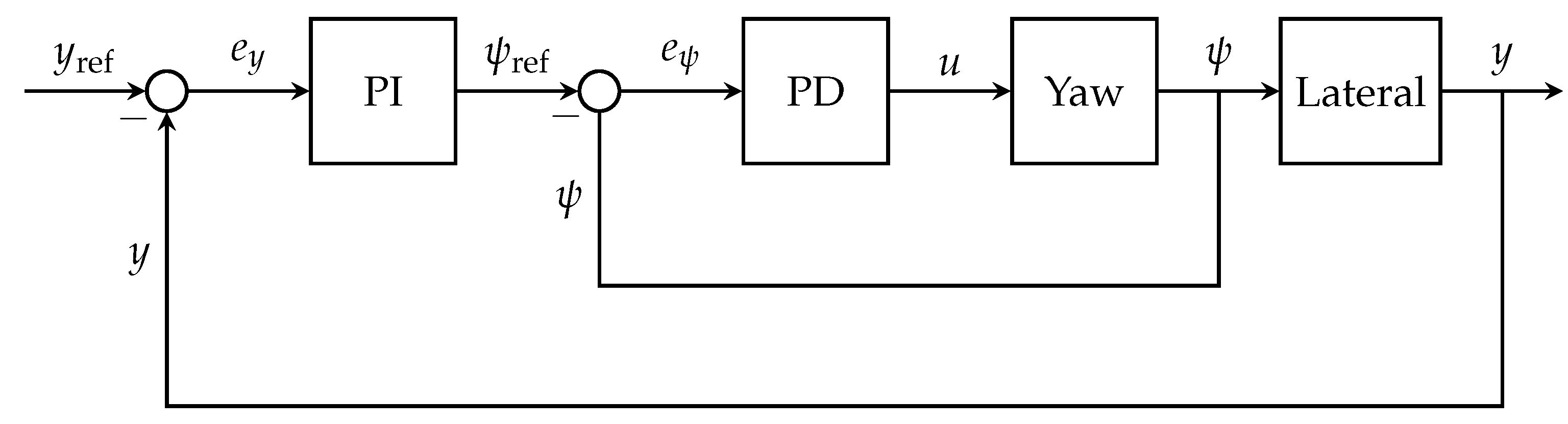
5.2.1. Control Structure

The previous observations have shown that there are multiple key points that must be taken into account when designing the control law. First, the damping of the system is not constant and it is therefore advisable to add damping by the means of control to obtain a robustly stable system. Second, the change in damping and the inconsistency of the system occurs mainly for large and high frequent input u. Thus, the control parameters should be chosen such that a maximal threshold is not exceeded.

Due to the staircase form of system (10) and the points mentioned beforehand, the design of a cascaded control is proposed. Its structure is illustrated in Figure 14 with an inner PD control defined for a reference yaw angle ${\psi }_{\mathrm{ref}}$,

$$\begin{array}{c}\hfill u=K_{\mathrm{P},\psi }{e}_{\psi }+K_{\mathrm{D},\psi }{\widehat{e}}_{\dot{\psi }}\end{array}$$

(11)

with tuning parameters $K_{\mathrm{P},\psi },K_{\mathrm{D},\psi }\in \mathbb{R}$, where $e_{\psi }={\psi }_{\mathrm{ref}}-\psi$ and ${\widehat{e}}_{\dot{\psi }}$ is an estimation of the derivative of the error $e_{\dot{\psi }}={\dot{\psi }}_{\mathrm{ref}}-\dot{\psi }$ provided by a standard linear differentiator with transfer function $G\left(s\right)={\displaystyle \frac{s}{T_{\mathrm{f}}s+1}}$ defined in state space by ${\widehat{e}}_{\dot{\psi }}={\dot{\psi }}_{\mathrm{ref}}-\widehat{\dot{\psi }}$ where

$$\begin{array}{cccc}\hfill {\dot{x}}_{\mathrm{diff}}& =-{\displaystyle \frac{1}{T_{\mathrm{f},\psi }}}{x}_{\mathrm{diff}}+\psi ,\hfill & \hfill \widehat{\dot{\psi }}& =-{\displaystyle \frac{1}{T_{\mathrm{f},\psi }^2}}{x}_{\mathrm{diff}}+{\displaystyle \frac{1}{T_{\mathrm{f},\psi }}}\psi \hfill \end{array}$$

(12)

with the tuning parameter $T_{f,\psi }\in \mathbb{R}$ close to zero. The reference yaw angle is given by the outer PI controller,

$$\begin{array}{c}\hfill {\psi }_{\mathrm{ref}}=K_{\mathrm{P},y}{e}_y+K_{\mathrm{I},y}{x}_{\mathrm{I}}\end{array}$$

(13)

where $K_{\mathrm{P},y},K_{\mathrm{I},y}\in \mathbb{R}$ are the tuning parameters, $e_y=y_{\mathrm{ref}}-y$ is the displacement error, and $x_{\mathrm{I}}$ is this error integrated over time, i.e.,

$$\begin{array}{c}\hfill {\dot{x}}_{\mathrm{I}}\left(t\right)=e_y.\end{array}$$

(14)

5.2.2. Closed-Loop Dynamics

The closed inner loop is obtained combining the yaw dynamics (10) and control (11). In the ideal case, if $\dot{\psi }$ is available and is not approximated by (12), the closed loop is defined by ${\dot{e}}_{\psi ,\dot{\psi }}=A_{\psi ,\mathrm{cl}}{e}_{\psi ,\dot{\psi }}+g_{\psi ,\dot{\psi }}({\psi }_{\mathrm{ref}},{\dot{\psi }}_{\mathrm{ref}},{\ddot{\psi }}_{\mathrm{ref}})$ with $e_{\psi ,\dot{\psi }}={[{\psi }_{\mathrm{ref}}-(\psi -{\psi }_{\mathrm{off}}){\dot{\psi }}_{\mathrm{ref}}-\dot{\psi }]}^{\top }$ and

$$\begin{array}{ccc}\hfill A_{\psi ,\mathrm{cl}}=A_{\psi }-B_{\psi }\left[\begin{array}{cc}{K}_{\mathrm{P}}& K_{\mathrm{D}}\end{array}\right]& \hfill & \hfill g_{\psi ,\dot{\psi }}({\psi }_{\mathrm{ref}},{\dot{\psi }}_{\mathrm{ref}},{\ddot{\psi }}_{\mathrm{ref}})=\left[\begin{array}{c}{\dot{\psi }}_{\mathrm{ref}}\\ {\ddot{\psi }}_{\mathrm{ref}}\end{array}\right]-A_{\psi }\left[\begin{array}{c}{\psi }_{\mathrm{ref}}\\ {\dot{\psi }}_{\mathrm{ref}}\end{array}\right]\end{array}$$

(15)

where $A_{\psi }=A_{2:3,2:3}$ and $B_{\psi }=B_{2:3}$ denote the submatrices of the dynamics matrices in Equation (10) governing the yaw dynamics. If $\dot{\psi }$ is not available and the approximation $\widehat{\dot{\psi }}$ defined by (12) based on $\psi$ is carried out, the closed loop is of one dimension higher. It has the form ${\dot{\overline{e}}}_{\psi ,\dot{\psi }}={\overline{A}}_{\psi ,\mathrm{cl}}{\overline{e}}_{\psi ,\dot{\psi }}+{\overline{g}}_{\psi ,\dot{\psi }}\left(t\right)$ with ${\overline{e}}_{\psi ,\dot{\psi }}={\left[e_{\psi ,\dot{\psi }}{x}_{\mathrm{diff}}\right]}^{\top }$ and

$$\begin{array}{ccc}\hfill {\overline{A}}_{\psi ,\mathrm{cl}}& =\left[\begin{array}{ccc}0& 1& 0\\ -{\omega }_0^2-K{\omega }_0^2(K_p+{\displaystyle \frac{K_{\mathrm{D}}}{T_{\mathrm{f},\psi }}})& -2D{\omega }_0& -{\displaystyle \frac{K{K}_{\mathrm{D}}{\omega }_0^2}{T^2}}\\ -1& 0& -{\displaystyle \frac{1}{T_{\mathrm{f},\psi }}}\end{array}\right]\hfill & \hfill \end{array}$$

(16a)

$$\begin{array}{cc}\hfill g_{\psi ,\dot{\psi }}({\psi }_{\mathrm{ref}},{\dot{\psi }}_{\mathrm{ref}},{\ddot{\psi }}_{\mathrm{ref}})& =\left[\begin{array}{c}0\\ {\ddot{\psi }}_{\mathrm{ref}}+{\psi }_{\mathrm{ref}}{\omega }_0^2+{\displaystyle \frac{K}{T}}{K}_{d,\psi }{\psi }_{\mathrm{ref}}{\omega }_0^2+2D{\dot{\psi }}_{\mathrm{ref}}{\omega }_0-K{K}_{d,\psi }{\dot{\psi }}_{\mathrm{ref}}{\omega }_0^2\\ {\psi }_{\mathrm{ref}}\end{array}\right].\hfill \end{array}$$

(16b)

Naturally, the eigenvalues of ${\overline{A}}_{\psi ,\mathrm{cl}}$ converge to the eigenvalues of $A_{\psi ,\mathrm{cl}}$ for $T_{\mathrm{f},\psi }$ converging to zero.

Considering the outer loop and assuming that the inner loop is very fast such that the assumption $\psi ={\psi }_{\mathrm{ref}}$ holds, where ${\psi }_{\mathrm{ref}}$ is defined in (13), the following system is obtained:

$$\begin{array}{ccc}\hfill A_{y,x_{\mathrm{I}}}=\left[\begin{array}{cc}0& 1\\ K_{\mathrm{I},y}{\overline{c}}_{y}v& -{\displaystyle \frac{{\overline{c}}_{y}v}{l_0}}-{\overline{c}}_{y}v{K}_{\mathrm{P},y}\end{array}\right]& \hfill & \hfill g_{y,x_{\mathrm{I}}}=\left[\begin{array}{c}0\\ {\displaystyle \frac{{\overline{c}}_{y}v}{l_0}}{y}_{\mathrm{ref}}+l_0{\dot{y}}_{\mathrm{ref}}\end{array}\right].\end{array}$$

(17)

In order to define the closed outer loop without this assumption, more extensive calculations have to be carried out. In order to achieve this, we use $e_{1}AB=0$ and obtain, iteratively, relations

$$\begin{array}{cc}\hspace{1em}\hspace{1em}\hspace{1em}\dot{y}=e_1(Ax+Bu)\hfill & \hspace{1em}\hspace{1em}\hspace{1em}\ddot{y}=e_1(A^{2}x+Bu)\hfill \end{array}$$

(18a)

$$\begin{array}{cc}\hfill {\dot{e}}_y={\dot{y}}_{\mathrm{ref}}-\dot{y}\hspace{1em}\hspace{1em}\hspace{1em}\hspace{1em}\hspace{1em}\hfill & {\ddot{e}}_y={\ddot{y}}_{\mathrm{ref}}-\ddot{y}\hfill \end{array}$$

(18b)

$$\begin{array}{cc}\hspace{1em}\hspace{1em}{\dot{\psi }}_{\mathrm{ref}}=K_{\mathrm{P},y}{\dot{e}}_y+K_{\mathrm{I},y}{e}_y\hfill & \hspace{1em}\hspace{1em}{\ddot{\psi }}_{\mathrm{ref}}=K_{\mathrm{P},y}{\ddot{e}}_y+K_{\mathrm{I},y}{\dot{e}}_y.\hfill \end{array}$$

(18c)

Using Equation (14), (18b) and substituting the variables from Equation (18) into Equation (15) allows to define the complete dynamics as $f\left(e\right)=\left[{\dot{x}}_{\mathrm{I}}{\dot{e}}_y{\dot{e}}_{\psi ,\dot{\psi }}\right]$. These dynamics may be written in linear fashion as $\dot{e}=A_{\mathrm{cl}}e+g(y_{\mathrm{ref}},{\dot{y}}_{\mathrm{ref}},{\ddot{y}}_{\mathrm{ref}})$ with $e={\left[x_{\mathrm{I}}{e}_y{e}_{\psi ,\dot{\psi }}\right]}^{\top }$ and

$$\begin{array}{ccc}\hfill A_{\mathrm{cl}}={\displaystyle \frac{\partial f\left(e\right)}{\partial e}}& \hfill & \hfill g(y_{\mathrm{ref}},{\dot{y}}_{\mathrm{ref}},{\ddot{y}}_{\mathrm{ref}})=f\left(e\right)-A_{\mathrm{cl}}e.\end{array}$$

(19)

Note that g is not a function of e any more but only of the lateral reference vector and its derivatives due to the linearity of the individual components in $f\left(e\right)$. This derivation has shown how to obtain the system for $\dot{\psi }$ available, e.g., by means of measurements. The analogue derivation using ${\overline{e}}_{\psi ,\dot{\psi }}$ and Equation (16) instead of $e_{\psi ,\dot{\psi }}$ and (15) leads to variables $\overline{e}$, ${\overline{A}}_{\mathrm{cl}}$ and $g_{\mathrm{cl}}$ if $\dot{\psi }$ is obtained by means of numerical differentiation.

5.2.3. Gain Tuning

Selecting the gains $K_{\mathrm{P},y}$, $K_{\mathrm{I},y}$, $K_{\mathrm{P},\psi }$, $K_{\mathrm{D},\dot{\psi }}$, $T_{\mathrm{f},\psi }$ is crucial for ensuring effective control performance and robustness. A procedure on tuning these parameters is presented to ensure that (i) the constraints in Table 2 are satisfied in the case of maximum tracking error, (ii) stability can be guaranteed, and iii) finding a good performance/robustness tradeoff by placing the inner and outer loop poles accordingly.

Numerous methods exist for tuning these parameters, yet the task is not trivial. While the proposed control resembles full-state feedback, typically achieved through pole placement, its cascaded structure simplifies design and allows iterative parameter adjustments. This facilitates quick adaptation to varying system conditions during field tests. A procedure on tuning these parameters is presented in the following. The resulting gains are presented in

Table 4. Tuned parameters.

Inner Loop Parameter	Value	Outer Loop Parameter	Value
$K_{\mathrm{P},\psi }$	40	$K_{\mathrm{P},y}$	3
$K_{\mathrm{D},\psi }$	5	$K_{\mathrm{I},x_{\mathrm{I}}}$	9
$T_{\mathrm{f},\psi }$	0.3

.

The first step involves tuning the inner loop using $K_{\mathrm{P},\psi }$, $K_{\mathrm{D},\psi }$, and Equation (15). As seen in Section 4.3.3 and Section 5.1, the damping parameter may vary heavily with the inputs of high dynamics. Therefore, $K_{\mathrm{D},\psi }$ should be sufficiently high to ensure damping and compensate for uncertain parameters while avoiding amplification of measurement noise beyond the system’s stability limits. On the flipside, parameters $K_{\mathrm{P},\psi }$, $K_{\mathrm{D},\psi }$ should be chosen small enough to keep the input small to reduce the uncertainty of D and induce a better robustness. Based on the previous sections and measurements, the developed criterion is chosen such that for a maximal yaw angle $0.05\mathrm{rad}$ as given in Table 2 and rate $0.4$ rad s⁻¹, the resulting input should not exceed 2 A. This leads to gains $K_{\mathrm{P},\psi }=40$, $K_{\mathrm{D},\psi }=5$ yielding eigenvalues of $[-88.9,-5.0]$ for closed-loop matrix (15).

In the second step, $T_{\mathrm{f},\psi }$ is selected such that the measurement noise is not too heavily amplified and the eigenvalues of (16) are in a similar region as the ones from (15). Choosing $T_{\mathrm{f},\psi }=0.3$ leads to eigenvalues $[-67.1,-40.7,-4.9]$, so in particular, the slowest eigenvalue is of the same magnitude as in the ideal case, which deems the choice of $T_{\mathrm{f},\psi }$ suitable.

As the third step, parameters $K_{\mathrm{P},y}$, $K_{\mathrm{I},y}$ of the outer loop are designed using the dynamics presented in Equation (17). It can be easily seen that already small control gains lead to a stable system with sufficiently fast eigenvalues. However, a choice of sufficiently high $K_{\mathrm{I},y}$ is important as this is currently the only part of the control counteracting the stationary influence of the hysteresis. In a similar manner as before, we formulate as a task that for a maximal lateral displacement of $0.008$ mm the desired yaw angle is smaller than $0.06\mathrm{rad}$ and that the slowest eigenvalue is not smaller than $-1.5$. This leads to parameters $K_{\mathrm{P},y}=3$ and $K_{\mathrm{I},x_{\mathrm{I}}}=9$ which leads to eigenvalues $[-4.5,-2.0]$.

As the final step, the eigenvalues of the complete closed-loop system (19) are verified to ensure they remain in a similar range as those designed for the inner and outer loops. In the proposed case, the resulting eigenvalues $[-66.5,-41.0,-4.4,-3.7,-0.5]$ are mostly within the expected range, with the slowest eigenvalues slightly slower than initially designed. This discrepancy does not compromise the satisfactory dynamics and robustness demonstrated in the following sections.

5.2.4. Performance

In this section, the performance of the proposed controller with the gains developed in Section 5.2.3 is investigated by applying the control for lateral reference signal similar to the one in Section 3. The reference signal consists of a sequence of steps from 0 to $y_{\mathrm{final}}$ where $y_{\mathrm{final}}\in \{-3.5,-3.3,\dots 3.5\}$. This reference signal showcases the stationary convergence of the closed-loop system despite the significant influence of the hysteresis while also showcasing the dynamics properties. Additionally, the simulation with the model developed in Section 4.1, Section 4.2 and Section 4.3 and the parameters from Table 1 are discussed. The lateral displacement, yaw angle, differential angular velocity, and input can be seen in Figure 15 and Figure 16. Both plots show three different measurements of the same scenario in different shades of grey, and the simulations results aremin green. First, we point out that the three measurements align very closely, showing that the closed loop under this control yields very consistent results, especially when compared to the measurements in Section 5.1 where even the stability properties vary. For the simulation results, it can be seen that the simulated lateral displacement, yaw angle, angular velocity, and input align very well with the real measured lateral displacements. For the performance of the control, it can be seen that input u is well within the saturation limits of 4 A given in Table 2. Additionally, the reference is followed closely with a rising time of around 2.7 s, a small overshoot of $6\%$, and a $2\%$ settling time of around 7.3 s. All in all, the proposed control offers satisfying and consistent results, fast transitional behavior, and negligible steady–state error.

5.2.5. Robustness

The robustness of the controller with the gains developed in Section 5.2.3 is examined in this section. To evaluate this, the reference lateral displacement is set to a constant zero, and disturbances are applied to the system. Specifically, at 10 $\mathrm{s}$, 15 $\mathrm{s}$, and 20 $\mathrm{s}$, rapid perturbations with increasing amplitudes simulate the effects of rail irregularities. At 25 $\mathrm{s}$ and 45 $\mathrm{s}$, an approximately constant force is applied to the test rig for 10 $\mathrm{s}$, mimicking the effect of side wind. The measured force and torque of the right force–torque sensor are shown in Figure 17, while the measured lateral displacement is depicted in Figure 18.

It is observed that during the initial three rapid perturbations, the lateral displacement changes significantly within a few seconds but returns to the desired value within approximately 3 $\mathrm{s}$. Naturally, higher perturbation forces lead to larger induced lateral displacements, though they still converge back to the desired steady state.

For the constant force perturbations, an initial lateral displacement is induced, but the integrator part of the controller generates a corrective force that brings the lateral displacement back to zero. Upon removal of the perturbation, new transient behavior occurs as the integrator adjusts to the absence of the disturbance.

Overall, the proposed controller design exhibits robust behavior. The system is resistant to destabilization by high-magnitude perturbations, and constant-magnitude disturbances can be effectively compensated by the controller.

5.2.6. Discussion

Overall, the proposed cascaded PI-PD controller demonstrates satisfactory performance. The lateral displacement tracks its reference quickly, with minimal overshoot. The integral component of the controller effectively compensates for the steady-state effects of hysteresis. The closed-loop system also exhibits robustness against both constant and rapid disturbances, all achieved with a simple control structure and easily tunable gains.

However, this straightforward design has its limitations in terms of performance and adaptability to varying working conditions. A more tailored control design, specifically addressing the variable damping phenomenon, could further enhance tracking performance and ensure system stability. The same applies to adapting the controller to different operational conditions.

Future work should explore whether a single set of gains can provide robust and high-performance control under all operating conditions, including high side-slip scenarios, or if some form of online gain adaptation is required to achieve optimal results.

6. Conclusions

In this work, we successfully adapted theoretical models to practical applications for the lateral control of independently rotating driven wheels (IRDWs) using a 1:5 scaled test rig developed by DLR. The parameter identification process proved effective, yielding small errors that validate the accuracy of the derived model. However, challenges remain, particularly in accurately modeling yaw dynamics, variable damping, and hysteresis behavior, all of which are critical factors influencing the system’s overall dynamics.

The designed PI-PD controller demonstrates good performance, with rise and settling times on the order of a few seconds, indicating a rapid and stable response. Furthermore, the controller shows robustness against both constant forces and short, strong disturbances, ensuring reliable operation under controlled conditions. Despite these promising results, it is important to recognize that the current conclusions are based on laboratory conditions. Real-world applications, where safety is paramount, introduce additional complexities. For example, IRDWs are particularly susceptible in cases of motor outages, as lateral stability is no longer passively maintained. Future work will focus on reconfiguration scenarios to mitigate these risks and ensure a safer, more reliable system in the event of component failures.

Regarding efficiency, IRDWs offer potential advantages by allowing precise tracking of lateral displacement, which can reduce wheel wear. This could lead to less frequent replacement of wheels, lowering maintenance costs, and enhancing the system’s long-term efficiency. However, further investigations are needed to quantify these efficiency gains under real operating conditions, particularly considering variations in track and weather environments.

In summary, while the PI-PD controller shows promise in improving the lateral stability and performance of IRDWs, further work is necessary to fully validate its robustness, safety, and efficiency in broader operational contexts. This ongoing research will contribute to advancing railway vehicle technology with improved safety, reliability, and reduced maintenance requirements.

References

1. Suda, Y.; Michitsuji, Y. Improved curving performance using unconventional wheelset guidance design and wheel-rail interface–Present and future solutions. Veh. Syst. Dyn. 2023, 61, 1881–1915. [Google Scholar] [CrossRef]
2. Kurzeck, B.; Valente, L. A novel mechatronic running gear: Concept, simulation and scaled roller rig testing. In Proceedings of the World Congress on Railway Research, Mai 2011, Lille, France, 22–26 May 2011. [Google Scholar]
3. Jaschinski, A. On the Application of Similarity Laws to a Scaled Railway Bogie Model. 1991. Available online: https://elibrary.ru/item.asp?id=6848485 (accessed on 3 October 2024).
4. Kurzeck, B.; Heckmann, A.; Wesseler, C.; Rapp, M. Mechatronic track guidance on disturbed track: The trade-off between actuator performance and wheel wear. Veh. Syst. Dyn. 2014, 52, 109–124. [Google Scholar] [CrossRef]
5. Keck, A.; Schwarz, C.; Meurer, T.; Heckmann, A.; Grether, G. Estimating the wheel lateral position of a mechatronic railway running gear with nonlinear wheel–rail geometry. Mechatronics 2020, 73, 102457. [Google Scholar] [CrossRef]
6. Myamlin, S.; Kalivoda, J.; Neduzha, L. Testing of railway vehicles using roller rigs. Procedia Eng. 2017, 187, 688–695. [Google Scholar] [CrossRef]
7. Kalivoda, J.; Bauer, P. Scaled roller rig to assess the influence of active wheelset steering on wheel-rail contact forces. In Proceedings of the IAVSD International Symposium on Dynamics of Vehicles on Roads and Tracks, Gothenburg, Sweden, 12–16 August 2019; pp. 82–89. [Google Scholar]
8. Oh, Y.J.; Lee, J.K.; Liu, H.C.; Cho, S.; Lee, J.; Lee, H.J. Hardware-in-the-loop simulation for active control of tramcars with independently rotating wheels. IEEE Access 2019, 7, 71252–71261. [Google Scholar] [CrossRef]
9. Jia, X.; Yin, Y.; Wang, W. Dynamic Modeling, Dynamic Characteristics, and Slight Self-Guidance Ability at High Speeds of Independently Rotating Wheelset for Railway Vehicles. Appl. Sci. 2024, 14, 1548. [Google Scholar] [CrossRef]
10. Suda, Y.; Wang, W.; Nishina, M.; Lin, S.; Michitsuji, Y. Self-steering ability of the proposed new concept of independently rotating wheels using inverse tread conicity. Veh. Syst. Dyn. 2012, 50, 291–302. [Google Scholar] [CrossRef]
11. Ji, Y.; Ren, L.; Zhou, J. Boundary conditions of active steering control of independent rotating wheelset based on hub motor and wheel rotating speed difference feedback. Veh. Syst. Dyn. 2018, 56, 1883–1898. [Google Scholar] [CrossRef]
12. Perez, J.; Busturia, J.M.; Mei, T.; Vinolas, J. Combined active steering and traction for mechatronic bogie vehicles with independently rotating wheels. Annu. Rev. Control 2004, 28, 207–217. [Google Scholar] [CrossRef]
13. Liu, X.; Goodall, R.; Iwnicki, S. Active control of independently-rotating wheels with gyroscopes and tachometers–simple solutions for perfect curving and high stability performance. Veh. Syst. Dyn. 2021, 59, 1719–1734. [Google Scholar] [CrossRef]
14. Ahn, H.; Lee, H.; Go, S.; Cho, Y.; Lee, J. Control of the lateral displacement restoring force of IRWs for sharp curved driving. J. Electr. Eng. Technol. 2016, 11, 1042–1048. [Google Scholar] [CrossRef]
15. Mei, T.; Goodall, R.M. Robust control for independently rotating wheelsets on a railway vehicle using practical sensors. IEEE Trans. Control. Syst. Technol. 2001, 9, 599–607. [Google Scholar] [CrossRef] [PubMed]
16. Yang, Z.; Lu, Z.; Sun, X.; Zou, J.; Wan, H.; Yang, M.; Zhang, H. Robust LPV-H control for active steering of tram with independently rotating wheels. Adv. Mech. Eng. 2022, 14, 16878132221130574. [Google Scholar] [CrossRef]
17. Zaeim, A. Semi-Active Control for Independently Rotating Wheelset in Railway Vehicles with MR Dampers; University of Salford: Salford, UK, 2021. [Google Scholar]
18. Mei, T.; Li, H.; Zaeim, A.; Dai, H. Semi-active control of independently rotating wheels in railway vehicles. Veh. Syst. Dyn. 2024, 62, 2686–2702. [Google Scholar] [CrossRef]
19. Lu, Z.G.; Sun, X.J.; Yang, J.Q. Integrated active control of independently rotating wheels on rail vehicles via observers. J. Rail Rapid Transit 2017, 231, 295–305. [Google Scholar] [CrossRef]
20. Grether, G.; Heckmann, A.; Looye, G. Lateral guidance control using information of preceding wheel pairs. In Proceedings of the International Association of Vehicle System Dynamics, Bergen, Norway, 19–24 July 2020; pp. 863–871. [Google Scholar]
21. Wei, J.; Lu, Z.; Yin, Z.; Jing, Z. Multiagent Reinforcement Learning for Active Guidance Control of Railway Vehicles with Independently Rotating Wheels. Appl. Sci. 2024, 14, 1677. [Google Scholar] [CrossRef]
22. Lu, Z.; Wei, J.; Wang, Z. Active Steering Controller for Driven Independently Rotating Wheelset Vehicles Based on Deep Reinforcement Learning. Processes 2023, 11, 2677. [Google Scholar] [CrossRef]
23. Ewering, J.H.; Schwarz, C.; Ehlers, S.F.; Jacob, H.G.; Seel, T.; Heckmann, A. Integrated Model Predictive Control of High-Speed Railway Running Gears with Driven Independently Rotating Wheels. IEEE Trans. Veh. Technol. 2024, 73, 7852–7865. [Google Scholar] [CrossRef]
24. Posielek, T.; Heckmann, A. Observer Design Based on Steady State and Reduced Model Information with Application to Running Gears with Independently Rotating Driven Wheels. In Proceedings of the Mediterranean Conference on Control and Automation, Crete, Greece, 11–14 June 2024; pp. 602–609. [Google Scholar]
25. Damsongsaeng, P.; Persson, R.; Stichel, S.; Casanueva, C. Estimation of wheelset equivalent conicity using the dual extended Kalman filter. Multibody Syst. Dyn. 2024, 60, 563–579. [Google Scholar] [CrossRef]
26. Schwarz, C.; Heckmann, A.; Keck, A. Different models of a scaled experimental running gear for the DLR RailwayDynamics Library. In Proceedings of the 11th International Modelica Conference, Versailles, France, 21–23 September 2015. [Google Scholar]
27. Joos, H.D. A multiobjective optimisation-based software environment for control systems design. In Proceedings of the IEEE International Symposium on Computer Aided Control System Design, San Jose, CA, USA, 18–20 September 2002; pp. 7–14. [Google Scholar]
28. Kalker, J.J. Three-Dimensional Elastic Bodies in Rolling Contact; Springer Science & Business Media: Berlin/Heidelberg, Germany, 2013; Volume 2. [Google Scholar]
29. Polach, O. Creep forces in simulations of traction vehicles running on adhesion limit. Wear 2005, 258, 992–1000. [Google Scholar] [CrossRef]
30. Knothe, K.; Stichel, S. Rail Vehicle Dynamics; Springer: Berlin/Heidelberg, Germany, 2017. [Google Scholar]
31. Ikhouane, F.; Rodellar, J. Systems with Hysteresis: Analysis, Identification and Control Using the Bouc-Wen Model; John Wiley & Sons: Hoboken, NJ, USA, 2007. [Google Scholar]
32. Al-Bender, F.; Symens, W.; Swevers, J.; Van Brussel, H. Theoretical analysis of the dynamic behavior of hysteresis elements in mechanical systems. Int. J. -Non-Linear Mech. 2004, 39, 1721–1735. [Google Scholar] [CrossRef]
33. Mayergoyz, I.D. Mathematical Models of Hysteresis and Their Applications; Academic Press: Cambridge, MA, USA, 2003. [Google Scholar]
34. Ikhouane, F. A survey of the hysteretic Duhem model. Arch. Comput. Methods Eng. 2018, 25, 965–1002. [Google Scholar] [CrossRef]
35. Krasnosel’skii, M.A.; Pokrovskii, A.V. Systems with Hysteresis; Springer Science & Business Media: Berlin/Heidelberg, Germany, 2012. [Google Scholar]
36. Ismail, M.; Ikhouane, F.; Rodellar, J. The hysteresis Bouc-Wen model, a survey. Arch. Comput. Methods Eng. 2009, 16, 161–188. [Google Scholar] [CrossRef]
37. Ma, F.; Zhang, H.; Bockstedte, A.; Foliente, G.C.; Paevere, P. Parameter analysis of the differential model of hysteresis. J. Appl. Mech. 2004, 71, 342–349. [Google Scholar] [CrossRef]
Figure 1. Images of the test rig. Actuator and sensors used are marked. (1) Laser sensors for measuring the lateral displacement; (2) Laser sensors for calculating the yaw angle; (3) Encoders for measuring the angular velocity; (4) Force torque sensors to quantify external disturbances.
Electronics 13 03983 g001
Figure 2. Illustration of the sensor measurements and derived variables and states. The left hand-side shows the nominal state without lateral displacement and yaw angle. The right hand-side illustrates the change in variables for a non-zero lateral displacement and yaw angle. All quantities are highly exaggerated for clarity.
Electronics 13 03983 g002
Figure 3. Open-loop input Δ u .
Electronics 13 03983 g003
Figure 4. Measured yaw angle.
Electronics 13 03983 g004
Figure 5. Measured and simulated lateral displacement.
Electronics 13 03983 g005
Figure 6. Measured and simulated angular velocity.
Electronics 13 03983 g006
Figure 7. Measured and simulated yaw angle of the free response of the axle bridge. Three measurements in different shades of grey are depicted in the same style as in Figure 4.
Electronics 13 03983 g007
Figure 8. Step response of the yaw angle.
Electronics 13 03983 g008
Figure 9. Yaw angle in open loop for a sinusoidal input.
Electronics 13 03983 g009
Figure 10. Simulated steps for validation.
Electronics 13 03983 g010
Figure 11. Root locus for the P-controller.
Electronics 13 03983 g011
Figure 12. Smallest eigenvalue for different damping D. Left side shows D { 0 , 0.1 , , 1 } and right side D { 1 , 0.3 , , 2.8 , 3 , 6 , 9 , 20 , 40 , , 100 } .
Electronics 13 03983 g012
Figure 13. Measured step responses for identical experiment compared to three simulations with different damping.
Electronics 13 03983 g013
Figure 14. Block diagram PI-PD controller.
Electronics 13 03983 g014
Figure 15. Performance of the PI-PD control law, legend as in Figure 16.
Electronics 13 03983 g015
Figure 16. Performance of the PI-PD control law (single step).
Electronics 13 03983 g016
Figure 17. Force and torque measurements.
Electronics 13 03983 g017
Figure 18. Lateral displacement under PI-PD control and perturbations.
Electronics 13 03983 g018