Abstract
The classic interactive image segmentation algorithm GrabCut achieves segmentation through iterative optimization. However, GrabCut requires multiple iterations, resulting in slower performance. Moreover, relying solely on a rectangular bounding box can sometimes lead to inaccuracies, especially when dealing with complex shapes or intricate object boundaries. To address these issues in GrabCut, an improvement is introduced by incorporating appearance overlap terms to optimize segmentation energy function, thereby achieving optimal segmentation results in a single iteration. This enhancement significantly reduces computational costs while improving the overall segmentation speed without compromising accuracy. Additionally, users can directly provide seed points on the image to more accurately indicate foreground and background regions, rather than relying solely on a bounding box. This interactive approach not only enhances the algorithm’s ability to accurately segment complex objects but also simplifies the user experience. We evaluate the experimental results through qualitative and quantitative analysis. In qualitative analysis, improvements in segmentation accuracy are visibly demonstrated through segmented images and residual segmentation results. In quantitative analysis, the improved algorithm outperforms GrabCut and min_cut algorithms in processing speed. When dealing with scenes where complex objects or foreground objects are very similar to the background, the improved algorithm will display more stable segmentation results.
1. Introduction
Image segmentation is one of the crucial techniques in image processing [1], involving partitioning an image into distinct regions where pixels within each region exhibit certain similarities, while the features differ notably between different regions. With the rapid advancement of computer technology and the wide applicability of image segmentation techniques, it has been a focal point in computer vision research since the 1960s [2]. It finds extensive use in fields such as image restoration, fingerprint recognition, medical image analysis, weather forecasting, military reconnaissance, and facial recognition. In 2024, Hao et al. used a multi-view local reconstruction network (MLRN) to repair old photos after multi-granular semantic-based segmentation of the defaced images [3]. Yue et al. introduced a novel Boundary Refinement Network (BRNet) for polyp segmentation [4]. In 2023, Kalb and Beyerer introduced Principles of Forgetting in Domain-Incremental Segmentation in Adverse Weather Conditions [5]. In 2020, Khan et al. presented a comprehensive review of face segmentation, focusing on methods for both the constrained and unconstrained environmental conditions [6].
Common methods for segmenting target objects from complex background images include edge detection methods (such as the Sobel operator) [7], thresholding methods (such as Otsu’s method) [8], and morphological segmentation [9]. However, due to the complexity of backgrounds, edge detection and thresholding methods often suffer from lower segmentation accuracy. To enhance segmentation accuracy, scholars have introduced concepts from graph theory, particularly the theory of undirected graphs and minimum cut. In 2001, Boykov and Jolly proposed an interactive energy minimization-based graph cut algorithm, treating the image as an undirected graph and employing minimum cut algorithms to achieve globally optimal solutions [10,11]. Subsequently, in 2004 Rother, Kolmogorov and Blake further improved upon the Graph cut algorithm [12], introducing the GrabCut algorithm [13]. This algorithm delivers excellent segmentation results with minimal user input, requiring simple manual selection of the target region. Addressing the issue of GrabCut’s numerous iterations and lengthy segmentation time, this paper introduces the appearance overlap term to optimize the energy function. The enhanced Advanced Optimization GrabCut (AO-GrabCut) algorithm, leveraging appearance overlap, achieves satisfactory segmentation results with just a single segmentation. Compared to the GrabCut algorithm, the segmentation time is about 25 times faster. Adopting a seed-based interactive approach makes the algorithm more suitable for segmentation of complex backgrounds and multi-region targets.
2. GrabCut Segmentation Algorithm
2.1. Algorithm Introduction
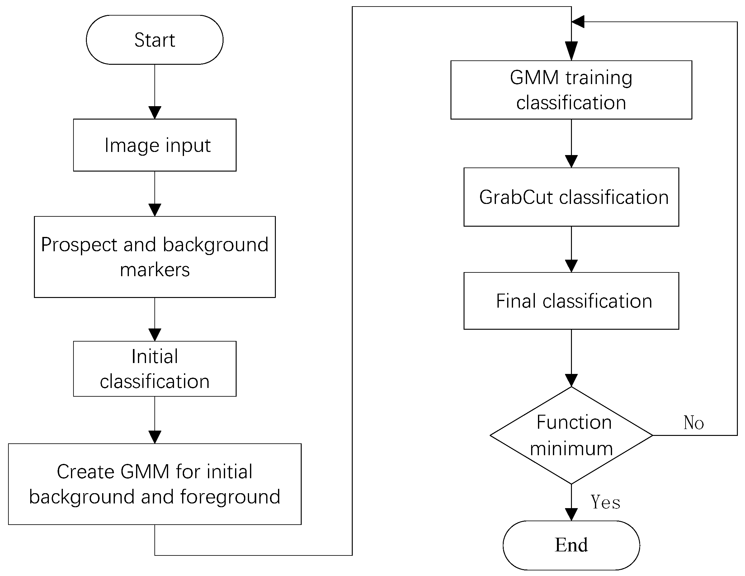
The GrabCut segmentation algorithm is an improvement of the GraphCut algorithm. The GrabCut algorithm utilizes texture (color) information and boundary (contrast) information in the image to interact with users through rectangular boxes, estimating foreground pixels inside the box and background pixels outside the box. After multiple iterations, it achieves target segmentation. The segmentation process of the algorithm is illustrated in Figure 1 [14].
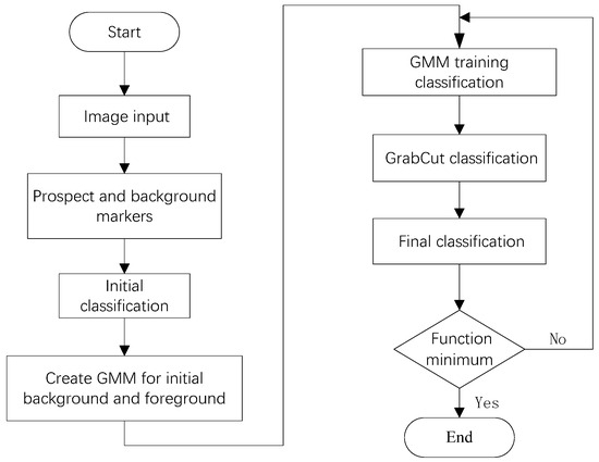
Figure 1.
Flowchart of the GrabCut algorithm.
The classic interactive image segmentation algorithm GrabCut achieves iterative optimization during the segmentation process, simplifies the required user interaction for segmenting objects, and uses a rectangular bounding box to estimate foreground pixels within the box and background pixels outside it [12].
The GrabCut energy function E is defined as follows:
The function represents the regional data term of the energy function, where is a histogram model, represents the transparency coefficient, 0 is the background, and 1 is the foreground, represents a single pixel, and the is defined as:
The smoothing item is:
Among them, C is the set of adjacent pixel pairs, is the Euclidean distance between adjacent pixels, and the selection of ensures appropriate switching between high contrast and low contrast in the exponential direction, which promotes consistency in similar grayscale regions. When the constant , the smoothness term is simply the well-known Ising prior, encouraging smoothness everywhere, to a degree determined by the constant [10].
This energy encourages coherence in regions with a similar grey-level. In practice, good results are obtained by defining pixels to be neighbors if they are adjacent either horizontally/vertically or diagonally (eight-way connectivity). When the constant β = 0, the smoothness term is simply the well-known Ising prior, encouraging smoothness everywhere, to a degree determined by the constant γ. It has been shown, however, that it is far more effective to set β > 0 as this relaxes the tendency to smoothness in regions of high contrast [10].
The GrabCut image segmentation process is as follows.
Initialization. The user obtains an initial trimap image T by directly selecting the target, where all the pixels outside the box are used as background images and all the pixels inside the box are considered as pixels that may be the target.
When , initialize the label of pixel n, ; when , initialize the label of pixel n, .
The Gaussian Mixture Model (GMM) for background and foreground is initialized with and , respectively. The pixels belonging to the target and background are then clustered into k categories that correspond to k Gaussian models in the GMM using the k-means algorithm.
The iterative minimization process is as follows:
- (1)
- Assign Gaussian components in the GMM to each pixel. For each in , .
- (2)
- For the given image data Z, iteratively optimize the parameters of GMM: .
- (3)
- Estimated segmentation (based on the Gibbs energy term analyzed in (1), establish a graph and calculate the weights t-link and n-link, and then use the max flow/min cut algorithm for segmentation).
- (4)
- Repeat the above process until convergence occurs.
- (5)
- Use border cutout. Use border matching to smooth and perform post-processing on the segmented boundaries.
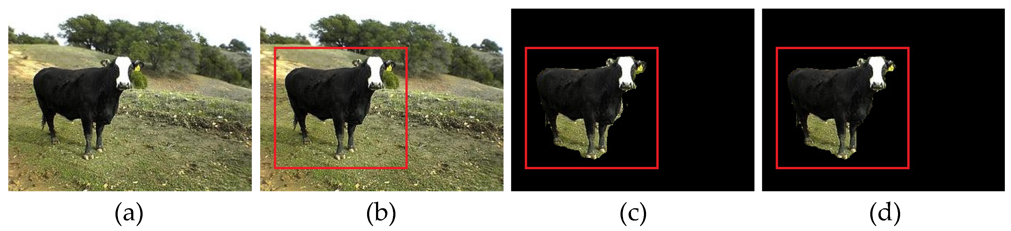
Figure 2 shows the segmentation process of the GrabCut algorithm: (a) shows the original input image, (b) shows the user interaction process, selecting the segmentation target with a red rectangular box, (c) is the segmentation result of one iteration of GrabCut, and (d) is the segmentation result of 30 iterations. The GrabCut algorithm refines segmentation by selecting the target object in the image and iterating multiple times until the desired segmentation result is achieved.
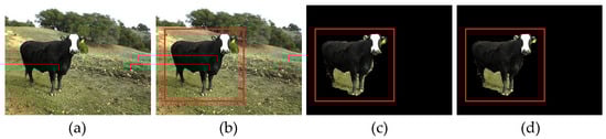
Figure 2.
GrabCut segmentation algorithm example. (a) Original image, (b) Target selection, (c) One iteration segmentation, (d) 30 iterations segmentation.
2.2. Description of the Problem
From the above introduction and examples of the GrabCut algorithm, it is evident that GrabCut selects the target object in the image and iteratively segments it until the segmentation meets the desired criteria and completes the segmentation process.
The GrabCut algorithm starts by estimating the position of the foreground object in the image using a rectangular box, with the area outside this box treated as background. However, depending solely on this rectangular box can lead to inaccuracies, particularly when dealing with objects with complex shapes or intricate boundaries. This approach may result in segmentation outcomes that do not meet precise requirements, as illustrated in Figure 2, where the segmentation result lacks precision.
In order to improve segmentation accuracy, the GrabCut algorithm requires multiple iterations, especially for high-resolution images or large datasets, where multiple iterations result in slow segmentation speed.
3. Algorithm Improvement
By introducing an appearance overlap term to optimize segmentation energy function, the GrabCut algorithm achieves optimal segmentation with just one iteration. This approach addresses the inaccuracies associated with using rectangular boxes for segmentation. The interactive method based on seeds is used to improve segmentation accuracy, especially for complex objects, thereby enhancing the overall effectiveness of the algorithm.
3.1. Appearance Overlap in Minimum Cutting
Assuming S is a part of all pixel sets C, denoted as , and are used to represent non-standardized color histograms on the appearance of the image foreground and background, respectively. The pixels belonging to bin in the image are defined as ; and represent the number of pixels in the foreground and background of bin , respectively. The appearance overlap term is used to evaluate the communication of foreground and background bin counts by combining simple and effective terms into an energy function, as follows:
For a better explanation, we will rewrite as:
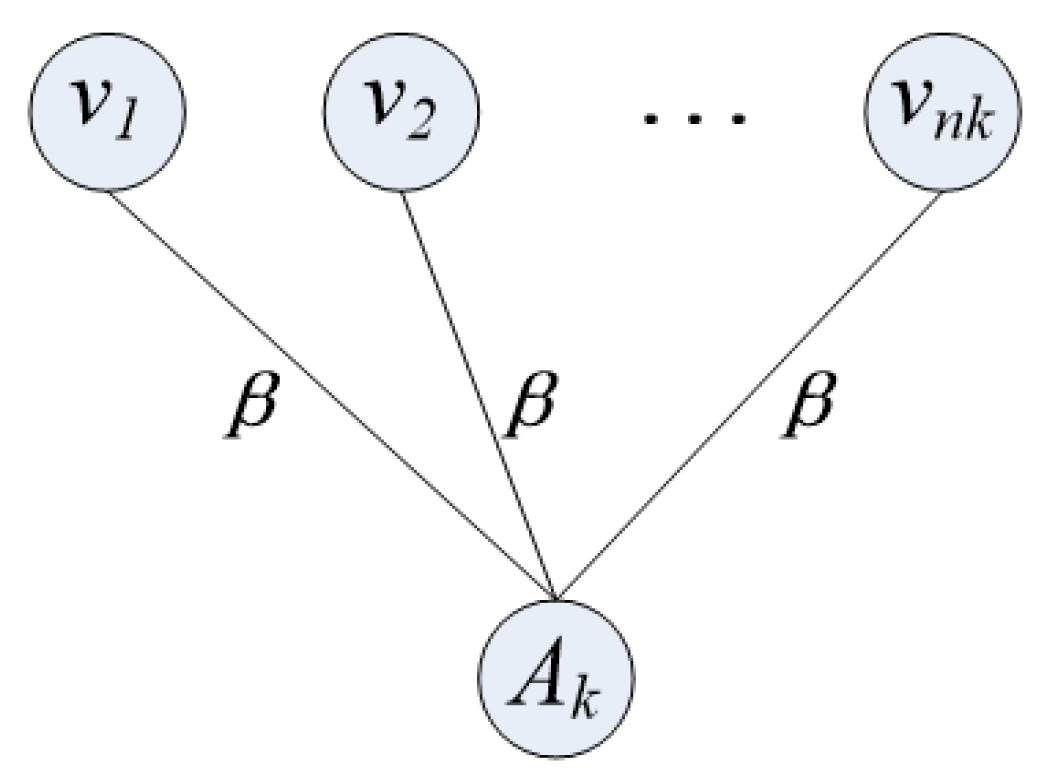
Figure 3 shows the construction details of the above expression.

Figure 3.
Graph construction of .
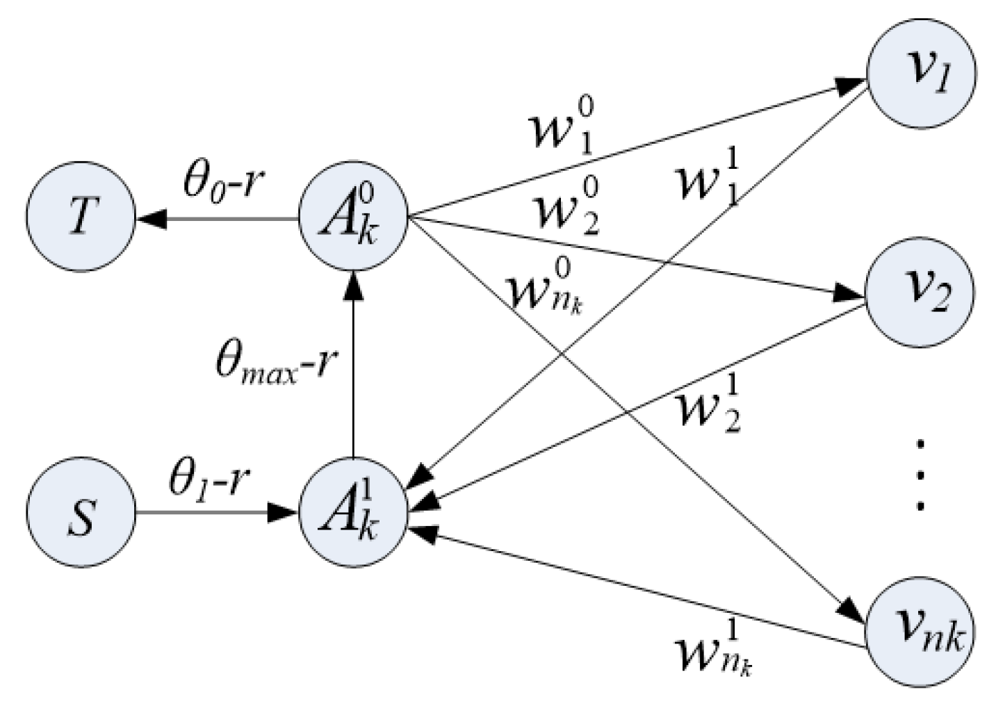
The node in the figure corresponds to the pixel in the bin and is connected to the auxiliary node using an undirected line segment. In the figure, represents the weight of these appearance overlapping items when linked, and .
auxiliary nodes are added in the figure and auxiliary nodes belonging to bin are connected. In this way, each pixel in the graph is connected to its corresponding auxiliary node. The weight of these connections is set to 1. Bin is divided into foreground and background; the corresponding pixel results are and . So, when cutting and separating foreground and background pixels, it is necessary to cut the number of pixels connected to the auxiliary node in bin , with the number of cut connections being or . The optimal number of cuts must be determined by selecting in (5).
Kohli and Torr’s research has proposed a similar graph construction to minimize the following forms of the high-order Pseudo Boolean function [15]:
In the equation, is a binary variable in set ; , ; and parameters , , and satisfy the constraint conditions and . Equation (6) can be used for minimization, and its minimization process is as follows:
Treat each color bin as a set and set the weight parameters , , in addition to , , , where is the number of pixels in the bin. Reduce to through parameter settings. Compared to other graph constructions, our graph construction has an advantage in the construction of auxiliary nodes; that is, compared to two auxiliary nodes, we only need one bin per bin [15]. In addition, our structure also uses the Pseudo Boolean function whose directed connection is extended to Equation (6). Its structure is shown in Figure 4; .
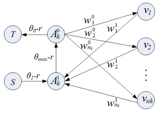
Figure 4.
The graph construction for minimizing Pseudo Boolean function.
To explain its principle, we considered four possible allocations of auxiliary nodes and . Table 1 lists the four possible allocations and the associated costs of the corresponding parts of the segmentation process. Minimum segmentation is used to optimize Equation (6). The optimal segmentation must choose the value with the lowest segmentation cost among the four allocations in the table to minimize Equation (6).

Table 1.
The cost of corresponding cuts.
Unlike what we constructed, the methods in the literature require , and the parameter in should meet the following constraints:
In contrast, we can use any meeting the above conditions to optimize the higher-order function in Equation (6), but the prerequisite must be and .
3.2. Energy Optimization Based on Appearance Overlap
We have improved the binary segmentation in GrabCut by citing the appearance overlap penalty. It is used in such a way that the user selects the target with a rectangular box around the target of interest in the image, and then segments the binary image in the rectangular box. The pixels outside the rectangular frame are background pixels. Assuming is the binary mask corresponding to the bounding box, is the ideal segmentation effect for the target, is the actual segmentation effect, and is the set of image pixels, where , , . The the segmentation energy function based on rectangular box interaction is:
The first item in the equation is within the bounding box , the second item is the appearance overlap penalty item, and the last item is the smoothing item, where is a constant. The average value of the image is set by and . This energy can be optimized through a single image segmentation.
It is common to adjust the relative weights of each energy term for a given dataset [16]. The rectangular bounding box should contain useful information about the target for segmentation. We use the measure of appearance overlap between the rectangular box and the background outside the box to dynamically search for the specific relative weight of the appearance overlap item relative to the image of the first item in Equation (8). In our segmentation algorithm, we adaptively set image specific parameters based on the information within the user-defined border, which are defined as follows:
In the formula, is the global parameter tuned for each application. Compared with the relative weight , is more robust.
In seed-based interactive segmentation, due to the strict constraints imposed by the user between the target and background, there is no need for volume balancing. Therefore, the energy function is:
3.3. Significant Object Segmentation
The detection and segmentation of salient regions of target objects is an important preprocessing step for object recognition and repair. Obvious objects usually have a different appearance from the background [17,18,19]. We use the contrast-based salient region detection filter provided in the literature [18] to filter images, as it produces the best accuracy when setting thresholds and comparing them with real targets. Let represent the normalized saliency map and be its average. The segmentation energy function is:
We define energy terms with and without appearance overlap, respectively. We define as the energy term that combines significance and smoothness:
We define as an energy item with appearance overlap:
The structure shown in Figure 3 is used to optimize during one-time graphic cutting.
4. Experimental Analysis
4.1. Algorithm Comparison Experiments
The target segmentation images used in the algorithm comparison experiment come from the Stanford background dataset released by the Stanford DAGS Laboratory [20]. The dataset contains 715 scenic images from rural and urban areas selected from the public datasets LabelMe, MSRC, PASCAL VOC and Geometric Context. We divide the images in the dataset into single target simple image and multi-target complex image, and use min_cut, GrabCut and improved GrabCut algorithm for segmentation experiments respectively. The results of segmentation experiments were analyzed qualitatively and quantitatively.
We selected images from various scenarios in the database, such as (4) in Figure 5 and (7) and (8) in Figure 6. In (4), a part of the animal’s leg is partially covered by green grass, but not completely obscured. In (7), the colors of the animal’s head and the background are very similar. And in (8), only a small portion of the animal in the corner is visible. These situations will affect the segmentation results. However, at the same time, the segmentation results can better reflect the performance of the algorithm.

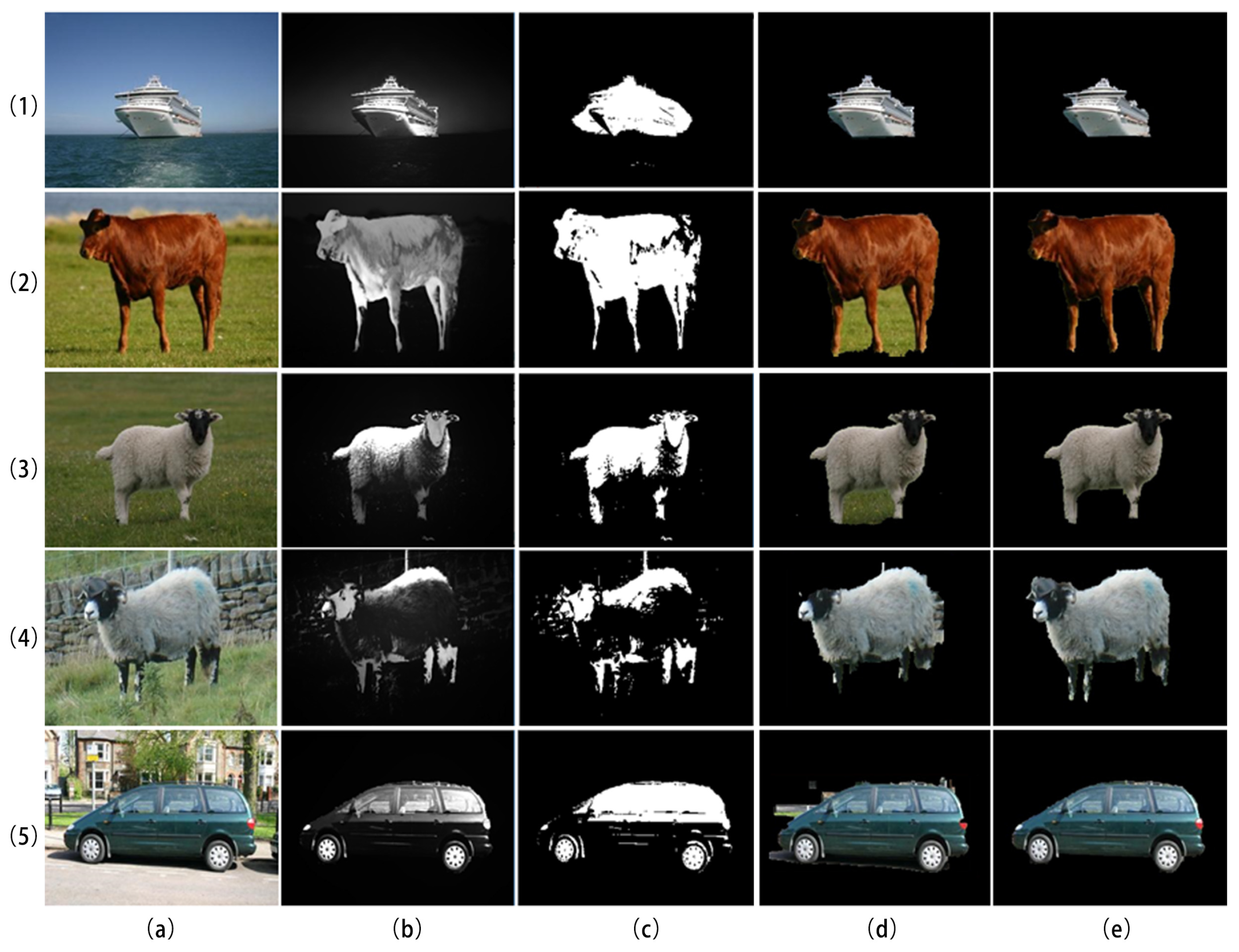
Figure 5.
Comparison of single-target segmentation results. (a) Original input image, (b) salient object detection result, (c) binary image after using min_cut segmentation on the salient image, (d) result of 20 iterations of GrabCut algorithm segmentation, and (e) segmentation result of the improved GrabCut algorithm.
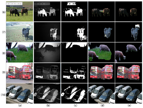
Figure 6.
Comparison of multi-target segmentation results. (a) Original input image, (b) salient object detection result, (c) binary image obtained after using min_cut segmentation on the salient image, (d) result of 20 iterations of GrabCut algorithm segmentation, and (e) segmentation result of the improved GrabCut algorithm.
Figure 5 shows a comparison of the segmentation effects of three algorithms on single target images.
Figure 6 shows a comparison of the segmentation results of three algorithms for multi-target images.
4.2. Qualitative and Quantitative Comparison
In order to better evaluate the segmentation effect, we have analyzed it from both qualitative and quantitative perspectives.
4.2.1. Qualitative Comparison
From Figure 5, it is evident that for the segmentation of a single target object, when the target is relatively simple, as depicted in line (1), all three methods successfully segment the object area, with GrabCut and the improved GrabCut algorithm yielding superior results. However, when the selected target object has a complex shape and significantly differs in color from the background, as seen in lines (2) and (3), the min_cut algorithm can outline the object but fails to highlight areas with darker pixels from salient object detection. This leads to rough segmentation results with unclear contours. GrabCut, while generally effective, sometimes mixes background parts, resulting in inaccurate segmentation.
In cases where the target object color is similar to the background, as shown in lines (4) and (5), the min_cut algorithm fails to segment the object entirely, while GrabCut only partially segments the target area with relatively rough contours. Comparatively, the improved algorithm demonstrates the best segmentation performance and accuracy across all scenarios.
Figure 6 compares the segmentation results of the three algorithms for multi-target images. The experimental results reveal that when the target object has a darker color significantly different from the background, as shown in line (6), both the min_cut and GrabCut algorithms can segment the object but with inferior results compared to the proposed algorithm. When certain object colors in multi-object images closely resemble the background, as in line (7), both min_cut and GrabCut algorithms may misclassify them as background, resulting in incomplete segmentation. Similarly, when the target object is lighter than the background, as depicted in line (8), the min_cut algorithm fails to segment it, and GrabCut achieves only partial segmentation. For complex target structures in lines (9) and (10), min_cut struggles to segment the object, while GrabCut provides segmented results with rough contours that lack smoothness.
Overall, the algorithm presented in this article excels in accurately segmenting multi-target objects across various conditions, demonstrating superior segmentation effectiveness.
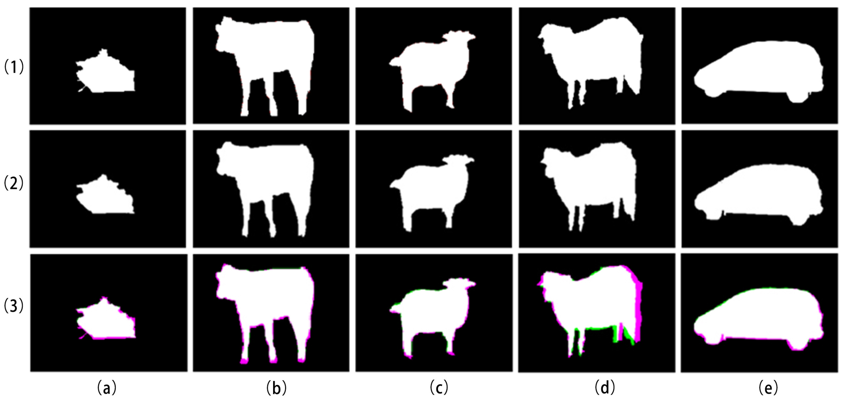
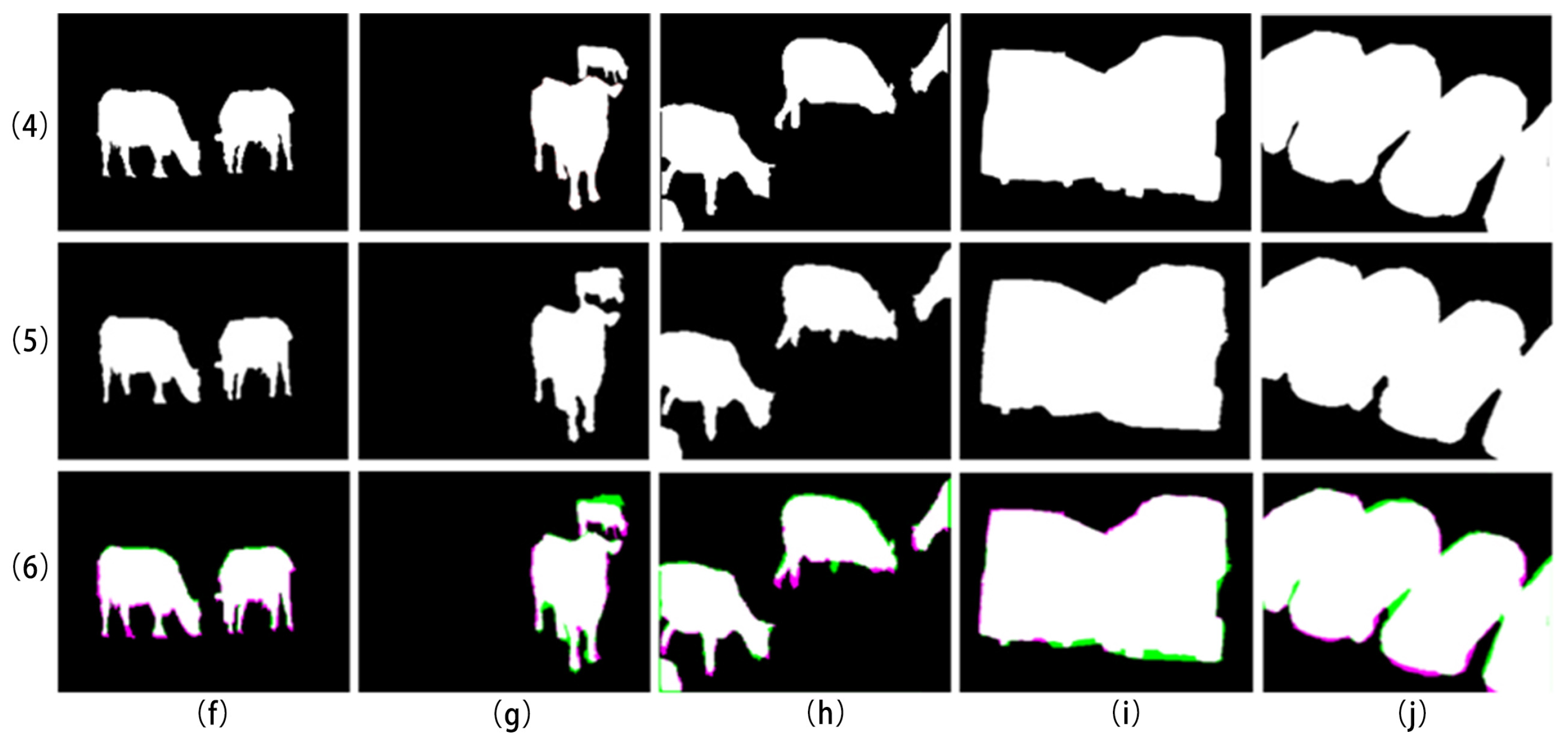
Figure 7 displays the residuals between the automatic segmentation results using the algorithm in this paper and the target images. Lines (1) and (4) in Figure 7 show the true value image of the original image. Lines (2) and (5) describe the true value images automatically segmented using the algorithm proposed in this paper, while lines (3) and (6) show the residuals between the automatic segmentation results of this paper and the target image.
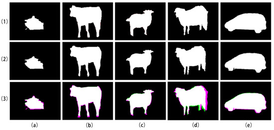
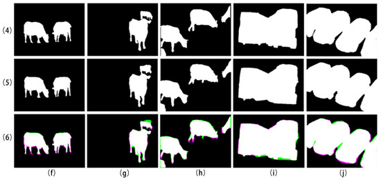
Figure 7.
The residual error between the automatic segmentation result and the target image. (1) The true value image of a single target original image, (2) the true value image automatically segmented from a single target image, (3) the residual image of single target image segmentation, (4) the true value image of a multi-target original image, (5) the true value image automatically segmented from a multi-target image, and (6) the residual image of multi-target image segmentation.
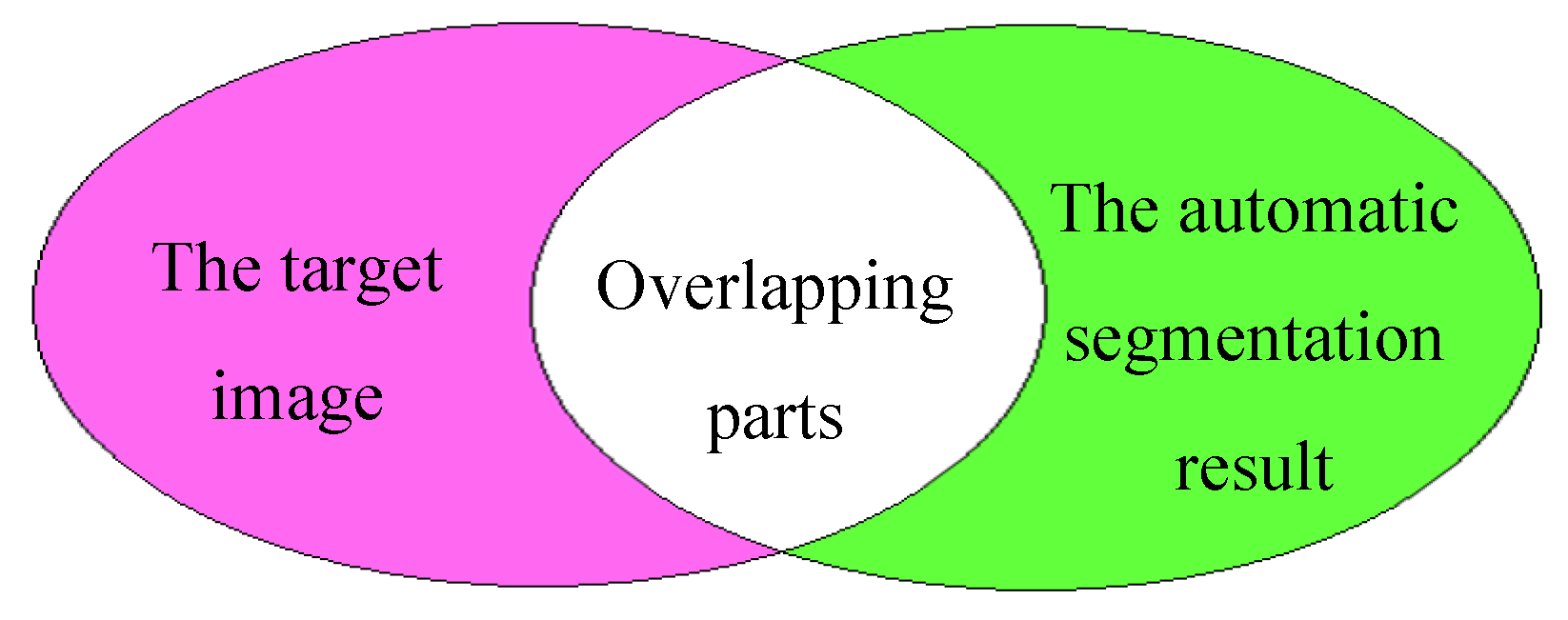
As shown in Figure 8, in the residual images, red indicates the original target image, green represents the automatic segmentation image from this paper, and white denotes overlapping regions.

Figure 8.
Residual plot example.
From the residual image, it can be intuitively observed that in columns (d), (f), and (h), there are some differences in segmentation results due to the similarity in color of some areas between the target object and the background. However, for most scenes, our algorithm can achieve good automatic segmentation.
4.2.2. Quantitative Comparison
To quantify the segmentation results, six parameters are used in the analysis.
(1) Algorithm running time: The shorter the image segmentation time, the faster the segmentation rate.
(2) DSC: The DSC (Dice coefficient) is a statistical index used to measure the similarity between two sets, which is often used to calculate the similarity between two samples. Its value range is between 0 and 1. The closer the value is to 1, the more similar the two sets are. The closer the value is to 0, the more dissimilar the two sets are.
The calculation formula for the Dice coefficient is as follows:
where A and B represent two sets, respectively, and represent the number of elements in sets A and B, and represents the number of intersection elements in sets A and B.
In this paper, A stands for the anticipated set of pixels and B represents the actual image’s target object. TP, FP, TN, and FN stand for true positives, false positives, true negatives, and false negatives, respectively.
(3) IoU: Intersection over Union (IoU) is an index used to evaluate the performance of target detection algorithm, which is often used in image segmentation tasks. It measures the degree of overlap between the predicted bounding box and the real bounding box. The number of pixels common between the measurement target and the prediction mask is measured and divided by the total number of pixels present on both masks.
IOU is defined as the intersection area of the predicted bounding box and the real bounding box divided by their union area. The specific calculation formula is as follows:
Among them, is the area of the intersection of the predicted boundary box and the real boundary box, and is their overall area.
The value of IOU ranges from 0 to 1. The larger the value, the higher the degree of overlap between the predicted result and the real result, that is, the more accurate the segmentation result.
(4) Pixel accuracy: Pixel accuracy is an index used to evaluate the performance of models in image segmentation tasks. It measures the ratio between the number of pixels correctly classified by the model at the pixel level and the total number of pixels. The calculation formula is as follows:
Specifically, it calculates the number of pixels that exactly match the real label in the model prediction result and divides it by the total number of pixels to obtain a score between 0 and 1. The closer the score is to 1, the more consistent the predicted result of the model is with the real label, that is, the better the performance of the model.
(5) Precision: Precision is defined as the fraction of automatic segmentation boundary pixels that correspond to ground truth boundary pixels. The precision can be calculated using the following formula:
The value range of precision is between 0 and 1. The higher the value, the higher the proportion of real cases in the samples predicted by the model as positive cases, that is, the more accurate the prediction of the model is.
(6) Recall: The recall is defined as the percentage of ground truth boundary pixels that were correctly identified by automatic segmentation. Recall is a measure of the proportion of positive image samples accurately classified as positive compared to the total number of positive image samples. Recall can be calculated using the following formula:
It is a measure of how well the model can identify positive samples. The higher the recall, the more positive samples are detected.
Table 2 compares the segmentation run times of the three algorithms for the target objects in Figure 5, and the average time taken to calculate the GrabCut algorithm is 20 iterations.
Table 2.
Algorithm runtime comparison.
From the experimental results, GrabCut requires the longest segmentation time, followed by min_cut, and the AO-GrabCut algorithm requires the shortest segmentation time. In addition, because image (4) is different from the other four pictures, its target object is similar to the background color, so the segmentation time of image (4) for each algorithm is longer than the other four pictures. It can be concluded that for pictures with similar front and background colors, segmentation takes longer. Judging from the overall results of the experiment, GrabCut requires the longest segmentation time, followed by min_cut, while the AO-GrabCut algorithm requires the shortest segmentation time among the three algorithms, and the segmentation time is controlled within 1 s. The AO-GrabCut algorithm has an average segmentation speed improvement of about 3.6 s compared to the min_cut algorithm and an average improvement of about 4.8 s compared to the GrabCut algorithm.
Table 3 shows the comparison of the segmentation running times of the three algorithms for the target objects in each image in Figure 6. The time taken to calculate the GrabCut algorithm is the average time of 20 iterations. Judging from the experimental results, similar to single target segmentation, GrabCut segmentation requires the longest time in multi-target segmentation, followed by min_cut, while the AO-GrabCut algorithm requires the shortest segmentation time, and the segmentation takes less than 1 s. The segmentation speed of AO-GrabCut algorithm is on average 3.5 s faster than min-cut algorithm and about 5 s faster than GrabCut algorithm.
Table 3.
Algorithm running time comparison.
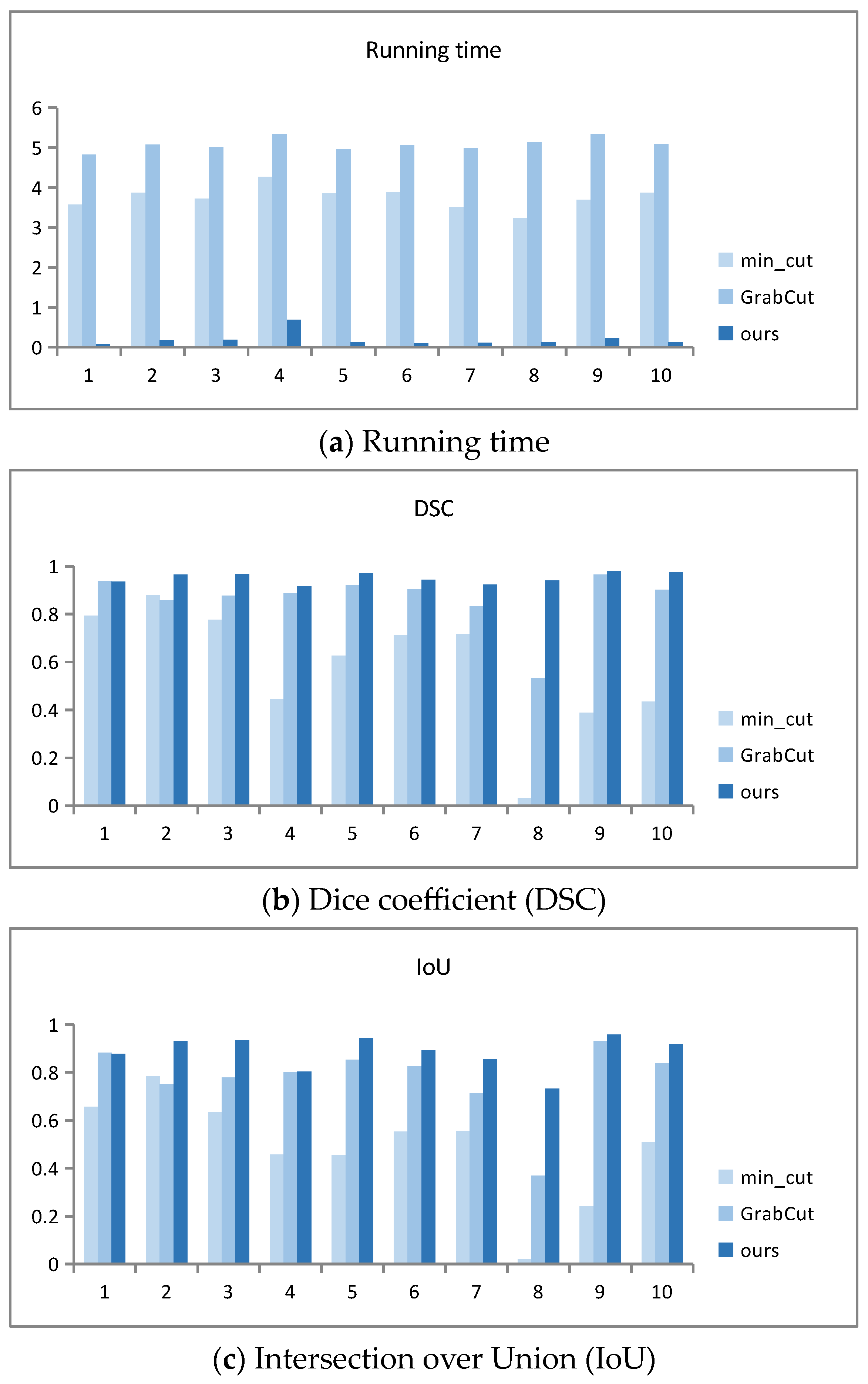
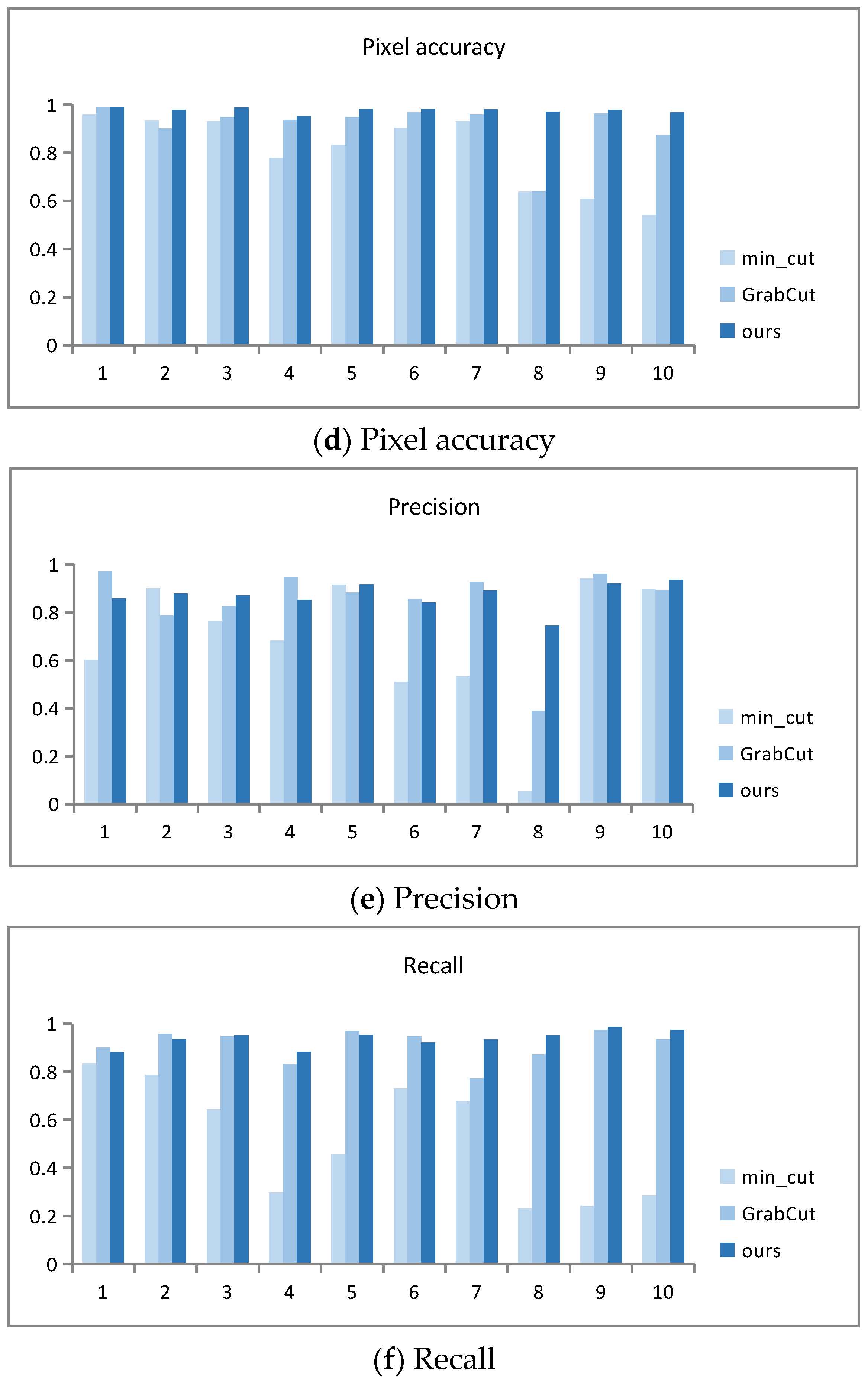
The running time data graphs in Figure 9 intuitively reflect the comparison of the running times for segmenting 10 target images using three algorithms. Among the three algorithms, GrabCut has the longest running time, and the improved segmentation algorithm AO-GrabCut has the shortest time and faster segmentation.
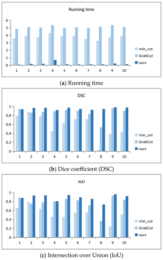
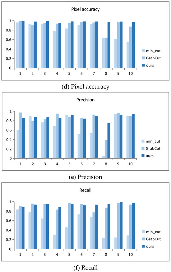
Figure 9.
Quantitative comparison results.
Table 4 shows the analysis data of the Dice coefficient (DSC), Intersection over Union (IoU), pixel accuracy, precision, and recall.
Table 4.
Quantitative analysis of data.
Figure 9 shows a bar chart of the analysis results for the Dice coefficient (DSC), Intersection over Union (IoU), pixel accuracy, precision, and recall.
From Figure 9b,c, it is evident that both GrabCut and the improved segmentation algorithm presented in this paper achieve larger values, indicating a higher degree of overlap between the automatically segmented images and the target images. Specifically, images (1), (4), and (9) show very close DSC and IOU values. For the remaining images, the improved algorithm consistently outperforms GrabCut, demonstrating significantly higher DSC and IOU scores. This indicates that the segmented images from the improved algorithm closely match the target images with greater overlap.
The pixel accuracy data graph in Figure 9d reveals that both GrabCut and the proposed algorithm achieve higher pixel accuracy, with a larger proportion of correctly segmented pixels. Images (1), (4), (6), (7), and (9) exhibit closely matched pixel accuracy values. However, for other images, the improved algorithm consistently achieves significantly higher pixel accuracy compared to GrabCut, indicating a higher proportion of accurately segmented pixels in the resulting images.
The precision and recall data graphs in Figure 9e,f show that the precision and recall values of the improved segmentation algorithm and GrabCut are larger, indicating a higher proportion of correctly segmented objects. Each algorithm shows its strengths in different scene segmentation tasks. GrabCut exhibits varying levels of correct segmentation proportions across different scene images, whereas the improved algorithm in this paper consistently delivers stable segmentation results across various scene images.
Overall, the graphs illustrate that the improved segmentation algorithm outperforms GrabCut in terms of DSC, IOU, pixel accuracy, precision, and recall across a range of image segmentation tasks, showcasing its superior performance and stability in achieving accurate and reliable segmentation results.
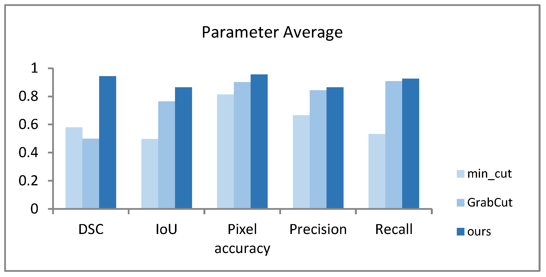
Table 5 shows the segmentation of 715 images from the Stanford background dataset using min_cut, GrabCut, and our AO-GrabCut algorithm. The average values of the parameters DSC, IoU, pixel accuracy, precision, and recall were quantitatively analyzed.
Table 5.
Average value of quantitative analysis parameters.
From the average values of quantitative parameters in outlined Table 5 and Figure 10, it can be seen that among the three algorithms min_cut, GrabCut, and AO-GrabCut, the min_cut algorithm has a lower segmentation accuracy, while the GrabCut algorithm significant differs in segmentation performance and poor stability for different images. The various parameters of the AO-GrabCut algorithm have improved compared to the min_cut and GrabCut algorithms, and the accuracy and stability of the algorithm are better.
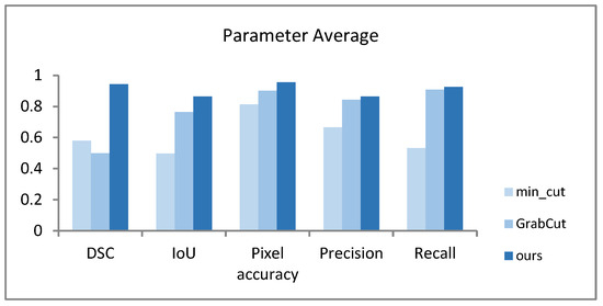
Figure 10.
Average values of quantitative analysis parameters.
5. Conclusions
GrabCut, as a classic image segmentation method, requires multiple iterations to achieve satisfactory segmentation results when dealing with complex structures and minimal color differences between the target object and its surroundings. Addressing issues with GrabCut, the article introduces an appearance overlap term to optimize segmentation energy, achieving optimal segmentation results in a single iteration. This improvement enhances overall segmentation speed without compromising accuracy. For single target simple images, AO-GrabCut has an average segmentation speed improvement of about 3.6 s compared to the min_cut algorithm and an average improvement of about 4.8 s compared to the Grabcut algorithm. For complex images with multiple targets, the segmentation speed of the AO-GrabCut algorithm is on average 3.5 s faster than min-cut algorithm and about 5 s faster than the GrabCut algorithm. Compared to GrabCut, AO-GrabCut has an average segmentation speed that is approximately 25 times faster. Compared to min_cut, the average segmentation speed of AO-GrabCut is approximately 19 times faster. At the same time, experiments have shown that the AO-GrabCut algorithm has more stable segmentation performance in various scene segmentation scenarios.
Furthermore, the article enhances GrabCut through a seed-based interactive approach instead of relying solely on bounding boxes. Users can directly provide seed points on the image to more accurately indicate foreground and background regions. This interactive method not only strengthens the algorithm’s ability to accurately segment complex objects but also simplifies the user experience.
Author Contributions
Methodology, S.P., T.H.G.T. and F.L.S.; Software, Y.X.; Validation, M.C. All authors have read and agreed to the published version of the manuscript.
Funding
This work was supported by the Opening Project of Sichuan Province University Key Laboratory of Bridge Non-destruction Detecting and Engineering Computing, grant number 2023QYY07.
Data Availability Statement
Data are contained within the article.
Conflicts of Interest
The authors declare no conflicts of interest.
References
- Han, S.; Wang, L. Overview of Threshold Methods for Image Segmentation. Syst. Eng. Electron. Technol. 2022, 102, 91–94. [Google Scholar]
- Jiang, F.; Gu, Q.; Hao, H. Overview of Content based Image Segmentation Methods. J. Softw. 2017, 28, 160–183. [Google Scholar]
- Hao, Q.; Zheng, W.; Wang, C.; Xiao, Y.; Zhang, L. MLRN: A multi-view local reconstruction network for single image restoration. Inf. Process. Manag. 2024, 61, 103700. [Google Scholar] [CrossRef]
- Yue, G.; Li, Y.; Jiang, W.; Zhou, W.; Zhou, T. Boundary Refinement Network for Colorectal Polyp Segmentation in Colonoscopy Images. IEEE Signal Process. Lett. 2024, 31, 954–958. [Google Scholar] [CrossRef]
- Kalb, T.; Beyerer, J. Principles of Forgetting in Domain-Incremental Semantic Segmentation in Adverse Weather Conditions. In Proceedings of the IEEE/CVF Conference on Computer Vision and Pattern Recognition, Vancouver, BC, Canada, 17–24 June 2023; pp. 19508–19518. [Google Scholar]
- Khan, K.; Khan, R.U.; Ahmad, F.; Ali, F.; Kwak, K.-S. Face Segmentation: A Journey From Classical to Deep Learning Paradigm, Approaches, Trends, and Directions. IEEE Access 2020, 8, 58683–58699. [Google Scholar] [CrossRef]
- Li, C.; Sun, C.; Wang, J. Leaf vein extraction method based on improved Sobel operator and color tone information. J. Agric. Eng. 2011, 27, 196–199. [Google Scholar]
- Hu, M.; Li, M.; Wang, R. Application of an improved Otsu. J. Electron. Meas. Instrum. 2010, 24, 443–449. [Google Scholar] [CrossRef]
- Zhao, Y.; Liu, J.; Li, J. Medical image segmentation. Comput. Eng. Appl. 2007, 238–240. [Google Scholar]
- Boykov, Y.Y.; Jolly, M.P. Interactive graph cuts for optimal boundary & region segmentation of objects in ND images. In Proceedings of the Eighth IEEE International Conference on Computer Vision, ICCV 2001, Vancouver, BC, Canada, 7–14 July 2001; Volume 1, pp. 105–112. [Google Scholar]
- Boykov, Y.; Kolmogorov, V. An experimental comparison of min—Cut/max—Flow algorithms for energy minimization in vision. Tissue Eng. 2005, 26, 1631–1639. [Google Scholar]
- Rothe, C.; Kolmogorov, V.; Blake, A. “GrabCut”—Interactive foreground extraction using iterated graph cuts. ACM Trans. Graph. 2004, 23, 309–314. [Google Scholar] [CrossRef]
- Liang, Y.; Li, S.; Liu, X.; Li, F. GrabCut algorithm for automatic segmentation of target leaves in complex backgrounds. J. S. China Norm. Univ. Nat. Sci. Ed. 2018, 50, 112–118. [Google Scholar]
- Ruzon, M.; Tomasi, C. Alpha estimation in natural images. In Proceedings of the IEEE Conference on Computer Vision and Pattern Recognition, CVPR 2000 (Cat. No. PR00662), Hilton Head Island, SC, USA, 13–15 June 2000; Volume 1, pp. 18–25. [Google Scholar]
- Kohli, P.; Torr, P.H. Robust higher order potentials for enforcing label consistency. Int. J. Comput. Vis. 2009, 82, 302–324. [Google Scholar] [CrossRef]
- Vicente, S.; Kolmogorov, V.; Rother, C. Joint optimization of segmentation and appearance models. In Proceedings of the 2009 IEEE 12th International Conference on Computer Vision, Kyoto, Japan, 29 September–2 October 2009; pp. 755–762. [Google Scholar]
- Achanta, R.; Hemami, S.; Estrada, F.; Susstrunk, S. Frequency-tuned salient region detection. In Proceedings of the 2009 IEEE Conference on Computer Vision and Pattern Recognition, Miami, FL, USA, 20–25 June 2009; pp. 1597–1604. [Google Scholar]
- Cheng, M.M.; Mitra, N.J.; Huang, X.; Torr, P.H.S.; Hu, S.-M. Global contrast based salient region detection. IEEE Trans. Pattern Anal. Mach. Intell. 2014, 37, 569–582. [Google Scholar] [CrossRef] [PubMed]
- Perazzi, F.; Krähenbühl, P.; Pritch, Y. Saliency filters: Contrast based filtering for salient region detection. In Proceedings of the 2012 IEEE Conference on Computer Vision and Pattern Recognition, Providence, RI, USA, 16–21 June 2012; pp. 733–740. [Google Scholar]
- Gould, S.; Fulton, R.; Koller, D. Decomposing a scene into geometric and semantically consistent regions. In Proceedings of the 2009 IEEE 12th International Conference on Computer Vision, Kyoto, Japan, 29 September–2 October 2009; pp. 1–8. [Google Scholar]

Disclaimer/Publisher’s Note: The statements, opinions and data contained in all publications are solely those of the individual author(s) and contributor(s) and not of MDPI and/or the editor(s). MDPI and/or the editor(s) disclaim responsibility for any injury to people or property resulting from any ideas, methods, instructions or products referred to in the content. |
© 2024 by the authors. Licensee MDPI, Basel, Switzerland. This article is an open access article distributed under the terms and conditions of the Creative Commons Attribution (CC BY) license (https://creativecommons.org/licenses/by/4.0/).