Synthesis of High-Selectivity Two-Dimensional Filter Banks Using Sigmoidal Function

Abstract

This paper explores an application of the sigmoidal function—the complementary integral Gaussian error function (erfc(.))—in two-dimensional (2D) uniform and nonuniform filter bank synthesis. The complementary integral Gaussian error function graph represents a smooth low-pass filter magnitude response. A parameter changes the function slope and increases the magnitude response selectivity. The theory is applied to 2D band-pass filter banks. Exact expressions for the magnitude response parameters are determined. As a result, 2D uniform and nonuniform filter banks with very high selectivity and exact shapes are obtained. Three synthesis examples of 2D filter banks with circular and fan-shaped magnitude responses are provided. The theoretical exposition is supplemented with two examples of image analysis using 2D uniform and nonuniform filter banks. A procedure to reduce the computations in image analysis is proposed. A comparison of filter synthesis between Parks–McLellan’s 2D filters and the erfc(.) demonstrates the significantly shorter calculation time of the proposed method.

1. Introduction

The modern development of communications and digital signal processing is related to the exploration of new theoretical knowledge as well as the addition and improvement of existing ones. One area in this direction is the processing of a video image with 2D filter banks. Two-dimensional filter banks aim to decompose the image into subbands for precise and detailed analysis. Signal processing using 2D filter banks is useful in several technical areas, such as aerial and satellite imaging, medicine, automotive applications, radar imaging processing, fast feature extraction in real-time computer vision applications, assistance systems, autonomous driving vehicles, etc.

The theory of 2D filters and filter banks has been thoroughly and extensively developed in several books [1,2] and publications. There is a wide variety of 2D finite impulse response (FIR) and Infinite Impulse Response (IIR) filters with various shapes and characteristics. This diversity allows for image processing when solving specific cases such as face recognition, fingerprint recognition, the detection of specific details in a picture, edge detection, etc. In [3,4,5], comprehensive reviews of 2D filter synthesis are presented. Various methods are proposed: McClellan transform [6,7], classical approximations [8,9,10], genetic algorithms [11,12,13], etc.

Other relevant studies on efficient 2D filter and filter bank designs are presented in [14,15,16,17,18,19].

In [14], a single-parameter tunable 2D Farrow structure for 2D filter synthesis is proposed. The approach taken ensures a reduction in the hardware complexity without sacrificing the accuracy with a normalized root mean square error of less than 0.5%.

In [15], an efficient analytic design method for 2D zero-phase circular filter banks using 1D prototype filters is described. The authors propose an efficient method to reduce computational complexity.

In [16], an elliptic approximation-based design approach for the design of 2D recursive fan filters is proposed. The synthesis procedure gives a filter with a low number of coefficients and a low computational complexity.

In [17], the kth-order McClellan transformation for 2D FIR filter design is proposed. As a result, 2D filters with perfect circular symmetry are obtained.

In [18], a semi-definite programming method for linear-phase half-band diamond (DS) and fan-shaped 2D filters is proposed. The applied approach moderates the dimension for the design problem and facilitates the design.

In [19], 1D to 2D frequency mapping based on accurate approximations of the Gaussian function for directional 2D filters with adjustable parameters and high selectivity is described. The designed filters have accurate frequency responses, good directional selectivity, and high linearity at a relatively low order.

In [20], a theory for the directional decomposition and reconstruction of 2D filters is presented. The exact reconstruction of the signal is discussed.

Some publications describe different and innovative approaches to 2D and multidimensional filter bank synthesis [21,22,23,24,25].

In [21], a design technique based on the minimization of the squared error between the original signal and a low-resolution representation of it is proposed. The applied approach leads to efficient image compression and pattern representations at lower resolutions in image analysis.

In [22], an approach based on the pseudo-polar Fourier transform of one-dimensional filter banks for designing directional 2D filter banks with an arbitrary number of subbands is demonstrated.

In [23], an effective multiresolution image representation using a combination of a 2D quincunx filter bank and directional wavelet transform is presented. In applications on nonlinear approximation and image coding, the proposed filter bank has visual quality improvements and has a higher signal-to-noise resolution.

In [24], the problems of multidimensional filter bank synthesis are discussed. Based on an earlier one-dimensional work, the authors show that it is possible to have a large family of biorthogonal perfect reconstruction multidimensional (n-D) subband coding filter banks. A complete parameterization of such filters leading to design methods in 2D case is given.

In [25], pseudo-polar Fourier transform for 2D nonsubsampled nonuniform directional filter bank synthesis is described. By utilizing the geometry property of the pseudo-polar grid, the authors employ a 1D nonsubsampled nonuniform filter bank to obtain a set of nonuniform wedge-shaped subbands. During the design process, only 1D operations are involved, and thus, the difficulty encountered in the design of 2D fan filters is avoided.

In some specific cases, digital image processing applications lead to the creation of two-dimensional filter banks with specific properties and parameters [26,27,28].

In recent years, the theory of 2D filters and filter banks has been developed with innovative methods and approaches, as shown in publications [29,30,31].

Image super-resolution, as a computer vision task with in-depth research value, aims to restore a high-resolution image from a low-resolution observation. In this regard, in [29], a lightweight multi-scale feature selection network for efficient image super-resolution is proposed.

In [30], an equiripple approximation of the Gaussian function is used to perform an analytical design procedure for uniform and nonuniform 2D FIR circular filter banks. To reduce the computational complexity, polyphase decomposition for a 2D filtering operation with a large kernel size and block filtering with smaller size matrices are used.

In [31], the theory of H_∞ filter synthesis for 2D systems is described. The approach uses linear matrix inequalities to establish the conditions for the filter’s existence and convert the filter design problem into a convex optimization problem.

In [32,33], an efficient method for 2D filter synthesis using the sigmoidal function is proposed. In comparison with the above-described methods, the synthesis process is easy, and the obtained 2D finite impulse response (FIR) filters have very high selectivity, better than those of currently known 2D filters. It is demonstrated that the obtained filters with smooth magnitude responses possess better selectivity than Parks–McClellan’s filters with equiripple responses and lower computational complexity. In this paper, this 2D filter theory is applied to 2D FIR filter banks.

2. Theoretical Background

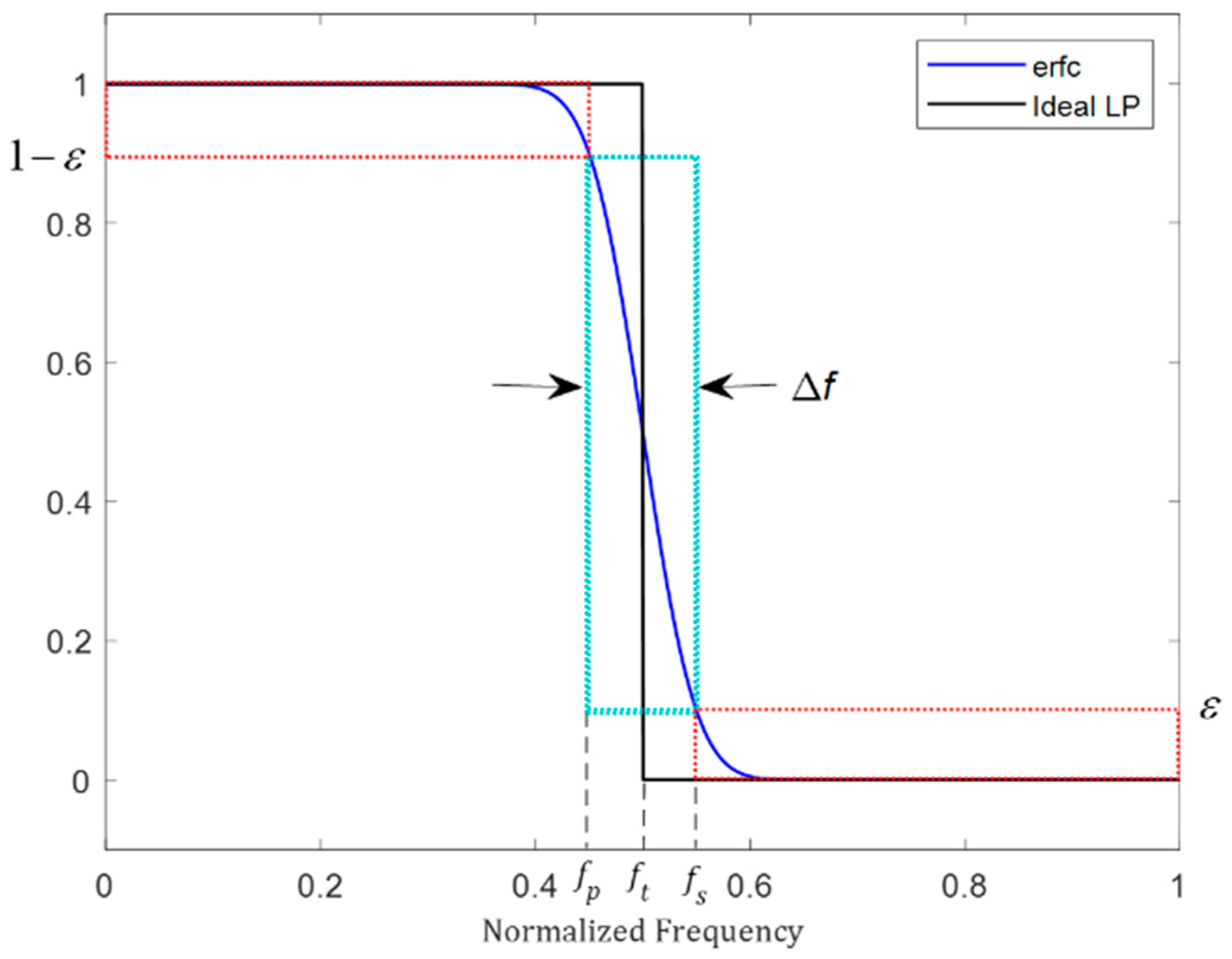
2.1. One-Dimensional Low-Pass Filter with Sigmoidal Function

Essentially, the graph of the sigmoidal function represents a low-pass filter magnitude response. In [34], a study of properties for some sigmoidal functions for FIR filter synthesis is presented, including the following: sigmoid, arctangent, hyperbolic tangent, power function (Butterworth), and complementary integral Gaussian error function (erfc(.)). It is proven that the magnitude response obtained using the erfc(.) has the best selectivity in comparison with the studied sigmoidal functions, because the erfc(.) approximates the ideal low-pass filter magnitude response with the smallest error.

In [35], a low-pass (LP) FIR filter with the complementary Gaussian error function (erfc(.)) is described. As was noted, the graph of the erfc(.) represents a low-pass filter magnitude response, as shown in Figure 1.

The LP magnitude response is determined by the expression

$$H\left(f\right)=0.5\mathrm{erfc}\left(2\beta \left(f-f_t\right)\right), f\in \left[0,1\right],$$

(1)

where f is a normalized frequency. The transition band Δf is limited by the stopband cut-off frequency f_s and passband cut-off frequency f_p, and f_t is the middle frequency of the transition band. The stopband attenuation is defined by the parameter ε, and the passband from the passband ripple is as follows: δ = 1 − ε. The parameter β is determined by the following condition: H(f_p) = δ. Increasing the parameter β changes the function slope gradient, which leads to a narrower transition band and better filter selectivity:

$$\beta ={\mathrm{erfc}}^{-1}\left(2\epsilon \right)/\Delta f,$$

(2)

where erfc⁻¹(.) is the inverse complementary integral Gaussian error function.

2.2. One-Dimensional Band-Pass Filter Prototype

In [36], the theory is extended to band-pass (BP) and band-stop (BS) filters. The change in the f_t value translates the function along the frequency axis. Thus, the magnitude response of the BP filter can be obtained as a combination of a high-pass filter with the mirror erfc(.) function in the range [0, f₀], and a low-pass filter (1) in the range [f₀, 1], where f₀ is the middle frequency of the BP filter. The magnitude response is given by the following expressions:

$$H_{BP}=\left\{\begin{array}{c}{H}_{HP}\left(f\right)=1-0.5\mathrm{erfc}\left(2\beta \left(f-f_{t\_HP}\right)\right);f\in \left[0, f_0\right]\\ H_{LP}\left(f\right)=0.5\mathrm{erfc}\left(2\beta \left(f-f_{t\_LP}\right)\right);f\in \left[f_0,1\right]\end{array}\right.$$

(3)

Figure 2 shows the BP filter magnitude response.

The magnitude response of the band-stop filter is easy to derive from

$$H_{BS}=1-H_{BP}$$

(4)

The BP filter bandwidth (BW) is defined at the magnitude response level δ = 1 − ε, as is shown in Figure 2. The obtained magnitude response is maximally flat, smooth, and without oscillations in the stop bands [35,36]. When ε is fixed, the BP filter selectivity depends on the parameter Δf, as shown in (2).

3. Two-Dimensional Filter Banks Synthesis

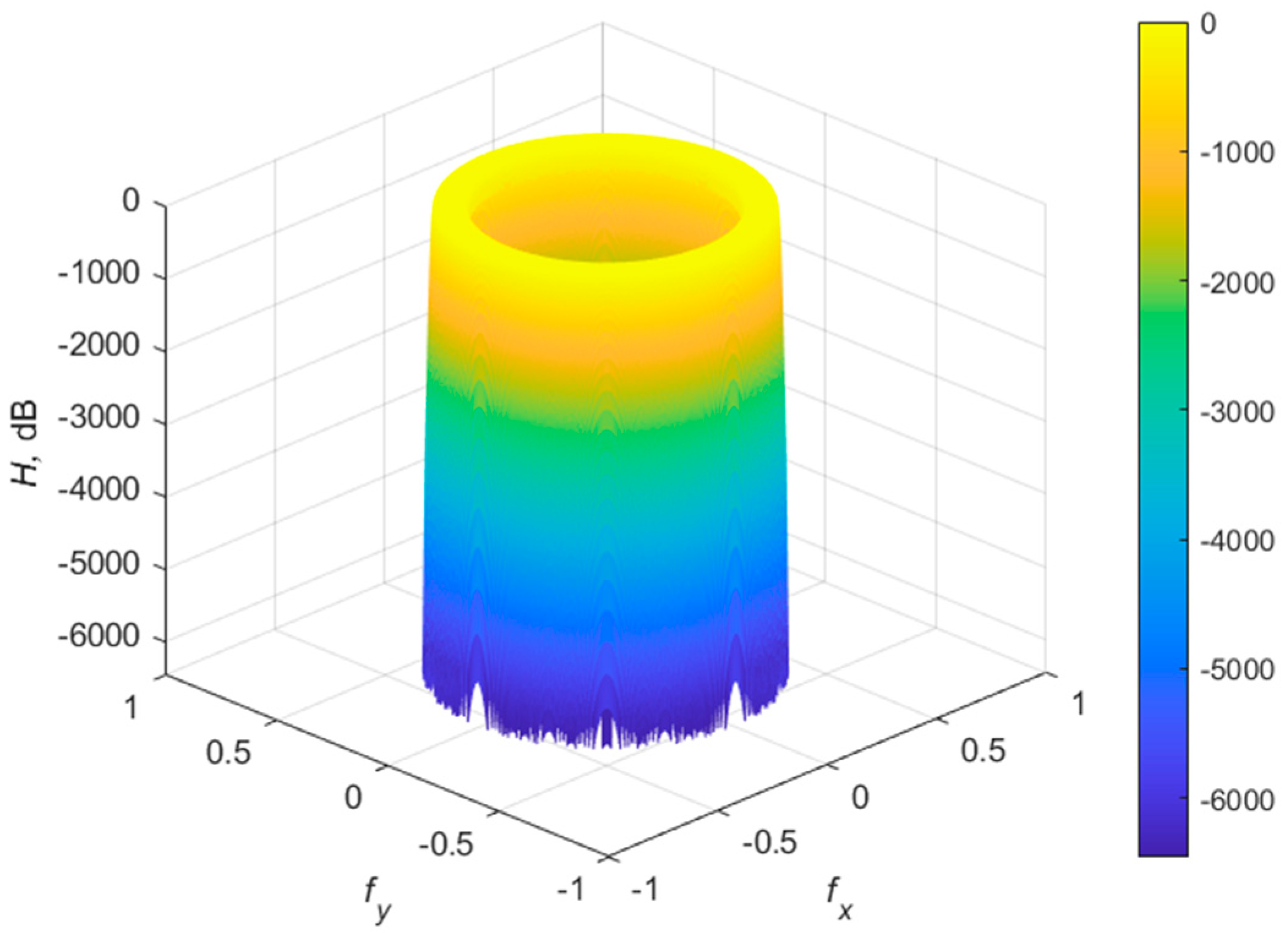
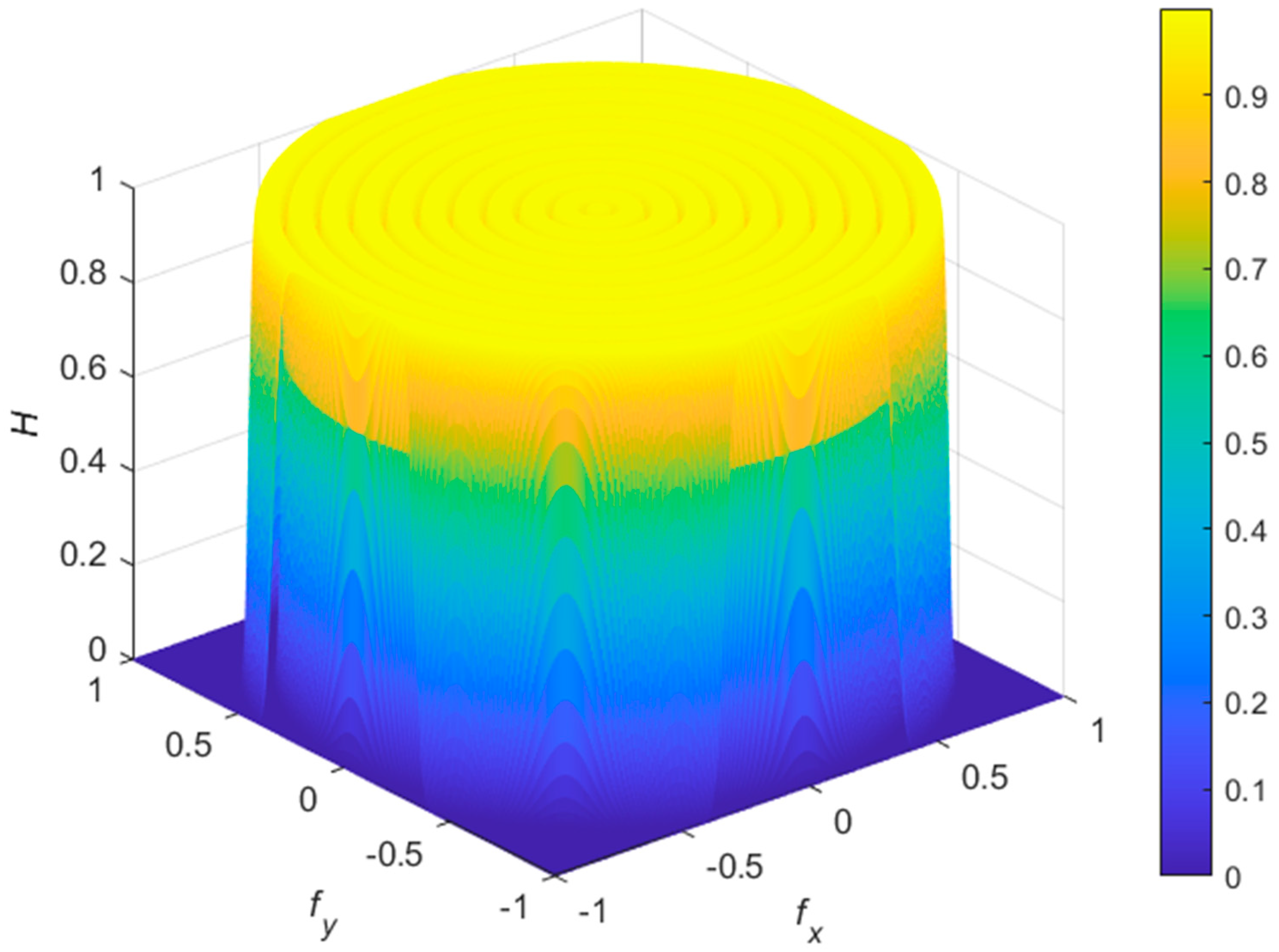
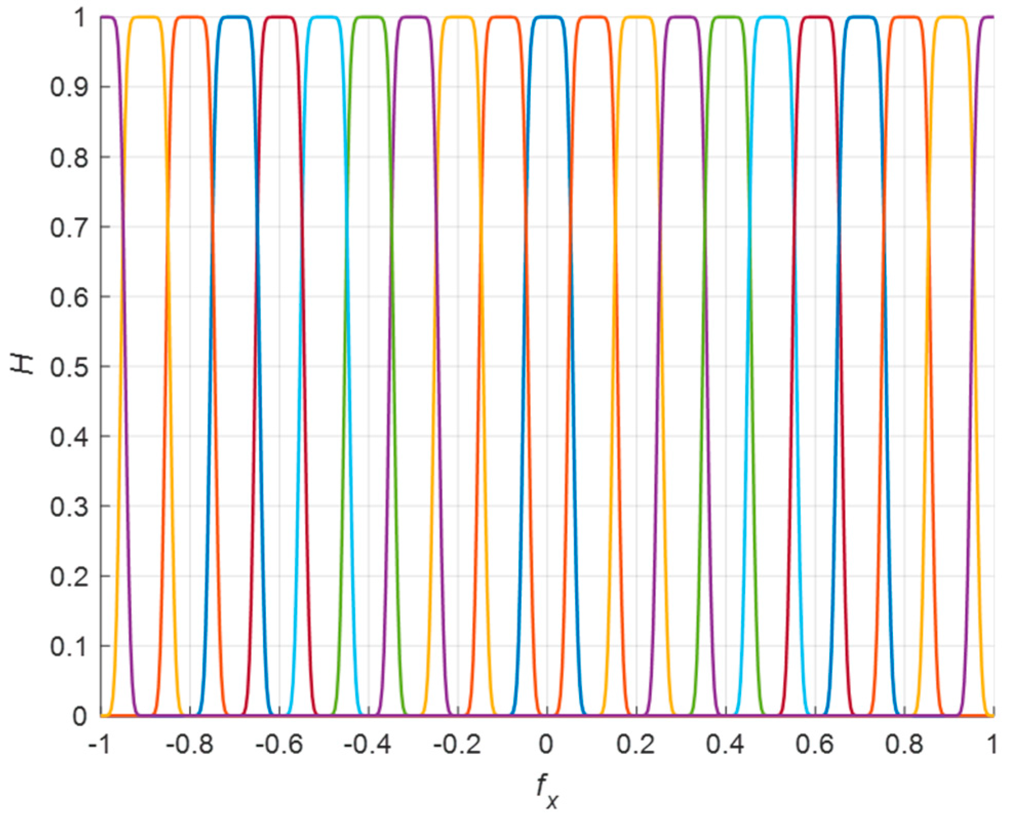
3.1. Two-Dimensional Uniform Filter Banks

In the synthesis process, we assume that the passband ripple is δ = 1 − ε = $1/\sqrt{2}$ = 0.7071, that is, level −3.01 dB. Thus, ε = 1 − $1/\sqrt{2}$. The argument f in (3) increases linearly in the range [0, 1]. For 2D filter synthesis, it is necessary to replace the argument with an x $\times$ y transformation matrix $R\left(f_x,f_y\right)$. x $\times$ y is the 2D filter size, and the variables f_x $\in$ [−1, 1], f_y $\in$ [−1, 1] define a normalized frequency space. By substituting $R\left(f_x,f_y\right)$ in (3), we obtain the 2D magnitude responses.

For a 2D filter with a circular shape, the transformation matrix is

$$R_{circle}=\sqrt{f_x^2+f_y^2},$$

(5)

thus,

$$H_{HP}\left(f_{x,}{f}_y\right)=1-0.5\mathrm{erfc}\left[2\beta \left(R_{circle}\left(f_{x,}{f}_y\right)-f_{t\_HP}\right)\right];$$

(6)

$$H_{LP}\left(f_{x,}{f}_y\right)=0.5\mathrm{erfc}\left[2\beta \left(R_{circle}\left(f_{x,}{f}_y\right)-f_{t\_LP}\right)\right]$$

(7)

The 2D band-pass filter magnitude response is obtained from the expression

$$H_{BP}\left(f_x,f_y\right)=H_{LP}\left(f_x,f_y\right)\times H_{HP}\left(f_x,f_y\right)$$

(8)

The proposed method produces 2D band-pass filters with extremely high selectivity. For example, in Figure 3 and Figure 4, a magnitude response H in dB of a 2D band-pass circular filter with BW = 0.1, f_t = 0.5, β = 385.3394, δ = −3.01 dB, Δf = 1/1000, and a grid size of 1024 × 1024 is shown.

Figure 4 shows the top view of the same magnitude response in dB. The 2D filter magnitude response represents a truncated conical body with dimensions defined from the filter parameters.

Example 1.

The realization of 11 stages of uniform-spaced filter banks with circular shapes with parameters: the number of stages is N = 11, the passband ripple is δ = $1/\sqrt{2}$, and the transition band is Δf = 0.01.

The component filters of the filter bank are concentric bodies, as shown in Figure 3, and overlapped at level $1/\sqrt{2}$ (−3.01 dB). The bandwidth is equal to

$$BW=1/\left(N-1\right)=0.1,$$

(9)

which makes 11 stages and 10 bandwidths. The first bank is a 2D LP filter with f₀₁ = 0 and a bandwidth of BW/2. The last bank is a 2D HP filer with f₀₁₁ = 1 and a bandwidth of BW/2. The remaining nine banks are 2D BP filters with bandwidths BW. Using (2), β = 38.5339 is calculated, and using (5), the R_circle value is calculated.

The magnitude responses are obtained using Equations (6)–(8).

$$H_{HPi}=1-0.5\mathrm{erfc}\left[2\beta \left(R_{circle}-f_{0i}+BW/2+\Delta f/2\right)\right];$$

(10)

$$H_{LPi}=0.5\mathrm{erfc}\left[2\beta \left(R_{circle}-f_{0i}-BW/2+\Delta f/2\right)\right];$$

(11)

$$H_i=H_{LPi}\times H_{HPi}, i=1,2,\dots ,N.$$

(12)

Figure 5 and Figure 6 show the 2D circular filter banks’ magnitude responses.

In Figure 6, a diametral cut of the 2D magnitude responses is plotted. All responses are overlapped exactly at level $1/\sqrt{2}$ (−3.01 dB).

Example 2.

Two-dimensional fan filter banks of arbitrary inclination are described as follows: the number of stages is N = 11, the passband ripple is $\delta =1/\sqrt{2}$, the transition band is Δf = 0.01, and the smaller fan angle is α = π/4. Like the previous example, β = 38.5339 and BW = 0.1. In this case, the transformation matrix is

$$R_{fan}=0.5+\left|f_x\right|-\left|f_y\right|\mathrm{tg}\left(\alpha /2\right)$$

(13)

By substituting Equations (10)–(12), we determine the 2D fan filter banks’ magnitude responses, as shown in Figure 7.

Since the frequencies in the two-dimensional frequency spectrum have an axial orientation, the obtained 2D fan filter banks can be used in specific cases of image analysis. Consequently, in the next example, 2D fan filter banks with an axial orientation are proposed.

Example 3.

Two-dimensional axial fan filter banks are described as follows: the number of stages is N = 11, f_t = 0.5, the passband ripple is δ = $1/\sqrt{2}$, the transition band is Δf = 0.01, and the smaller fan angle is α = π/N.

Like the previous example, β = 38.5339. In this case, the transformation matrix is

$$R_{fan\_a}=0.5+\left|f_x^{\prime }\right|-\left|f_y^{\prime }\right|\mathrm{tg}\left(\alpha /2\right);$$

(14)

$$f_x^{\prime }=f_x\cos {\theta }_i-f_y\sin {\theta }_i;$$

(15)

$$f_y^{\prime }=f_x\sin {\theta }_i+f_y\cos {\theta }_i; i=1,\dots ,N,$$

(16)

where θ_i $\in$ [0, π − α] are the 2D fan filter banks’ directions.

The magnitude responses shown in Figure 8 are obtained from

$$H_{fan\_a}=0.5\mathrm{erfc}\left[2\beta \left(R_{fan\_a}-f_t-\Delta f/2\right)\right]$$

(17)

Equations (15) and (16) perform a rotation of the fan filter bank depicted in Figure 9.

In the middle, the 2D filter magnitude response decreases to level $1/\sqrt{2}$.

Sometimes, 2D image analysis requires two-dimensional filters of different shapes. The corresponding transformation matrices are shown below [32].

$$\mathit{Square}: R_{square}=a\left|f_x\right|+b\left|f_y\right|, a=b=0.5.$$

(18)

The increase in the coefficients a ≥ 0.5 and b ≥ 0.5 leads to a diamond shape.

The first shape is an isosceles triangle, where α is the angle between the equal sides:

$$R_{triangle}=a+\left|f_x\right|+f_y\mathrm{tg}\left(\alpha /2\right)$$

(19)

$$\mathit{Ellipse}: R_{ellipse}=\sqrt{a{f}_x^2+b{f}_y^2}, a\ge 0.25,b\ge 0.25$$

(20)

$$\mathit{Astroid}: R_{astroide}=a{\left({\left|f_x\right|}^{{\displaystyle \frac{2}{3}}}+{\left|f_y\right|}^{{\displaystyle \frac{2}{3}}}\right)}^{{\displaystyle \frac{3}{2}}}$$

(21)

3.2. Two-Dimensional Nonuniform Filter Banks

In some cases, signal processing requires 2D nonuniform filter banks. Following the theory and the rules from the previous section, a design example involving six stages (N = 6) of nonuniform circular filter banks will be presented. We assume that the filter bandwidths increase in geometric progression with a common ratio of 2 from low to high frequencies.

Example 4.

Similar to the examples from the previous section, the first bank is a 2D LP filter, the last bank is a 2D HP filer, and the other four banks are 2D BP filters with a passband ripple of δ = $1/\sqrt{2}$, and the current transition bands are Δf _i= BW_i/20, i = 1, 2,…, N.

From the condition of the geometric progression follows the middle pass band frequency of the fifth BP filter, f₀₅ = 0.5. Thus, the following middle pass band frequencies and bandwidths are obtained: f₀₁ = 0, BW₀₁ = 0.0217; f₀₂ = 0.0435, BW₀₂ = 0.0435; f₀₃ = 0.1087, BW₀₃ = 0.0870; f₀₄ = 0.2391, BW₀₄ = 0.1740; f₀₅ = 0.5, BW₀₅ = 0.3478; and f₀₆ = 1, BW₀₆ = 0.6522.

From the condition Δf_i = BW_i/20, i = 1, 2,…, N, follows Δf₁ = 10.87 × 10⁻⁴; Δf₂ = 21.748 × 10⁻⁴; Δf₃ = 43.48 × 10⁻⁴; Δf₄ = 86.96 × 10⁻⁴; Δf₅ = 173.91 × 10⁻⁴; and Δf₆ = 326.09 × 10⁻⁴.

The transition bands are calculated in the interval [0, 1]. Because of the symmetry, in the interval [−1, 1], Δf₁ should be doubled; therefore, we assume Δf₁ = Δf₂.

The parameter β from (2) is determined.

$${\beta }_i={\mathrm{erfc}}^{-1}\left(2\epsilon \right)/\Delta f_i, i=1, 2,\dots , N.$$

(22)

The obtained values are as follows: β₁ = 177.26; β₂ =177.26; β₃ = 88.63; β₄ = 44.3140; β₅ = 22.16; and β₆ = 11.82.

The magnitude responses are determined as follows:

$$H_{HPi}=1-0.5\mathrm{erfc}\left[2{\beta }_i\left(R_{circle}-f_{0i}+B{W}_i/2+\Delta f_i/2\right)\right];$$

(23)

$$H_{LPi}=0.5\mathrm{erfc}\left[2{\beta }_i\left(R_{circle}-f_{0i}-B{W}_i/2+\Delta f_i/2\right)\right];$$

(24)

$$H_i=H_{LPi}\times H_{HPi}, i=1, 2,\dots , N.$$

(25)

In Figure 10 and Figure 11, the obtained magnitude response of the 2D nonuniform filter banks are plotted.

In Figure 11, the corresponding diametral cut of the same 2D nonuniform filter banks is shown. It is seen that the magnitude responses are exactly overlapped at level $1/\sqrt{2}$.

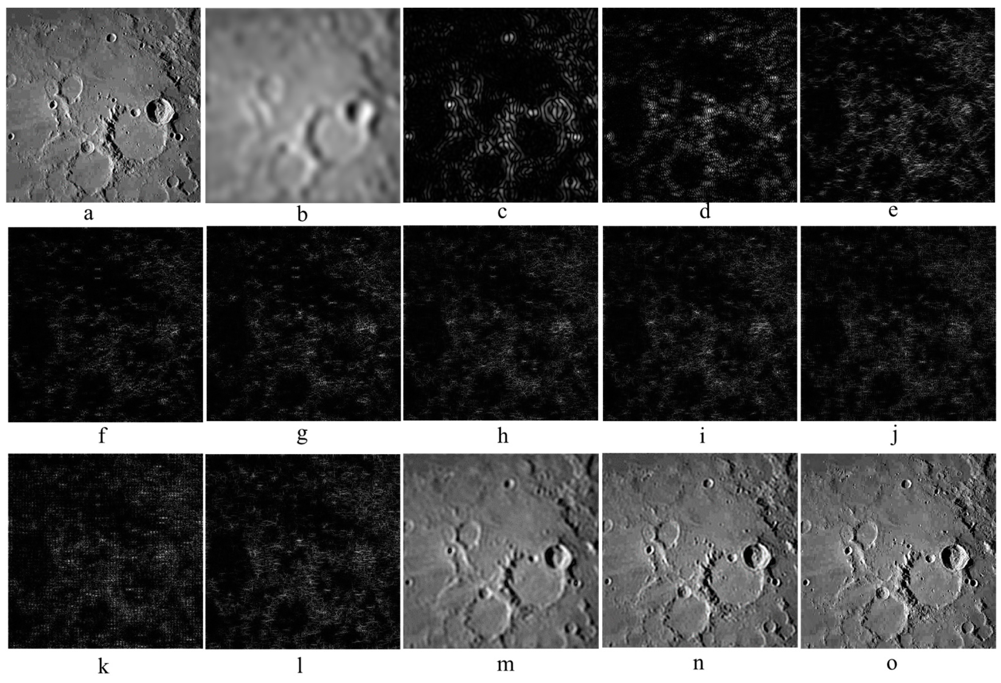
3.3. Examples of Image Analysis with Described 2D Circular Filter Banks

An image analysis is carried out using the 2D circular uniform filter banks of Example 1.

In a, a grayscale picture (from Japan’s lunar lander 2024) with a size of 512 $\times$ 512 pixels representing the Moon’s surface Figure 12a is decomposed with one low-pass filter Figure 12b, nine band-pass filters Figure 12c–k, and one high-pass circular filter Figure 12l.

Figure 12m is produced as a sum of the first two banks: low-pass Figure 12b and band-pass Figure 12c. Figure 12n is produced as a sum of the first three banks: low-pass Figure 12b and band-pass Figure 12c,d. It is seen that Figure 12n depicts the main details. Figure 12o is obtained by summing the outputs of all filters of bank Figure 12b–l and represents the recovered original picture, Figure 12a. The difference between Figure 12a,o is barely noticeable.

Filtration is performed in the frequency domain by multiplying the image spectrum with the filter magnitude response and then applying Inverse Fourier Transform (IFT) to obtain the filtered output image. The filter size is determined by the number of pixels in the image. If the image size is m × n pixels, image processing requires m × n multiplications. Furthermore, processing includes the multiplication of the complex with real numbers and the calculation of the absolute values.

To reduce the computational complexity, it is appropriate to determine the indexes and the values of the non-zero coefficients of the filter bank. For example, for the applied low-pass filter bank in Figure 12b with a size of 512 × 512 = 262,144, the non-zero coefficient is 34,293 or 13.0817%.

The procedure is as follows: the elements of a 512 × 512 zero matrix are replaced with the product of the non-zero coefficients and the values of the image spectrum with their corresponding indexes. Next, we perform IFT.

For the other 10 filter banks, the non-zero coefficients constitute 20.2556%, 28.6652%, 37.1521%, 45.5994%, 54.0558%, 62.3863%, 64.0724%, 60.3218, 52.404%, and 40.6822%, respectively. It should be noted that these percentages also include very small values of non-zero coefficients on the order of 10⁻³²⁴. If a minimum value threshold is set such that any value below that threshold is accepted as zero, those percentages become even lower.

For example, if the minimum value threshold is set to 10⁻⁶ (−100 dB), the percentages of the non-zero coefficients (from the first N = 1 to the last N = 11 filter bank) are as follows: 0.6977%; 2.9602%; 5.9234%; 8.8684%; 11.8225%; 14.7964%; 17.7368; 20.6939%; 23.6481%; 26.6174%; 23.9662%.

An image analysis is performed using the 2D circular nonuniform filter banks of Example 4.

Figure 13a presents a grayscale picture Figure 13a (from Petya Tasheva) with a size of 2048 $\times$ 1152 pixels of a tree branch with the sea and clouds in the background. The picture is decomposed using the six nonlinear filter banks from Example 4: one LP bank Figure 13b, four BP banks Figure 13c–f, and one HP bank Figure 13g. Image processing is performed with the same rules described in the previous example.

Figure 13h is the recovered original picture Figure 13a obtained by summing all filter banks. As in the previous analysis example, the difference is barely noticeable.

4. Discussion and Conclusions

With the sigmoidal function, erfc(.), using the parameter β (2), a 2D band-pass filter with extremely high selectivity and an exact shape can be designed, as shown in Figure 3 and Figure 4. The obtained magnitude response is maximally flat in the passband, smooth in the transition band, and without oscillations in the stopband.

The magnitude response can be defined exactly with arbitrary selectivity.

The filter coefficients are determined by equations, which facilitate the design. There are no approximations, optimizations, iterative algorithms, convergences, etc. For example, the coefficients of the 2D BP filter depicted in Figure 3 for 0.03 s is calculated using MATLAB (version R2023a) and the following notebook: DESKTOP-TK312MM Processor Intel(R) Core(TM) i7-7500U CPU @ 2.70 GHz 2.90 GHz, RAM—12.0 GB.

One of the most important parameters for the comparison of two-dimensional digital filters and filter banks is the computational complexity of the image analysis and the synthesis of the filter itself, i.e., the filter coefficients. In the previous section, it was shown that the significant coefficients of the filter are non-zero, which reduces the number of computational operations.

In general, filter synthesis using erfc(.) is faster than the Parks–McLellan (Remez) algorithm. In [35], a comparison for the case of a 1D FIR filter is described. In the example presented in [35], the total performance time is more than 17 times shorter. This consideration can be extrapolated for 2D filters, because in the 2D case, the number of coefficients is far greater. This can be verified with the following example.

We compare two 2D band pass circular filters with dimensions of 64 × 64 designed with the sigmoidal function efrc(.) and the Remez algorithm. In Figure 14 and Figure 15, the total computational time for both cases is shown.

The total time for the 2D filter synthesis with erfc(.) is 0.004 s, as shown in Figure 14.

The total time for the same 2D filter synthesis with the MATLAB function ftrans2(.), that uses Remez’ algorithm is 0.417 s—Figure 15.

In the figure, it is seen that the Remez algorithm is called 442 times, while the coefficients of the erfc(.) 2D filter are calculated from Equations (5)–(8).

The comparison shows that the proposed 2D filter bank synthesis with erfc(.) is much faster. In the considered case, it is 103.5 times faster.

The filter coefficient calculations can be significantly reduced when the filter’s body is symmetric with respect to the variables f_x and f_y. Such an approach is frequently used in engineering design, electromagnetic simulations, etc.

The 2D uniform and nonuniform filter banks are exactly overlapped at the level of 3.01 dB. The overlap region can be changed using the parameter β.

With the described theory, 2D filter banks with different shapes can be synthesized (18)–(21). The proposed theory is demonstrated by two image analysis examples. The described method complements the 2D filter bank theory.

References

1. Lim, J.S.; Antoniou, A. Two-Dimensional Signal and Image Processing; Prentice Hall: Upper Saddle River, NJ, USA, 1990. [Google Scholar]
2. Lu, W.; Antoniou, A. Two-Dimensional Digital Filters; CRC Press: Boca Raton, FL, USA, 1992. [Google Scholar]
3. Lin, Y.P.; Vaidyanathan, P.P. Theory and design of two-dimensional filter banks: A review. Multidim. Syst. Signal Process. 1996, 7, 263–330. [Google Scholar] [CrossRef]
4. Kumar, S.; Singh, R. A comprehensive review and analysis on digital filter design. Int. J. Adv. Res. Eng. Technol. (IJARET) 2021, 12, 1131–1149. [Google Scholar]
5. Kockanat, D.S.; Karaboga, N. The Design Approaches of Two-Dimensional Digital Filters Based on Metaheuristic Optimization Algorithms: A Review of the Literature; Springer Science+Business Media Dordrecht: Dordrecht, The Nederland, 2015; pp. 265–287. [Google Scholar]
6. Shyu, J.-J.; Pei, S.-C.; Huang, Y.-D. Design of variable two-dimensional FIR digital filters by McClellan transformation. IEEE Trans. Circuits Syst. I Regul. Pap. 2009, 56, 574–582. [Google Scholar] [CrossRef]
7. Wang, Y.; Yue, J.; Su, Y.; Liu, H. Design of two-dimensional zero-phase fir digital filter by McClellan transformation and interval global optimization. IEEE Trans. Circuits Syst. II Express Briefs 2013, 60, 167–171. [Google Scholar] [CrossRef]
8. Rusu, C.; Dumitrescu, B. Iterative reweighted l1 design of sparse FIR filters. Signal Process. 2012, 92, 905–911. [Google Scholar] [CrossRef]
9. Dumitrescu, B. Trigonometric polynomials positive on frequency domains and applications to 2-D FIR filter design. IEEE Trans. Signal Process. 2006, 54, 4282–4292. [Google Scholar] [CrossRef]
10. Hong, X.Y.; Lai, X.P.; Zhao, R.J. Matrixbased algorithms for constrained least-squares and minimax designs of 2-D FIR filters. IEEE Trans. Signal Process. 2013, 64, 3620–3631. [Google Scholar] [CrossRef]
11. Wang, H.; Li, X.; Jhaveri, R.H.; Gadekallu, T.R.; Zhu, M.; Ahanger, T.A.; Khowaja, S.A. Sparse Bayesian learning based channel estimation in FBMC/OQAM industrial IoT networks. Comput. Commun. 2021, 176, 40–45. [Google Scholar] [CrossRef]
12. Kyurkchiev, N.; Zaevski, T.; Iliev, A.; Kyurkchiev, V.; Rahnev, A. Modeling of Some Classes of Extended Oscillators: Simulations, Algorithms, Generating Chaos, and Open Problems. Algorithms 2024, 17, 121. [Google Scholar] [CrossRef]
13. Wang, H.; Xu, L.; Yan, Z.; Gulliver, T.A. Low-Complexity MIMO-FBMC Sparse Channel Parameter Estimation for Industrial Big Data Communications. IEEE Trans. Ind. Inform. 2021, 17, 3422–3430. [Google Scholar] [CrossRef]
14. Bindima, T.; Elias, E. Design and implementation of low complexity 2-D variable digital FIR filters using single-parameter-tunable 2-D Farrow structure. IEEE Trans. Circuits Syst. I Regul. Pap. 2018, 65, 618–627. [Google Scholar] [CrossRef]
15. Matei, R. Efficient design procedure for circular filter banks. In Proceedings of the IEEE 63rd International Midwest Symposium on Circuits and Systems (MWSCAS), East Lansing, MI, USA, 9–11 August 2021; pp. 259–262. [Google Scholar] [CrossRef]
16. Weiping, Z.; Nakamura, S. An efficient approach for the synthesis of 2-D recursive fan filters using 1-D prototypes. IEEE Trans. Signal Process. 1996, 44, 979–983. [Google Scholar] [CrossRef]
17. Bindima, T.; Manuel, M.; Elias, E. An efficient transformation for two dimensional circularly symmetric wideband FIR filters. In Proceedings of the IEEE Region 10 Conference (TENCON), Singapore, 22–25 November 2016; pp. 2838–2841. [Google Scholar] [CrossRef]
18. Hung, T.Q.; Tuan, H.D.; Nguyen, T.Q. Design of half-band diamond and fan filters by SDP. In Proceedings of the IEEE International Conference on Acoustics, Speech and Signal Processing, Honolulu, HI, USA, 15–20 April 2007; Volume III, pp. 901–904. [Google Scholar]
19. Matei, R. A class of directional zero-phase 2D filters designed using analytical approach. IEEE Trans. Circuits Syst. I Regul. Pap. 2022, 69, 1629–1640. [Google Scholar] [CrossRef]
20. Bamberger, R.H.; Smith, M.J.T. A filter bank for the directional decomposition of images: Theory and design. IEEE Trans. Signal Process. 1992, 40, 882–893. [Google Scholar] [CrossRef]
21. Tirakis, A.; Delopoulos, A.; Kollias, S. Two-dimensional filter bank design for optimal reconstruction using limited subband information. IEEE Trans. Image Process. 1995, 4, 1160–1165. [Google Scholar] [CrossRef]
22. Shi, G.; Liang, L.; Xie, X. Design of directional filter banks with arbitrary number of subbands. IEEE Trans. Signal Process. 2009, 57, 4936–4941. [Google Scholar] [CrossRef]
23. Tanaka, Y.; Ikehara, M.; Nguyen, T.Q. A new combination of 1D and 2D filter banks for effective multiresolution image representation. In Proceedings of the 2008 15th IEEE International Conference on Image Processing, San Diego, CA, USA, 12–15 October 2008; pp. 2820–2823. [Google Scholar] [CrossRef]
24. Basu, S. Multidimensional causal, stable, perfect reconstruction filter banks. IEEE Trans. Circuits Syst. I Fundam. Theory Appl. 2002, 49, 832–842. [Google Scholar] [CrossRef]
25. Liang, L.; Shi, G.; Xie, X. Nonuniform directional filter banks with arbitrary frequency partitioning. IEEE Trans. Image Process. 2011, 20, 283–288. [Google Scholar] [CrossRef] [PubMed]
26. Nguyen, T.T.; Oraintara, S. A class of multiresolution directional filter banks. IEEE Trans. Signal Process. 2007, 55, 949–961. [Google Scholar] [CrossRef]
27. Lu, Y.M.; Do, M.N. Multidimensional directional filter banks and surfacelets. IEEE Trans. Image Process. 2007, 16, 918–931. [Google Scholar] [CrossRef]
28. Hendre, M.; Patil, S.; Abhyankar, A. Directional filter bank-based fingerprint image quality. Pattern Anal. Appl. 2022, 25, 379–393. [Google Scholar] [CrossRef]
29. Li, M.; Zhao, Y.; Zhang, F.; Luo, B.; Yang, C.; Gui, W.; Chang, K. Multi-scale feature selection network for lightweight image super-resolution. Neural Netw. 2024, 169, 352–364. [Google Scholar] [CrossRef] [PubMed]
30. Matei, R.; Chiper, D.F. Analytic design technique for 2D FIR circular filter banks and their efficient implementation using polyphase approach. Sensors 2023, 23, 9851. [Google Scholar] [CrossRef] [PubMed]
31. Qobbi, H.; Zoulagh, T.; Barbosa, K.A.; Boukili, B.; Hmamed, A.; Chaibi, N. H∞ filtering of 2D linear FM II model delayed systems. In Proceedings of the ICEGC’2023, Proceedings of the E3S Web of Conferences, Blagoveschensk, Russia, 22–25 May 2023; Volume 469, pp. 1–10. [Google Scholar] [CrossRef]
32. Apostolov, P.S.; Yurukov, B.P.; Stefanov, A.K. An easy and efficient method for synthesizing two-dimensional finite impulse response filters with improved selectivity [Tips & Tricks]. IEEE Signal Process. Mag. 2017, 34, 180–183. [Google Scholar] [CrossRef]
33. Apostolov, P.; Stefanov, A.; Nedialkov, I. Efficient two dimensional filter synthesis. In Proceedings of the 2018 26th Telecommunications Forum (TELFOR), Belgrade, Serbia, 20–21 November 2018; pp. 1–4. [Google Scholar] [CrossRef]
34. Apostolov, P.; Stefanov, A.; Apostolov, S. A study of filters selectivity with maximally flat responses with respect to Harsdorff distance. In Proceedings of the 2018 IX National Conference with International Participation (ELECTRONICA), Sofia, Bulgaria, 17–18 May 2018; pp. 1–3. [Google Scholar] [CrossRef]
35. Apostolov, P.S.; Stefanov, A.K.; Bagasheva, M.S. Efficient FIR filter synthesis using sigmoidal function. In Proceedings of the 2019 X National Conference with International Participation (ELECTRONICA), Sofia, Bulgaria, 16–17 May 2019; pp. 1–4. [Google Scholar] [CrossRef]
36. Apostolov, P.; Meklyov, A.; Kostov, V. Band-pass and band-stop filters synthesis using sigmoidal function. In Proceedings of the 2021 12th National Conference with International Participation (ELECTRONICA), Sofia, Bulgaria, 27–28 May 2021; pp. 1–3. [Google Scholar] [CrossRef]
Figure 1. Magnitude responses of the ideal low-pass filter and the magnitude response of the low-pass filter with the erfc(.).
Electronics 13 04146 g001
Figure 2. Magnitude response of BP filter.
Electronics 13 04146 g002
Figure 3. A 2D band-pass circular filter response in dB with the following parameters: ft = 0.5, β = 385.3394, BW = 0.1, δ = −3.01 dB, and Δf = 1/1000.
Electronics 13 04146 g003
Figure 4. Two-dimensional band-pass circular filter response in dB—top view.
Electronics 13 04146 g004
Figure 5. Two-dimensional circular filter banks: N = 11, β = 38.53393, BW = 0.1, δ = 1 / 2 , and Δf = 0.01.
Electronics 13 04146 g005
Figure 6. Diametral cut of 2D circular filter banks: fx   [−1, 1]; fy = 0.
Electronics 13 04146 g006
Figure 7. Two-dimensional fan filter banks: N = 11, β = 38.53393, BW = 0.1, δ = 1 / 2 , and Δf = 0.01.
Electronics 13 04146 g007
Figure 8. Two-dimensional axial fan filter banks: N = 11, α = π/11, β = 38.53393, δ = 1 / 2 , and Δf = 0.01.
Electronics 13 04146 g008
Figure 9. Two-dimensional axial fan filter bank: N = 1, α = π/11, β = 38.53393, δ = 1 / 2 , θ = 0, and Δf = 0.01.
Electronics 13 04146 g009
Figure 10. The magnitude response of the 2D nonuniform filter banks; N = 6.
Electronics 13 04146 g010
Figure 11. Diametral cut of 2D nonuniform filter banks; N = 6, fx   [−1, 1], fy = 0.
Electronics 13 04146 g011
Figure 12. Image analysis with 2D circular uniform filter banks; N = 11: (a) original image “Moon’s surface”; (b) low-pass filtered; (ck) band-pass filtered with nine uniform BP filter banks; (l) high-pass filtered; (m) recovered image by summing the first two filter banks (b,c); (n) recovered image by summing the first three filter banks (bd); (o) recovered image by summing the outputs of all filter banks (bl).
Electronics 13 04146 g012
Figure 13. Image analysis using 2D circular nonuniform filter banks; N = 6. (a) original image; (b) low-pass filtered; (cf) band-pass filtered with four nonuniform BP filter banks; (g) high-pass filtered; (h) recovered image by summing the outputs of all filter banks (bg).
Electronics 13 04146 g013
Figure 14. Total computational time of 2D band pass circular filter synthesis with erfc(.).
Electronics 13 04146 g014
Figure 15. Total computational time of 2D band pass circular filter synthesis with Remez algorithm.
Electronics 13 04146 g015
Disclaimer/Publisher’s Note: The statements, opinions and data contained in all publications are solely those of the individual author(s) and contributor(s) and not of MDPI and/or the editor(s). MDPI and/or the editor(s) disclaim responsibility for any injury to people or property resulting from any ideas, methods, instructions or products referred to in the content.