Abstract
Unlike the precise methods implemented in constrained programming environments, the proposed approach to preventive planning of Product-as-a-Service offers implements a competitive solution based on Genetic Population Stepping Crawl Threads (GPSCT).GPSCT techniques are used to determine the so-called stepping crawl threads (SCT) that recreate, in subsequent steps, variants of the allocation of sets of leased devices with parameters that meet the expectations of the customers ordering them by means of genetic algorithms. SCTs initiated at a selected point of the Cartesian product space of the functional repertoire of the equipment offered penetrate it in search of offer variants that meet the constraints imposed by the size of the budget and the risk level (i.e., expressed as the likelihood of damaging the device or losing part of its functionality) of individual customers. Two approaches of implementation techniques were used to determine the initial SCT population for the genetic algorithm—branch and bound (BBA) and linear programming (LPA). Many experiments assessed their impact on the computation time and the quality of the obtained solution. The performed computational experiments indicate that the effectiveness of both approaches depends on the specificity of the problem considered each time. Interestingly, for different instances of the problem, an alternative solution can always be selected that is competitive with the exact methods, allowing for a 10-fold increase in scalability.
1. Introduction
The integration of Product-as-a-Service (PaaS) models in contemporary business landscapes has reshaped the traditional paradigms of product delivery, emphasizing the importance of service-oriented approaches [1,2]. However, this shift from traditional product-centric transactions to comprehensive service-based solutions introduces a set of unique challenges, particularly regarding the potential risks to which customers are exposed in situations that threaten to lose some of the functionality of leased devices when accepting equipment providers’ PaaS offers. In the context of PaaS offers, effective resource allocation becomes a crucial aspect of preventive planning to ensure the seamless provision of services while proactively mitigating potential risks [3,4].
The dynamic and evolving nature of PaaS offerings, particularly in preventive planning scenarios, demands a strategic allocation of resources to address uncertainties and preemptively handle potential challenges [3,5]. Conducted research confirms these possibilities. A developed provider–customer reference model [6,7] allows for a formal recognition of the relationships connecting the capabilities of the equipment provider with the needs and limitations of the customer. The scale of the resource allocation problems formulated therein (i.e., the allocation of customized equipment to the customers ordering it) was limited by the capabilities of the available constraints programming environments implementing the adopted declarative representation of the reference model. In the case considered, the number of offers was ≤13, and the number of leased equipment was ≤8.
Although constraint programming can be used to model and optimize resource allocation decisions [8] while adhering to various constraints, e.g., including budget constraints, resource availability, and specific requirements associated with PaaS services, its main deficiency results from high computational costs, especially in the case of a large number of variables and constraints [9,10]. This means it is necessary to combine constraint programming with other optimization and heuristic methods, e.g., genetic algorithms (GA) to enhance its effectiveness in real-world applications.
Unlike the conventional formulation [11,12,13], which searches for a PaaS offer allocation to potential customers, the proposed model looks for the structures of the so-called stepping crawl threads (SCT) reconstructing variants of ordered equipment. SCT stages, which step by step determine new variants of sets of ordered equipment, explore the Cartesian product space of the equipment’s functionalities. Initiated from the starting point, SCTs follow a search for offer variants within the budget and risk constraints of individual customers. Reconstructions of equipment sets ordered by customers are assessed in subsequent SCT states while approximating planned offers.
The adopted model allows the formulation of two types of resource allocation problems. The first one seeks the answer to the question: can all customers be satisfied with the offers they expect without exceeding the PaaS provider’s capabilities? The second one is: how many resources the PaaS provider should have to guarantee offers that satisfy customer expectations? Further considerations will focus on the first of them.
The proposed approach uses two algorithms for generating initial populations of SCTs: the branch and bound approach (BBA) and the linear programming approach (LPA). The size of the initial population and the quality of the individuals comprising it affect the time of selecting the offer and its quality (measured by the number of provider resources used to guarantee the given robustness of the offer). The effectiveness of the proposed BB and LP approaches has been verified experimentally.
To summarize, this paper delves into the resource allocation problem within the framework of preventive planning for PaaS offers, aiming to optimize the utilization of resources and enhance the overall robustness of service delivery. Compared to our previous work [7,14] carried out in this area, its main contribution comes down to the development of a new PaaS offer planning method with significantly increased efficiency (i.e., scalability).
The structure of this study is as follows: Section 2 provides a literature review. Section 3 presents the modeling framework behind preventive planning for Product-as-a-Service offerings. Based on the authors’ introduced solution space concept, distinguishing the concepts of the so-called feasible and robust solution spaces, the problem of proactive planning of leasing offers was formulated. Section 4 elaborates on a branch and bound/linear programming-driven genetic algorithm, dedicated to determining acceptable variants of leasing offers. The case study presented in Section 5 summarizes the results of both qualitative and quantitative computer experiments aimed at assessing the scalability of the proposed approach. Conclusions and directions of future research are suggested in Section 6.
2. Literature Review
The considerations pertain to the formulation of strategies for offering multifunctional devices for rental under the Product-as-a-Service (PaaS) model, addressing key aspects such as the allocation of equipment to customers, failure rates of leased devices, and the proactive scheduling of maintenance services. These strategies must also account for constraints related to the supplier’s capabilities and the associated risks faced by customers in scenarios where device functionality may be compromised.
2.1. Product-as-a-Service
PaaS, also known as “Product-service-systems” has been a widely researched topic in academic literature since the 1990s [15,16]. PaaS represents a transformative business model that shifts focus from product ownership to fulfilling customer needs through servitization, where products are offered as services rather than sold outright, focusing on service performance and circular economy principles [17,18], encouraging manufacturers to design products complemented with services such as repair or replacement in subscription systems making products durable, energy-efficient, and easier to remanufacture or recycle, setting a precedent for sustainability. In the PaaS model products are offered in subscription systems with associated services, and since ownership is not transferred to the customer, there is great potential for the circular economy, as the company is responsible for producing a better product.
In the context under consideration, i.e., the so-called Software-Defined Production Systems, it is also worth pointing out the growing importance of other similar concepts such as Manufacturing-as-a-Service (MaaS) and Serviceability. MaaS is a service that delivers manufactured products by connecting its network of suppliers with its customers on a digital platform [19,20]. MaaS helps in the adoption of distributed manufacturing aiming for flexibility, agility, and enhanced customer orientation in manufacturing building mass customization capabilities, thereby enabling production on demand [21]. In turn, serviceability, which refers to the ease and convenience of performing maintenance, such as availability, modularity, standardization, and compatibility of components, supports the expectations mentioned above [22].
However, some research [23,24] has raised concerns about the potential downsides of leasing. They argue that leasing can lead to a reduction in product durability due to possible misuse by the lessee, who may be less careful with the equipment since they do not own it. To mitigate the risk of equipment abuse, it is important to incentivize lessees to take good care of the leased equipment during the lease period. Therefore, an offer type that encourages such responsible behavior, benefiting both parties in the lease agreement, needs to be developed.
In the PaaS model, the lessor typically includes maintenance services as part of the lease agreement [25]. This makes the lessor responsible for implementing an effective maintenance strategy, particularly for preventive maintenance (PVM) and/or predictive maintenance (PDM), to ensure the equipment remains operational in a cost-effective manner.
2.2. Leasing Maintenance Strategies
The literature on the subject distinguishes the following types of maintenance: corrective, preventive, predictive, and normative. Corrective maintenance is performed when a fault is detected or when there are clear signs of a malfunction. Preventive maintenance, on the other hand, is scheduled at specific intervals to prevent potential failures. Predictive maintenance takes this a step further by using time-based data and insights to anticipate and prevent failures, thereby avoiding downtime. Finally, prescriptive maintenance not only predicts potential issues but also provides actionable recommendations on how to control the occurrence of specific events [26,27]. For rented equipment, the most common maintenance strategies are preventive maintenance (PVM) and predictive maintenance (PDM).
The goal of preventive maintenance is to detect and correct any potential problems before they lead to equipment failure, reducing downtime and the need for costly repairs. This type of maintenance aims to move away from corrective maintenance, which is only performed to fix or correct a problem rather than prevent potential issues before they arise. This means that it is usually based on the manufacturer’s recommendations and involves tasks such as inspections, cleaning, lubrication/greasing, tightening, calibration, and parts replacement based on a recurring cycle.
Some scholars have demonstrated that cost-revenue-sharing contracts can ensure supply chain coordination [28]. Various studies have explored such contracts to coordinate the product supply chain among manufacturers, suppliers, retailers, and customers [29,30,31,32], as well as the service supply chain [3,33]. Additionally, a few studies have incorporated warranty contracts into the optimization of PVM policies for leased equipment. For example, Hajej et al. [34] examined the leasing contract during the warranty period, considering its effects on failure rates. Hamidi et al. [35] developed a game-theoretic model where the lessee determined the optimal lease duration and usage rate, while the lessor optimized the PVM policy. Iskandar and Husniah [36], and Iskandar et al. [37], proposed one- and two-dimensional lease contracts with infinite time and usage limits. Wang et al. [38] optimized upgrade and PVM strategies under successive usage-based lease contracts, taking into account the OEM (Original Equipment Manufacturer) warranty, while Husniah et al. [39] considered both crisp and fuzzy usage rates in lease contracts that included service strategies for used products.
In recent years, the application of IoT and other Industry 4.0 technologies has improved maintenance operations. The key idea is to deploy IoT sensors on every machine to facilitate communication between devices, systems, and the flow of information. A network of smart sensors is created to receive real-time data on equipment conditions, which is then analyzed using big data techniques to identify maintenance needs and improve equipment performance and reliability [40,41,42].
Even if proactive and/or predictive maintenance strategies are used, leased equipment failures are also difficult to avoid altogether. Conversely, if no preventive and/or predictive activities are planned, once an unexpected resource failure occurs, any operation on the resource will be rejected during its downtime. To solve this problem, an unplanned maintenance activity is required to restore the equipment to its original state, which always causes longer downtime of the resource, resulting in degraded operations system stability and performance.
To mitigate the impact of such disruptions, a disruption-tolerant planning approach can be integrated into the maintenance strategy. This approach emphasizes the creation of contingency plans and flexible operational workflows that can adapt in real time to equipment failures or resource downtime. By utilizing dynamic scheduling, alternative resource allocation, and real-time monitoring, the system can redirect tasks to other available resources or adjust production schedules to minimize overall downtime. Additionally, predictive analytics can be employed to anticipate potential failures and preemptively adjust operations before a breakdown occurs. This not only reduces the total downtime but also ensures that system performance is maintained at an optimal level, even when unforeseen disruptions arise. By embedding such robustness to disruptions into the planning process, organizations can significantly enhance operational stability and improve their ability to recover from unplanned equipment failures.
2.3. Robustness of Leased Equipment to Loss of Rented Functionalities
Robust planning ensures satisfactory performance across a wide range of future scenarios, while adaptive planning allows for adjustments to unforeseen future conditions [43]. To achieve this, investing in disruption-prevention resources and strategically deploying them after disruptions is essential.
Robustness is a concept that exists in many fields with similar general interpretations, but at a detailed level may be significantly different. Certainly, in cases where robustness is defined by some application-specific metric, the definition has little use outside the application area. However, generally, robustness refers to how a system or plan behaves in the presence of uncertainty. This can, for example, be that some plan is created using estimates of parameters, but operated with a realization of those parameters that can differ from the estimates. A plan that behaves well under a wide range of realizations of parameters is considered robust, whereas a plan that behaves very differently or even fails under different realizations is less robust. In other words, a robust plan is defined as one that delivers outcomes considered satisfactory based on specific assessment criteria across a broad spectrum of plausible future scenarios [44].
As discussed in Section 2.1, planning Platform-as-a-Service (PaaS) offerings under conditions of disruption, such as the failure of leased equipment, has been extensively addressed through various preventive and predictive strategies (see Section 2.2). However, existing approaches in the literature concerning the maintenance of leased devices often fall short of meeting the expectations of both providers and customers. These studies primarily focus on specific aspects of the problem such as maintenance policy for leased equipment [45,46], prognosis and health management (PHM) in the leased manufacturing system [47], warranty for leased equipment from the lessor’s perspective [48], leaving critical gaps unaddressed. To address this limitation, our research extends the classic resource allocation problem (RAP) [49] by incorporating the concept of disruption-robust offers—those that ensure the continuity of expected functionalities even in the event of a device failure. By considering this form of robustness, it becomes possible to mitigate costs associated with the risk of equipment failure.
2.4. Modeling Frameworks
The above-mentioned issues are usually formulated in deterministic models that allow them to be solved by exact operational research methods, such as Mixed-Integer Programming [50] and constraint programming [51], however most often though by approximate methods, including heuristic and metaheuristic methods such as Genetic Algorithms, Adaptive Large Neighborhood Search [52,53], and also deep machine learning [54]. Stochastic representations of scheduling and routing models are rare [55]. A similar situation occurs when trying to model problems described by parameters with uncertain, vague values using the formalism of fuzzy sets and those implementing the declarative modeling paradigm enabling constraint programming environments.
Our previous works [7,14] in the area of planning disruption-robust rental based on a PaaS model dedicated to multifunction devices offers have shown that the concept of robustness can be successfully used in the discussed topic. The research implemented a declarative modeling framework enabling computer experiments in the environment IBM ILOG CPLEX. The results of the conducted studies highlighted the shortcomings of the adopted representation, limiting its use online to relatively small-scale problems. The attempt to overcome these limitations using a Genetic Algorithm (GA) demonstrated its effectiveness [56]. The scale of the problems considered increased by 30%, although at the cost of omitting some feasible solutions. Because GAs are frequently used in optimization problems across industries, concerning areas such as routing, scheduling, and decision-making including PaaS models [57,58,59,60], this direction has been taken up once again in this work. Its aim is to develop a method supporting decision-making enabling the search for a balance between the supply of available equipment (supplier capacity) and customer demand (expectations). Attempts made in this regard concern, for instance, Machine Maintenance Management [61] and Computerized Maintenance Management [62] systems. In addition to these first attempts, it is worth pointing out other research gaps, such as:
- There are no reference models integrating the Product-as-a-Service paradigm with leasing maintenance strategies and techniques ensuring the robustness of leased equipment to the loss of rented functionalities, enabling the search for a balance between the supply of available supplier capacity and customer expectations.
- There is a lack of methods for the integrated preventive-predictive maintenance of multifunctional resources leased to a group of lessors.
- There are no models that allow for taking into account the uncertainty of parameters of leased devices as well as the costs and dates of related services.
Filling these gaps contributes to creating systems supporting both the PaaS provider in planning preventive-predictive maintenance of multifunction devices and its lessors.
3. Preventive Planning of Product-as-a-Service Offers
3.1. The Modeling Framework
The PaaS provider has a set of types of devices: . Each type of device is characterized by a subset of the functionalities from the set (i.e., ). In the algebraic representation, the functionalities of devices can be represented in the form of a matrix . Each row of the matrix (corresponding to the type of device) corresponds to the sequence , where determines whether device type has functionality () or not ():
The number of devices of a given type is determined by the sequence , where means the number of devices of type . The cost of renting each type of device is determined by the sequence , where is the cost of the device type .
There is a set of potential customers looking for offers (sets of devices) that meet their expected assumptions. Each customer expects access to a set of devices that fulfill the functionalities specified by the sequence , where specifies the number of functionalities of type expected by customer . Each customer has a budget , which cannot be exceeded (i.e., the sum of the costs of devices cannot exceed this value).
Each of the potential customers is looking for an offer of PaaS provider devices denoted as the sequence , where means number of type devices offered. The functionalities offered as part of the offer, described with the sequence , can be defined as follows:
where is the number of functionalities made available to customer by the PaaS provider as part of the offer. —product of matrices A and B. For example, if the prepared offer is set according to the sequence: , then customer is offered 1 device of type , 2 devices and 1 device . Assuming that the matrix is: , then (i.e., device type has functionality and ), (i.e., device type has functionality and )) and (i.e., device type has functionality and ). The functionalities offered as part of the offer are therefore described by the sequence (obtained as the product of the matrix —see (2)) of the form: . This means that as part of the presented offer, the customer will have 3 functionalities , 3 functionalities , and 2 functionalities .
The cost of the offer can, in turn, be described by the equation:
In addition to knowing the leasing costs, the customer wants to be sure that in the event of a failure of one or more of the ordered devices, the functionalities of these devices can be met (replaced) by the remaining functional ones. Equipment failure is further understood as a situation in which one of the devices (of type ) fails and its functionalities are no longer available to the customer. As a consequence of this assumption, it becomes possible to introduce the robustness of the offer, understood as the ratio of failure scenarios in which the customer still has the full set of required functionalities () to all considered failure scenarios ():
where means lack of robustness, i.e., for each failure scenario of a single device its functionality cannot be replaced by other functional devices; it means full robustness, i.e., for each failure scenario of a single device, other rented devices offer the functionalities of the malfunction. PaaS provider knows about the robustness level of each customer, therefore his offer must meet the customer’s requirements .
The proposed approach to planning PaaS offerings addresses the main question: Given a set of customers , can a corresponding set of offers be formulated to satisfy their requirements (detailed below)?
To fulfill the specified constraints, each offer must ensure the following:
- (I)
- Functionality: .
- (II)
- Budget: .
- (III)
- Device Availability: .
- (IV)
- Robustness: .
The methodology for identifying offers that satisfy these constraints (I–IV) is outlined in Section 4. This approach is grounded in the “space of stepping crawl thread” concept introduced in Section 3.2
An illustration of an example problem in which a PaaS provider assesses the possibility of preparing robust () offers for two customers ( and ) is shown in Figure 1. The provider has three types of devices respectively in number: fifteen, five, ten. Customers expect offers that include devices that guarantee two functionalities: in numbers eight and five (for customer ) and eleven and three (for customer ), respectively.
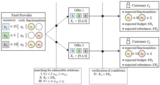
Figure 1.
Planning of Product-as-a-Service offers.
The formulated problem is an extension of the classic problem of resource allocation [63] with the possibility of searching for so-called disruption-robust offers (i.e., guaranteeing the maintenance of expected functionalities in the event of a failure of one of the devices). Taking into account this type of robustness allows you to reduce costs determined by the risk of failure [7].
The problem of searching for disruption-robust offers was first formulated in [6], where constraint programming techniques were used to solve it. Despite many advantages, these techniques are characterized by low computational efficiency. The current scale of problems solvable online is limited to thirteen customers and no more than eight types of devices. The principle of planning offers for a given customer group , which is the basis for the proposed approach, is illustrated in Figure 1.
It assumes that each of the feasible offers is verified in terms of whether it guarantees the expected degree of robustness. It is worth noting that the computational complexity of the problems of determining feasible solutions (constraints No. I–III) and assessing their robustness (constraint No. IV) approximate functions with an exponential course.
3.2. The Solution Space
An algebraic representation of the considered problem (concerning Formulas (1)–(4)) allows the formulation of properties allowing its simplification. Let (—is the number of functionalities of the set ) denote the solution space whose elements are points with coordinates , i.e., . The coordinate of the point determines the number of functionalities made available to the customer as part of the presented offer.
Given is a non-empty set of vectors where and . For example, the set of vectors from the space in Figure 2a) takes the form , where , and
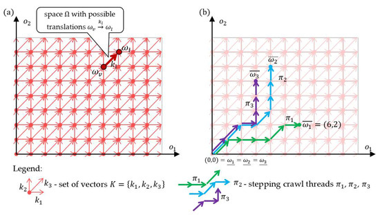
Figure 2.
A two-dimensional structure (a), and examples of the SCTs (b).
The translation of the point by the vector is an operation resulting in the point with coordinates . This type of action is denoted hereafter: . For example, the result of translating the point by the vector is the point i.e., .
The defined space and the operations of translating () the points of this space by the vectors of the set constitute the algebraic structure: , the graphical representation of which (for two dimensions) is shown in Figure 2a). The structure enables to define the concept of a vector path, hereinafter named as stepping crawl thread (SCT). Let the sequence define an SCTs built from the vectors of the set (where , ). The translation of the point by the SCT is the result of successive translations of the point by the vectors making up this path, i.e., . The points and (distinguished by the symbols “_”, “ ”) denote the starting and ending points of the stepping crawl thread , respectively. This translation is further abbreviated as: . An example of 3 vector paths with the origin at point is illustrated in Figure 2b).
In the adopted representation, the elements (edges) of the SCT (with the beginning at the point ) represent the devices constituting the offer made available by the PaaS provider to the customer . However, the coordinates of the endpoint of such a thread determine the functionalities made available under a given offer . The coordinates of the end point of the thread can be determined from the following relationship:
For example, SCT from Figure 2b takes the form: where , . According to (5), the end point is the point representing the functionalities made available to the customer as part of the offer presented by —to the customer who will have 6 functionalities and 2 functionalities .
3.2.1. Subspace of Feasible Solutions
Let us distinguish the subspace containing those solutions that meet the customer’s expectations (i.e., those for which constraint No. I is met—see Section 2.1):
Therefore, each customer corresponds to a set of points that meet his expectations, i.e., points with the coordinates defined by the expression (6). Figure 3 shows examples of spaces (green field) and (blue field) that correspond to the needs of customers from the example shown in Figure 1. Customer expects an offer that guarantees two functionalities ( in the number of eight and five (), respectively, while the customer —in the number eleven and three (). Each point in these spaces defines the conditions that an offer acceptable to customers should meet.
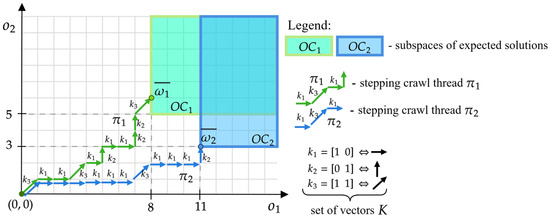
Figure 3.
Spaces of solutions from Figure 1 meeting the expectations of customers , .
In the presented approach, the problem of offer planning comes down to determining a set of the SCTs: , ending at points in the space, i.e., , , …, . Example threads: , , corresponding to the following offers, are shown in Figure 3:
- which consists of: five devices of type , three devices , and three devices ,
- , which consists of: nine devices of type , one device , and two devices .
Of course, not every point of the space can be reached. The number of vectors of the set from which threads are generated is finite (determined by ). The subspace of achievable solutions therefore contains those points that are reachable by the thread generated from the vectors of the set (i.e., points for which constraint No. III is met—see Section 2.1):
where —a function that returns the number of occurrences of the vector in the sequence .
Figure 4 shows the space for the example from Figure 1. Each point of this space represents an offer whose number of shared devices does not exceed the number of devices at the provider’s disposal: , , .
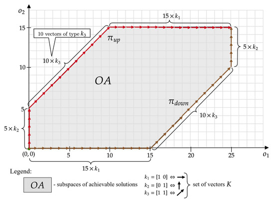
Figure 4.
The space of achievable solutions for , , and .
It is easy to notice that this space is bounded by two threads: , generated from all devices available from the provider:
- ,
- .
We can then define the space of feasible solutions, being the intersection of the space of achievable solutions and the space containing points meeting the customer’s expectations:
A corresponding example of space (green field) and (violet field) that correspond to the feasible solutions for customers from the example shown in Figure 1 is presented in Figure 5.
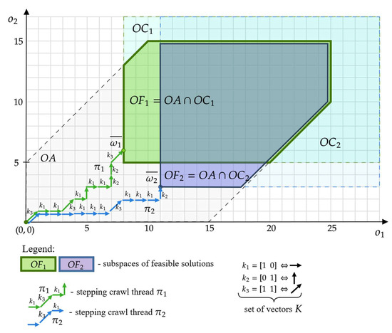
Figure 5.
Spaces of feasible solutions, for example, from Figure 1.
3.2.2. Subspace of Robust Solutions
Of course, searching for threads requires continuous verification of other constraints concerning the offer costs (constraint No. II) and assessment of the offer’s robustness (constraint No. IV). Of the above, the stage of assessing the offer’s robustness is the most computationally expensive. According to (4), this assessment requires an overview of all possible failure scenarios (), the number of which, in general, increases exponentially.
The step of verifying the offer’s robustness assessment (carried out during the construction of the thread) can be removed by introducing a concept of the robust solution space . The robust solution space contains those points of the space which, in the event of a failure (malfunction of any device from the offer), still meet the expectations of the customer . In general, failure of multiple devices can be considered. The failure of devices of type for the offer represented by the thread ending at point can be interpreted as translations of this point by the vector i.e., . If after such a translation the point is located in the area of feasible solutions (i.e., ), then the offer is robust to a given failure scenario. Formally, the space can be defined as follows:
Considered robust solution space contains those points , reaching which (by thread representing the offer ) guarantees full robustness ) of offer . Examples of the robust solution space (the solution space robust to the failure of one device ) and (the space of solutions robust to the failure of two devices ) are illustrated in Figure 6.
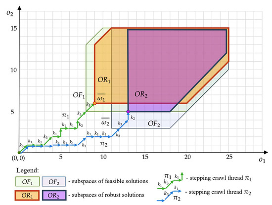
Figure 6.
Spaces , containing robust solutions: .
Each point belonging to these spaces corresponds to offers that meet the expectations of customers and even in the event of failure of a given number of devices (i.e., one device in the case of customer ’s offers, two devices in the case of customer ’s offer). In other words, the spaces , contain points reaching which guarantee full robustness of offers: . An example of threads leading to such points is shown in Figure 6:
- , and
- .
These threads correspond to offers and which guarantee the fulfillment of the functionalities expected by customers: , even in the event of a failure of one (customer ) or two (customer ) of the offered devices.
To sum up, in the space we can distinguish the following subspaces (see Figure 7):
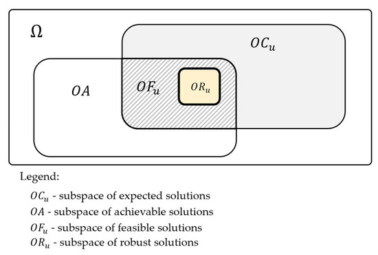
Figure 7.
Structure of subspaces making up the space.
- subspace of expected solutions (6),
- subspace of achievable solutions (7),
- subspace of feasible solutions which is the intersection of and (8),
- subspace of robust solutions which is included in the subspace (9),
3.2.3. Problem Statement
Consequently, the thread obtained in the presented way guarantees robustness . It is worth noting that the introduced representation allows replacing the process of searching for threads that require additional verification of the robustness of the presented offers by the process of searching in for threads that guarantee specific reliability (in the case under consideration, ). Referring to the approach presented in Figure 1, this means that the robust verification stage (verification of constraint No. IV) has been removed from the process of searching for offers. In that context in proposed approach, the considered problem comes down to the following question: Is it possible in the space to determine the SCTs leading to points guaranteeing a given level of robustness (, …, )?
It is worth adding that the points corresponding to solutions with robustness are contained in the space (see an example in Figure 2b). Determining offers that guarantee this type of robustness also comes down to determining the SCTs leading to the points of the space (see the next Section).
4. Genetic Algorithm Driven Approach
The distinguishing feature of the developed genetic algorithm, whose structure corresponds to the conventionally accepted schemes [64,65], is the chromosome defined below.
Let denote the set of feasible solutions (i.e., SCTs) for customer obtained when the expectations of other customers (set ) are ignored. In other words, when constructing the customer offer, the availability of all PaaS provider resources is assumed. The elements of the set are determined using an algorithm based on the branch and bound method or a newly introduced linear programming method, both of which are explained in further subsections.
Chromosome has the form of a sequence of natural numbers where and denotes the number of solutions allowed for customer . The value of specifies the index of solution that was selected for customer from the set . Chromosome thus determines a set of offers (selected from the previously determined sets of feasible solutions ) for all customers of set An example of chromosome is shown in Figure 8.
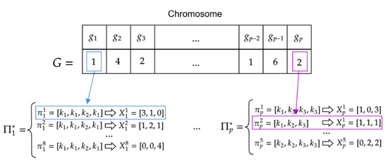
Figure 8.
Example chromosome structure .
The value means that the first possible solution of the form: was adopted for customer (the set contains 8 feasible solutions: ). Similarly, means that the second possible solution of the form: was adopted for customer .
Objective function. It is required that the set of offers defined by the chromosome meets the limitations resulting from the finite number of devices at the PaaS provider’s disposal. Thus, the total number of devices of a given type cannot exceed the value determined by the sequence (where means the number of devices of type ). This constraint is expressed by the following objective function:
where determines the number of devices of type offered as part of the offer determined by the solution . For example, the thread: from Figure 4, determines the offer of the form (3 devices of type : ; 1 device of type : ; 0 devices of type : ).
The objective function defined in this way determines the number of excessive devices in the solution represented by the chromosome.
The developed algorithm searches for the minimum (equal to 0) value of the objective function Determining a chromosome that guarantees such a value means that the offer does not exceed the number of devices at the PaaS provider’s disposal ( sequence). The developed algorithm has the following form (Algorithm 1):
| Algorithm 1. PaaS-Offers-Genetic-Planning |
|
The structure of the algorithm emphasizes, among others: stages of crossbreeding and mutation of population individuals, and, above all, the most important stage of generating the initial population . Two interchangeable ways of determining the population are presented in the Section below.
4.1. Generation of Initial Population
The effectiveness of the developed algorithm depends on the “quality” (i.e., convergence with the searched solution) of the elements constituting the initial population . It is assumed that the quality of the new elements (individuals) generated in the process of population crossover and mutation is determined by the quality of the initial population. In the adopted representation, the initial population is defined as follows:
where —is the set of feasible threads for customer .
The quality of the newly generated populations depends on the appropriate selection of threads of the set determined in accordance with one of two proposed approaches: Branch and Bound Approach and Linear Programming Approach, described below.
4.1.1. Branch and Bound Approach (BBA)
The proposed approach assumes that the threads of the set are branches of the tree rooted in the space (point (0, …, 0)) built from the vectors of the set . An example of such a tree is shown in Figure 9.
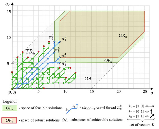
Figure 9.
Example of tree distinguished in space from Figure 5.
The Branch and Bound Approach (BBA) is used to construct a tree , implementing the following principle: a vertex (represented by an appropriate point of the space) can be further expanded (i.e., it may have outgoing edges) if the following conditions are met:
- (a)
- the number of devices available to the supplier has not been exhausted, i.e., .
- (b)
- the customer’s budget has not been exceeded, i.e., .
- (c)
- there are devices that improve the functionality of the offer (represented by branch of tree ), i.e., .
- (d)
- the vertex is not in the space.
A vertex that cannot be expanded according to the above rules becomes a leaf of the tree .
The proposed approach assumes that the set contains threads (branches) of tree (what is hereinafter denoted: —branch is a part of a tree ), which lead to vertices from the space of feasible solutions :
Illustrations of branches belonging to the set (highlighted in blue) on the tree are shown in Figure 9. As you can easily see, all branches end with leaves constituting the vertices of the space. The idea of determining the set by the tree construction is expressed in the following algorithm (Algorithm 2):
| Algorithm 2. Generating feasible solutions, Branch and Bound Approach (BBA) |
|
4.1.2. Linear Programming Approach (LPA)
In this approach, the linear programming method is used to determine the elements of the set (determining the initial population according to (11)). According to the adopted representation, a thread is feasible if the point , to which it leads, belongs to the space: . From the description presented in Section 3, it follows that the space is limited by a convex hyperpolyhedron—see Figure 5.
To simplify the calculations, let us consider a hypercube inscribed in this space i.e., . Figure 10 shows examples of different hypercubes for the space of Figure 5 (taking the shape of squares in two-d space). Each of them corresponds to a different size (length of the edge of the square): , , . In general, the size of hypercube can take the following values: (where is the size of the largest hypercube inscribed in the space).
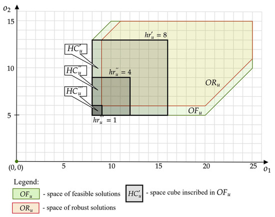
Figure 10.
Example of hypercubes distinguished in space from Figure 5.
In the approach considered, it is assumed that the threads constituting the set are SCTs leading to the space —see Figure 11. Due to the shape of the space taking the form of a hypercube, determining these threads can be represented as solving an appropriate linear programming problem. In this approach, the set takes the form:
where —a function that returns the number of occurrences of the vector in the sequence .
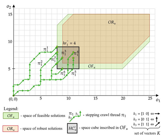
Figure 11.
The set consisting of threads leading to points in the space.
In the proposed approach, inequalities (15)–(17) constitute constraints of the linear model, the solution of which, in the form of variables (for and ) represents a feasible offer of customer . The variables determine the (14) threads leading to the space —as shown in Figure 11.
The advantage of the proposed approach is the ability to reduce the problem of determining feasible threads to a linear programming problem, which can be solved using existing approaches [66,67]. Of course, the set of threads determined in this way is limited only to solutions of the space (of a given size ), which is a subspace of , which means that some of the feasible solutions may be omitted.
The idea of the proposed approach is expressed in the following algorithm (Algorithm 3):
| Algorithm 3. Generating feasible solutions, Linear Programming Approach (LPA) |
|
5. Computational Experiments
The approaches presented in Section 3 and Section 4 were verified on real data collected from a PaaS provider (PP), the description of which, due to its sensitive nature, requires confidentiality. The offered collection distinguishes five types of multifunctional devices (i.e., photocopiers) in various configurations, such as A3 printing, stapling, duplex, and Wi-Fi connectivity. The rental prices of individual types of devices are known, as well as the functionality expectations and budget constraints characterizing the order expectations of each of the twenty customers.
The aim of the experiments is to evaluate alternative approaches to BBA, and LPA described in Section 4.1 and Section 4.1.2, allowing for comparison of generated device rental offers offered by PP to a group of customers with specific capabilities and expectations. An equally important element of this verification is also related to the assessment of time expenditure incurred on solutions in each of these approaches.
5.1. Qualitative Experiments
The experiment used data from PP, which has five types of devices equipped with ten functionalities (see Table 1). PP has the following number of devices of particular types: (in pieces) and the unit rental prices of each of them: (in EURO).

Table 1.
Matrix of functionalities of each device.
The provider considers applications from 20 customers specifying their rental expectations by the number of devices ordered and the types of functionalities provided by them (see Table 2). For example, customer expects that the rented devices will have seven functionalities , four functionalities , seven functionalities , ten functionalities and three functionalities .
Table 2.
Matrix of the customers’ () expectations ().
Each customer has a specific budget and expects a given minimum robustness from the rented equipment (Table 3). For example, customer expects that all rented equipment will cost him at most euros and will have robustness , customer expects that all rented equipment will cost at most euros and will have robustness , etc.
Table 3.
Customers’ () budget and robustness limitations .
The proposed algorithm was run with the following parameters: population size , maximum number of generations , mutation rate . The algorithm was implemented in C++ with the Google OR-Tools library, on an Apple M1 3,2 GHz, 16 GB RAM.
Two solutions were obtained in the form of two alternative offers that meet the requirements of the ordering parties. The first solution (let us call it offer A) presented in Table 4, generated using the BBA algorithm (Seciton 4.1.1), took 173 s to generate, while the alternative (let us call it offer B), see Table 5, was generated using the LPA algorithm (Seciton 4.1.2) in 47 s.
Table 4.
Set of offers for customers obtained by the BBA (offer A).
Table 5.
Set of offers for customers obtained by the LPA (offer B).
In addition to the visible gain in problem-solving time in favor of the LPA algorithm, a difference can be observed in the number of devices assigned to specific customers, which translates into the cost of the offer for the customer/revenue for the provider and the robustness of the ordered equipment.
To sum up, it can be concluded that the relatively small increase in the provider’s revenue provided by offer A (5175 euro compared to 5115 euro obtained in offer B) is not balanced by the loss of robustness (replacement of rented equipment) from the summary level of in offer B to the summary level in offer A. This means that offers obtained using the LPA algorithm are, in general, more favorable for the customer (higher robustness of the rented equipment) at the expense of a slight loss of revenue for the provider.
It is worth adding that in offer A, the provider rents all units of equipment , , and , and is left with only two units of equipment and three units of equipment . In turn, the allocation from offer B results in the rental of all units of equipment and , and seven units of equipment and one unit each of and remain at disposal. This means that the supplier providing offer B will have an additional, larger amount of equipment that could be rented, resulting in additional revenue. This fact once again confirms the competitiveness of the newly developed LPA algorithm.
5.2. Quantitative Experiments
In addition to the qualitative experiments described in Section 5.1, which involve a case study demonstrating the application of the developed model, quantitative experiments were also conducted to evaluate the scale of problems addressed by both proposed approaches.
The problem presented in the previous section constitutes a reference instance (hereinafter referred to as ) for the instances used in the quantitative experiments that follow. Let denote the scale of the problem understood as the proportionality coefficient between the parameters of the generated instance and the reference instance . The parameters subject to scaling are the number of provider devices , the expected functionalities of customers and their budget . It is assumed that the scaled instance is described by the following parameter values (where the superscript () specifies the parameters of the instance and the index () specifies the parameters of the instance):
The remaining parameters of the problem instance remain unchanged.
The experiments were carried out for instances (scale ), the aim of which was to determine offers that meet customer expectations. For this purpose, the developed algorithm in the LPA and BBA variants was used (see Section 4). It is worth noting that the time needed to solve a problem instance is determined by the first stage of the algorithm (generation of an initial population —see Section 4.1), in which sets of feasible solutions (threads ) are determined for each customer. Due to the above, the quantitative experiments conducted focused on the assessment of this stage (i.e., determining the set ).
The experiments distinguished three groups dedicated to answering the following questions:
- At what time is it possible to determine the solution to the problem for the given instances: using both variants of the algorithm: LPA and BBA?
- What is the minimum size of hypercube (LPA algorithm) that guarantees solving a problem of a given scale ?
- What is the time to obtain a solution to the problem with the LPA variant for a given scale s, for different sizes of hypercube ?
The calculations were performed in the environment described in Section 5.1 assuming the population size , maximum number of generations , mutation rate . The developed genetic algorithm was implemented in C++ with the Google OR-Tools library and ran on an Apple M1 3.2 GHz processor, with 16 GB RAM.
Ad. I. The calculation times of generating a solution to the problem in the proposed two approaches were compared. The results for various instances of the scale are presented in Table 6 and Figure 12. For the LPA, two sample values of the size of hypercube were adopted: : and . It is easy to notice that for small scales () the BBA allows solving the problem in a shorter time (even less than a second) compared to the LPA, while for the scale the LPA solves the same problem faster. It is worth noting that the solution time obtained as a result of using the BBA increases very quickly as the scale of the problem increases, while for the LPA the solution time for most of the tested scale values remains at a similar level.
Table 6.
Calculation times of the scale of problem instances for the considered algorithms.
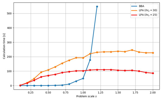
Figure 12.
Time to determine the set of feasible solutions for the following problem scales: .
Ad. II. The significant advantage of the LPA algorithm (especially for “large” scales of problem instances) meant that further experiments focused only on assessing the impact of the parameters of this algorithm. First, the influence of the size value of hypercube on the possibility of obtaining a feasible solution, i.e., was examined. In other words, an attempt was made to assess the minimum size of hypercube for which there is a solution to a problem with scale . The results obtained are illustrated in Figure 13. It can be seen that the minimum value of increases linearly with the scale . It is evident that selecting a value of that is too low for a given scale leads to the absence of an acceptable solution. The experiments conducted indicate that this value should not fall below the trend line represented in the data from Figure 13:
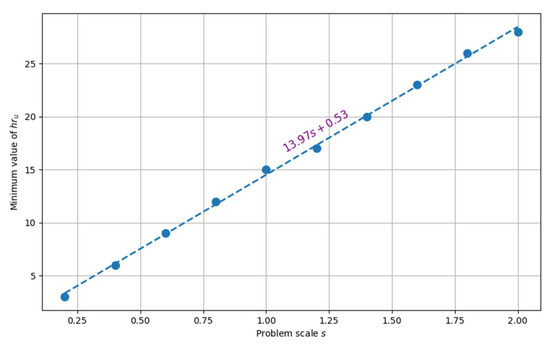
Figure 13.
The minimum value needed to solve the problem at a given scale.
The above relationship determines the lower limit of the parameter, beyond which the LPA algorithm does not return to a feasible solution for the considered instances.
It is worth noting that the possibility of automatically generating the value of this parameter, i.e., selecting it depending on the given scale of the problem, raises a promising topic for future research.
Ad. III. In subsequent experiments, it was checked how the calculation time changes depending on the value of with a constant problem scale . The results emphasizing its non-linear dependence on the hypercube’s size are shown in Figure 14. The observed effect results from the fact that as the value increases, the number of points belonging to hypercube increases exponentially.
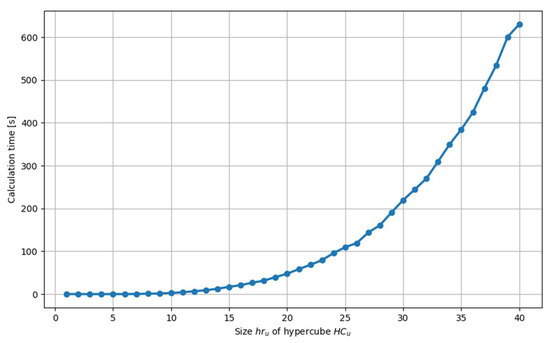
Figure 14.
Time to determine the set of feasible solutions at scale .
The rapid increase in computation time associated with a linear increase in scale significantly constrains the value of . For instance, if we assume that the time required to determine a solution does not exceed 10 min, this condition restricts to values less than 40.
The results of quantitative experiments showed the advantage of the LPA algorithm. For example, for the scale , the time to obtain the response of this algorithm was three times smaller than in the BBA algorithm (see Table 6). However, the effectiveness of the LPA algorithm depends on the appropriate selection of the value—if it is too small, the algorithm will not find feasible solutions. On the other hand, if the parameter value is too large, the time to solve the problem instance will be greater than acceptable, e.g., in online systems.
The resulting scalability of the proposed approach, determined by the minimum value of for a given scale (Figure 13), and the time of determining the set of solutions allowed for a given value of (Figure 14), is illustrated in Figure 15. It can be seen that its implementation in online mode is limited to problems of scale . This means that the presented approach is applicable in situations where the number of devices presented in offers does not exceed 450.
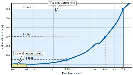
Figure 15.
Scalability of the algorithm implementing LPA—scale of current results are presented in [14,52].
To summarize, previous research [14,52] examining the potential of both declarative programming environments and population algorithms has demonstrated the feasibility of addressing these problems at a scale of (where the number of devices does not exceed 100). In comparison, the approach implemented in the LPA, which operates at a problem scale of (as shown in Figure 15), is more time-efficient than the existing solutions for planning multi-functional equipment leasing offers within the PaaS model.
6. Conclusions
Addressing the issue of preventive planning for PaaS, this work proposes a model enabling the search for resource allocation that meets the risk level expected by the customer while enabling the implementation of dedicated computer-aided supporting decision-making. The developed model implements the authors’ concept of stepping crawl threads, which allows, step by step, to generate variants of allocation of sets of leased devices with parameters that meet the expectations of the customers ordering them.
The case study has demonstrated the practical implementation of the suggested approach in a scenario with twenty customers and five device types with ten functionalities. The findings of this research are applicable in decision support systems for preventive planning of leasing offers while focusing on mitigating customer risks associated with accepting equipment providers’ offers. The scalability of the obtained solution is many times higher than previously obtained results. The proposed approach based on the linear programming method (LPA) allows to increase the scale of previously solved problems (using the BBA method) from 100 to 450 offered devices. That means it provides for taking up challenges posed by problems of a size encountered in practice.
However, high computational efficiency comes at the cost of the obtained solution quality. The obtained solutions often require the PaaS provider to have additional resources (not previously available), even if it is not necessary in reality. Moreover, the developed model does not consider uncertain data related to the fault and servicing of the offered resources. Therefore, future work involves extending the model to include activities related to servicing rented equipment and including cases related to work time uncertainty, while meeting expectations related to minimizing the total cost of maintaining the serviced equipment. Its significant extension should include cases related to the uncertainty of service teams’ working time as well as costs and risks expressed in fuzzy numbers.
The proposed model is distinguished by its open and flexible architecture, which facilitates the seamless incorporation of additional constraints to address the specific requirements of an offer or a particular customer. This adaptability ensures that any extensions or modifications involve merely augmenting the existing set of constraints, without adversely affecting the computational efficiency of the solution. Such a design is particularly advantageous in dynamic and rapidly evolving application contexts, where both PaaS providers and their customers must navigate an environment shaped by shifting operational guidelines, competitive dynamics, and regulatory changes. The model’s inherent flexibility and responsiveness enable it to maintain relevance and effectiveness in the fluid landscape of the leasing industry.
Future research will focus on the development of methodologies for identifying and analyzing factors that influence the balance between supply and demand in PaaS-driven markets. A key area of investigation will center on the provider’s perspective, specifically the trade-offs between the costs associated with equipment procurement by the primary PaaS provider and the expenses incurred for maintenance services outsourced to third-party vendors. By extending the model to capture trade-offs from both supply- and demand-side perspectives, this research aims to provide a comprehensive framework for understanding the dynamic interactions that underpin equilibrium in service-oriented industries, ultimately enhancing the ability to manage and sustain balance within the PaaS market.
Author Contributions
Conceptualization, E.S., G.B. and Z.B.; methodology, K.N. and G.B.; software, K.N.; validation, K.N. and E.S.; formal analysis, G.B. and Z.B.; investigation, E.S. and Z.B.; resources, K.N. and E.S.; data curation, E.S. and K.N.; writing—original draft preparation, Z.B., G.B. and E.S.; writing—review and editing, Z.B. and E.S.; visualization, G.B. and K.N.; supervision, Z.B., E.S. and G.B.; project administration, E.S., Z.B. and G.B. All authors have read and agreed to the published version of the manuscript.
Funding
This research received no external funding.
Data Availability Statement
Data are contained within the article.
Conflicts of Interest
The authors declare no conflicts of interest.
References
- Aas, T.H.; Breunig, K.J.; Hellström, M.M.; Hydle, K.M. Service-Oriented Business Models in Manufacturing in the Digital Era: Toward a New Taxonomy. Int. J. Innov. Manag. 2020, 24, 2040002. [Google Scholar] [CrossRef]
- Kesavapanikkar, P.; Amit, R.K.; Ramu, P. Product as a Service (PaaS) for Traditional Product Companies: An Automotive Lease Practice Evaluation. J. Indian Bus. Res. 2023, 15, 40–54. [Google Scholar] [CrossRef]
- Liu, B.; Wang, Y.; Yang, H.; Segerstedt, A.; Zhang, L. Maintenance Service Strategy for Leased Equipment: Integrating Lessor-Preventive Maintenance and Lessee-Careful Protection Efforts. Comput. Ind. Eng. 2021, 156, 107257. [Google Scholar] [CrossRef]
- Li, K.; Tsou, C.-Y. Leasing as a Risk-Sharing Mechanism. SSRN Electron. J. 2019. [Google Scholar] [CrossRef]
- Hidalgo-Crespo, J.; Riel, A. Towards User-Centric Design Guidelines for PaaS Systems: The Case of Home Appliances; Springer Nature: Cham, Switzerland, 2023; pp. 186–195. [Google Scholar]
- Szwarc, E.; Golińska-Dawson, P.; Bocewicz, G.; Banaszak, Z. Robust Scheduling of Multi-Skilled Workforce Allocation: Job Rotation Approach. Electronics 2024, 13, 392. [Google Scholar] [CrossRef]
- Szwarc, E.; Bocewicz, G.; Smutnicki, C.; Banaszak, Z. Preventive Planning of Product-as-a-Service Offers to Maintain the Availability of Required Service Level. Ann. Oper. Res. 2024, 335, 1–26. [Google Scholar] [CrossRef]
- Sitek, P.; Wikarek, J.; Nielsen, P. A Constraint-Driven Approach to Food Supply Chain Management. Ind. Manag. Data Syst. 2017, 117, 2115–2138. [Google Scholar] [CrossRef]
- Heinz, S.; Ku, W.-Y.; Beck, J.C. Recent Improvements Using Constraint Integer Programming for Resource Allocation and Scheduling. In Proceedings of the Integration of AI and OR Techniques in Constraint Programming for Combinatorial Optimization Problems. CPAIOR 2013, Yorktown Heights, NY, USA, 18–22 May 2013; Lecture Notes in Computer Science. Gomes, C., Sellmann, M., Eds.; Springer: Berlin/Heidelberg, Germany, 2013; Volume 7874, pp. 12–27. [Google Scholar]
- Meng, L.; Zhang, C.; Ren, Y.; Zhang, B.; Lv, C. Mixed-Integer Linear Programming and Constraint Programming Formulations for Solving Distributed Flexible Job Shop Scheduling Problem. Comput. Ind. Eng. 2020, 142, 106347. [Google Scholar] [CrossRef]
- Mustonen, E.; Harkonen, J.; Haapasalo, H. From Product to Service Business: Productization of Product-Oriented, Use-Oriented, and Result-Oriented Business. In Proceedings of the 2019 IEEE International Conference on Industrial Engineering and Engineering Management (IEEM), Macao, Chian, 15–18 December 2019; IEEE: New York, NY, USA, 2019; pp. 985–989. [Google Scholar]
- Octoberry, M.F.; Wittendorp, P. Analyzing of Product as a Service Method in Controlling Production Cost Based on ComPanies in United Kingdom. Diponegoro J. Account. 2023, 12, 1–8. [Google Scholar]
- Sakao, T.; Golinska-Dawson, P.; Vogt Duberg, J.; Sundin, E.; Hidalgo Crespo, J.; Riel, A.; Peeters, J.; Green, A.; Mathieux, F. Product-as-a-Service for Critical Raw Materials: Challenges, Enablers, and Needed Research. In Proceedings of the Going Green: CARE INNOVATION, Vienna, Austria, 8–11 May 2023. [Google Scholar]
- Szwarc, E.; Golińska-Dawson, P.; Bocewicz, G.; Banaszak, Z. Proactive Resource Maintenance in Product-as-a-Service Business Models: A Constraints Programming Based Approach for MFP Offerings Prototyping. In Advances in Manufacturing IV. Volume 2—Production Engineering: Digitalization, Sustainability and Industry Applications; Trojanowska, J., Kujawińska, A., Pavlenko, I., Husar, J., Eds.; Springer: Cham, Switzerland, 2024; pp. 276–289. [Google Scholar]
- Wang, N.; Ren, S.; Liu, Y.; Yang, M.; Wang, J.; Huisingh, D. An Active Preventive Maintenance Approach of Complex Equipment Based on a Novel Product-Service System Operation Mode. J. Clean. Prod. 2020, 277, 123365. [Google Scholar] [CrossRef]
- Xing, K.; Ness, D. Transition to Product-Service Systems: Principles and Business Model. Procedia CIRP 2016, 47, 525–530. [Google Scholar] [CrossRef][Green Version]
- Hidalgo-Crespo, J.; Riel, A.; Duberg, J.V.; Bunodiere, A.; Golinska-Dawson, P. An Exploratory Study for Product-as-a-Service (PaaS) Offers Development for Electrical and Electronic Equipment. Procedia CIRP 2024, 122, 521–526. [Google Scholar] [CrossRef]
- Petänen, P.; Sundqvist, H.; Antikainen, M. Deconstructing Customer Value Propositions for the Circular Product-as-a-Service Business Model: A Case Study from the Textile Industry. Circ. Econ. Sustain. 2024, 4, 1631–1653. [Google Scholar] [CrossRef]
- Bulut, S.; Wende, M.; Wagner, C.; Anderl, R. Impact of Manufacturing-as-a-Service: Business Model Adaption for Enterprises. Procedia CIRP 2021, 104, 1286–1291. [Google Scholar] [CrossRef]
- Chaudhuri, A.; Datta, P.P.; Fernandes, K.J.; Xiong, Y. Optimal Pricing Strategies for Manufacturing-as-a Service Platforms to Ensure Business Sustainability. Int. J. Prod. Econ. 2021, 234, 108065. [Google Scholar] [CrossRef]
- Kohtala, C. Addressing Sustainability in Research on Distributed Production: An Integrated Literature Review. J. Clean. Prod. 2015, 106, 654–668. [Google Scholar] [CrossRef]
- Keller, L.; Maghazei, O.; Gróf, C.; Netland, T.H. Exploring Servitization in Building Technology: The Case of Piping Systems. In Advances in Production Management Systems. Production Management Systems for Volatile, Uncertain, Complex, and Ambiguous Environments; APMS 2024. IFIP Advances in Information and Communication Technology; Thürer, M., Riedel, R., von Cieminski, G., Romero, D., Eds.; Springer: Cham, Switzerland, 2024; Volume 728, pp. 250–261. [Google Scholar]
- Demailly, D.; Novel, A.-S. The Sharing Economy: Make It Sustainable. Studies 2014, 3, 14–30. [Google Scholar]
- Evans, S.; Partidário, P.J.; Lambert, J. Industrialization as a Key Element of Sustainable Product-Service Solutions. Int. J. Prod. Res. 2007, 45, 4225–4246. [Google Scholar] [CrossRef]
- Xia, T.; Dong, Y.; Xiao, L.; Du, S.; Pan, E.; Xi, L. Recent Advances in Prognostics and Health Management for Advanced Manufacturing Paradigms. Reliab. Eng. Syst. Saf. 2018, 178, 255–268. [Google Scholar] [CrossRef]
- Matyas, K.; Nemeth, T.; Kovacs, K.; Glawar, R. A Procedural Approach for Realizing Prescriptive Maintenance Planning in Manufacturing Industries. CIRP Ann. 2017, 66, 461–464. [Google Scholar] [CrossRef]
- Nemeth, T.; Ansari, F.; Sihn, W.; Haslhofer, B.; Schindler, A. PriMa-X: A Reference Model for Realizing Prescriptive Maintenance and Assessing Its Maturity Enhanced by Machine Learning. Procedia CIRP 2018, 72, 1039–1044. [Google Scholar] [CrossRef]
- Cachon, G.P.; Lariviere, M.A. Supply Chain Coordination with Revenue-Sharing Contracts: Strengths and Limitations. Manag. Sci. 2005, 51, 30–44. [Google Scholar] [CrossRef]
- Wu, D.; Chen, J.; Li, P.; Zhang, R. Contract Coordination of Dual Channel Reverse Supply Chain Considering Service Level. J. Clean. Prod. 2020, 260, 121071. [Google Scholar] [CrossRef]
- Liu, Z.; Hua, S.; Zhai, X. Supply Chain Coordination with Risk-Averse Retailer and Option Contract: Supplier-Led vs. Retailer-Led. Int. J. Prod. Econ. 2020, 223, 107518. [Google Scholar] [CrossRef]
- Kunter, M. Coordination via Cost and Revenue Sharing in Manufacturer–Retailer Channels. Eur. J. Oper. Res. 2012, 216, 477–486. [Google Scholar] [CrossRef]
- He, Y.; Zhao, X.; Zhao, L.; He, J. Coordinating a Supply Chain with Effort and Price Dependent Stochastic Demand. Appl. Math. Model. 2009, 33, 2777–2790. [Google Scholar] [CrossRef]
- Qin, X.; Su, Q.; Huang, S.H.; Wiersma, U.J.; Liu, M. Service Quality Coordination Contracts for Online Shopping Service Supply Chain with Competing Service Providers: Integrating Fairness and Individual Rationality. Oper. Res. 2019, 19, 269–296. [Google Scholar] [CrossRef]
- Hajej, Z.; Rezg, N.; ali, G. An Optimal Production/Maintenance Strategy under Lease Contract with Warranty Periods. J. Qual. Maint. Eng. 2016, 22, 35–50. [Google Scholar] [CrossRef]
- Hamidi, M.; Liao, H.; Szidarovszky, F. Non-Cooperative and Cooperative Game-Theoretic Models for Usage-Based Lease Contracts. Eur. J. Oper. Res. 2016, 255, 163–174. [Google Scholar] [CrossRef]
- Iskandar, B.P.; Husniah, H. Optimal Preventive Maintenance for a Two Dimensional Lease Contract. Comput. Ind. Eng. 2017, 113, 693–703. [Google Scholar] [CrossRef]
- Iskandar, B.P.; Wangsaputra, R.; Pasaribu, U.S.; Husniah, H. Optimal Lease Contract for Remanufactured Equipment. IOP Conf. Ser. Mater. Sci. Eng. 2018, 319, 012070. [Google Scholar] [CrossRef]
- Wang, X.; Li, L.; Xie, M. Optimal Preventive Maintenance Strategy for Leased Equipment under Successive Usage-Based Contracts. Int. J. Prod. Res. 2019, 57, 5705–5724. [Google Scholar] [CrossRef]
- Husniah, H.; Supriatna, A.K.; Iskandar, B.P. Lease Contract with Servicing Strategy Model for Used Product Considering Crisp and Fuzzy Usage Rate. Int. J. Artif. Intell. 2018, 18, 177–192. [Google Scholar]
- Lee, J.; Ardakani, H.D.; Yang, S.; Bagheri, B. Industrial Big Data Analytics and Cyber-Physical Systems for Future Maintenance & Service Innovation. Procedia CIRP 2015, 38, 3–7. [Google Scholar] [CrossRef]
- Kan, C.; Yang, H.; Kumara, S. Parallel Computing and Network Analytics for Fast Industrial Internet-of-Things (IIoT) Machine Information Processing and Condition Monitoring. J. Manuf. Syst. 2018, 46, 282–293. [Google Scholar] [CrossRef]
- Cañas, H.; Mula, J.; Campuzano-Bolarín, F. A General Outline of a Sustainable Supply Chain 4.0. Sustainability 2020, 12, 7978. [Google Scholar] [CrossRef]
- Haasnoot, M.; Middelkoop, H.; van Beek, E.; van Deursen, W.P.A. A Method to Develop Sustainable Water Management Strategies for an Uncertain Future. Sustain. Dev. 2011, 19, 369–381. [Google Scholar] [CrossRef]
- Rosehead, J.; Mingers, J. Rational Analysis for a Problematic World Revisted: Problem Structuring Methods for Complexity, Uncertained and Conflict. Syst. Res. Behav. Sci. 2001, 19, 383–385. [Google Scholar]
- Schutz, J.; Rezg, N. Maintenance Strategy for Leased Equipment. Comput. Ind. Eng. 2013, 66, 593–600. [Google Scholar] [CrossRef]
- Liu, B.; Pang, J.; Yang, H.; Zhao, Y. Optimal Condition-Based Maintenance Policy for Leased Equipment Considering Hybrid Preventive Maintenance and Periodic Inspection. Reliab. Eng. Syst. Saf. 2024, 242, 109724. [Google Scholar] [CrossRef]
- Zhang, K.; Xia, T.; Si, G.; Pan, E.; Xi, L. An Edge-Based Framework for Real-Time Prognosis and Opportunistic Maintenance in Leased Manufacturing System. IEEE Trans. Autom. Sci. Eng. 2024, 21, 4177–4187. [Google Scholar] [CrossRef]
- Ben Mabrouk, A.; Chelbi, A. Joint Preventive Maintenance and Extended Warranty Strategy for Leased Unreliable Equipment Submitted to Imperfect Repair at Failure. IFAC-PapersOnLine 2022, 55, 1201–1206. [Google Scholar] [CrossRef]
- Strimovskaya, A.; Barykin, S. A Multidimensional Approach to the Resource Allocation Problem (RAP) through the Prism of Industrial Information Integration (III). J. Ind. Inf. Integr. 2023, 34, 100473. [Google Scholar] [CrossRef]
- Guastaroba, G.; Côté, J.-F.; Coelho, L.C. The Multi-Period Workforce Scheduling and Routing Problem. Omega 2021, 102, 102302. [Google Scholar] [CrossRef]
- Güner, F.; Görür, A.K.; Satır, B.; Kandiller, L.; Drake, J.H. A Constraint Programming Approach to a Real-World Workforce Scheduling Problem for Multi-Manned Assembly Lines with Sequence-Dependent Setup Times. Int. J. Prod. Res. 2024, 62, 3212–3229. [Google Scholar] [CrossRef]
- Ali, O.; Côté, J.-F.; Coelho, L.C. Models and Algorithms for the Delivery and Installation Routing Problem. Eur. J. Oper. Res. 2021, 291, 162–177. [Google Scholar] [CrossRef]
- Pham, D.T.; Kiesmüller, G.P. Hybrid Value Function Approximation for Solving the Technician Routing Problem with Stochastic Repair Requests. Transp. Sci. 2024, 58, 499–519. [Google Scholar] [CrossRef]
- Sharifani, K.; Amini, M. Machine Learning and Deep Learning: A Review of Methods and Applications. World Inf. Technol. Eng. J. 2023, 10, 3897–3904. [Google Scholar]
- Wang, R.; Shehadeh, K.S.; Xie, X.; Li, L. Data-Driven Integrated Home Service Staffing and Capacity Planning: Stochastic Optimization Approaches. Comput. Oper. Res. 2023, 159, 106348. [Google Scholar] [CrossRef]
- Niemiec, K.; Szwarc, E.; Bocewicz, G.; Banaszak, Z. Genetic Algorithm for Preventive Planning of Product-as-a-Service Offers. In Distributed Computing and Artificial Intelligence, Special Sessions I; Springer: Cham, Switzerland, 2024; in print. [Google Scholar]
- Alhamad, K.; Alkhezi, Y. Hybrid Genetic Algorithm and Tabu Search for Solving Preventive Maintenance Scheduling Problem for Cogeneration Plants. Mathematics 2024, 12, 1881. [Google Scholar] [CrossRef]
- Katoch, S.; Chauhan, S.S.; Kumar, V. A Review on Genetic Algorithm: Past, Present, and Future. Multimed. Tools Appl. 2021, 80, 8091–8126. [Google Scholar] [CrossRef] [PubMed]
- Muniasamy, K.; Venugopal, P.; Pakkirisamy, G. Genetic Algorithm-Driven Optimization of Scheduling and Preventive Measures in Parallel Machines. Math. Model. Eng. Probl. 2023, 10, 1811–1816. [Google Scholar] [CrossRef]
- Javanmard, H.; Koraeizadeh, A.a.-W. Optimizing the Preventive Maintenance Scheduling by Genetic Algorithm Based on Cost and Reliability in National Iranian Drilling Company. J. Ind. Eng. Int. 2016, 12, 509–516. [Google Scholar] [CrossRef]
- Asri, A.A.M.; Isa, M.A. A System for Preventive Maintenance: Machine Maintenance Management System. In UTM Computing Proceedings Innovations in Computing Technology and Applications; 2018; Volume 3, ISBN 978-967-2171-30-0. Available online: http://eprints.utm.my/83578/ (accessed on 15 October 2024).
- Kuroki, A.; Cardoso, V.H.; Neto, G.C.O.; Amorim, M. The Implementation of Preventive Maintenance in a Product-Service System (PSS) Business Model. In Flexible Automation and Intelligent Manufacturing: Establishing Bridges for More Sustainable Manufacturing Systems. FAIM 2023. Lecture Notes in Mechanical Engineering; Silva, F.J.G., Ferreira, L.P., Sá, J.C., Pereira, M.T., Pinto, C.M.A., Eds.; Springer: Cham, Switzerland, 2024; pp. 60–68. [Google Scholar]
- Forootani, A.; Tipaldi, M.; Ghaniee Zarch, M.; Liuzza, D.; Glielmo, L. Modelling and Solving Resource Allocation Problems via a Dynamic Programming Approach. Int. J. Control 2021, 94, 1544–1555. [Google Scholar] [CrossRef]
- Sohail, A. Genetic Algorithms in the Fields of Artificial Intelligence and Data Sciences. Ann. Data Sci. 2023, 10, 1007–1018. [Google Scholar] [CrossRef]
- Gen, M. Genetic Algorithms and Their Applications. In Springer Handbook of Engineering Statistics. Springer Handbooks; Springer: London, UK, 2023. [Google Scholar]
- Anh-Dung, N.; Duy-Thai, L. Combining Genetic Algorithms And Or-Tools To Solve Flexible Job-Shop Scheduling Problems. In Proceedings of the 2024 IEEE 11th International Conference on Computational Cybernetics and Cyber-Medical Systems (ICCC), Hanoi, Vietnam, 4–6 April 2024; IEEE: New York, NY, USA, 2024; pp. 000219–000224. [Google Scholar]
- Oliveira, M.; Rocha, A.M.A.C.; Alves, F. Using OR-Tools When Solving the Nurse Scheduling Problem. In Optimization, Learning Algorithms and Applications. OL2A 2023. Communications in Computer and Information Science; Pereira, A.I., Mendes, A., Fernandes, F.P., Pacheco, M.F., Coelho, J.P., Lima, J., Eds.; Springer: Cham, Switzerland, 2024; Volume 1981, pp. 438–449. [Google Scholar]


Disclaimer/Publisher’s Note: The statements, opinions and data contained in all publications are solely those of the individual author(s) and contributor(s) and not of MDPI and/or the editor(s). MDPI and/or the editor(s) disclaim responsibility for any injury to people or property resulting from any ideas, methods, instructions or products referred to in the content. |
© 2024 by the authors. Licensee MDPI, Basel, Switzerland. This article is an open access article distributed under the terms and conditions of the Creative Commons Attribution (CC BY) license (https://creativecommons.org/licenses/by/4.0/).