
High-Quality Instance Mining and Weight Re-Assigning for Weakly Supervised Object Detection in Remote Sensing Images

Abstract
1. Introduction
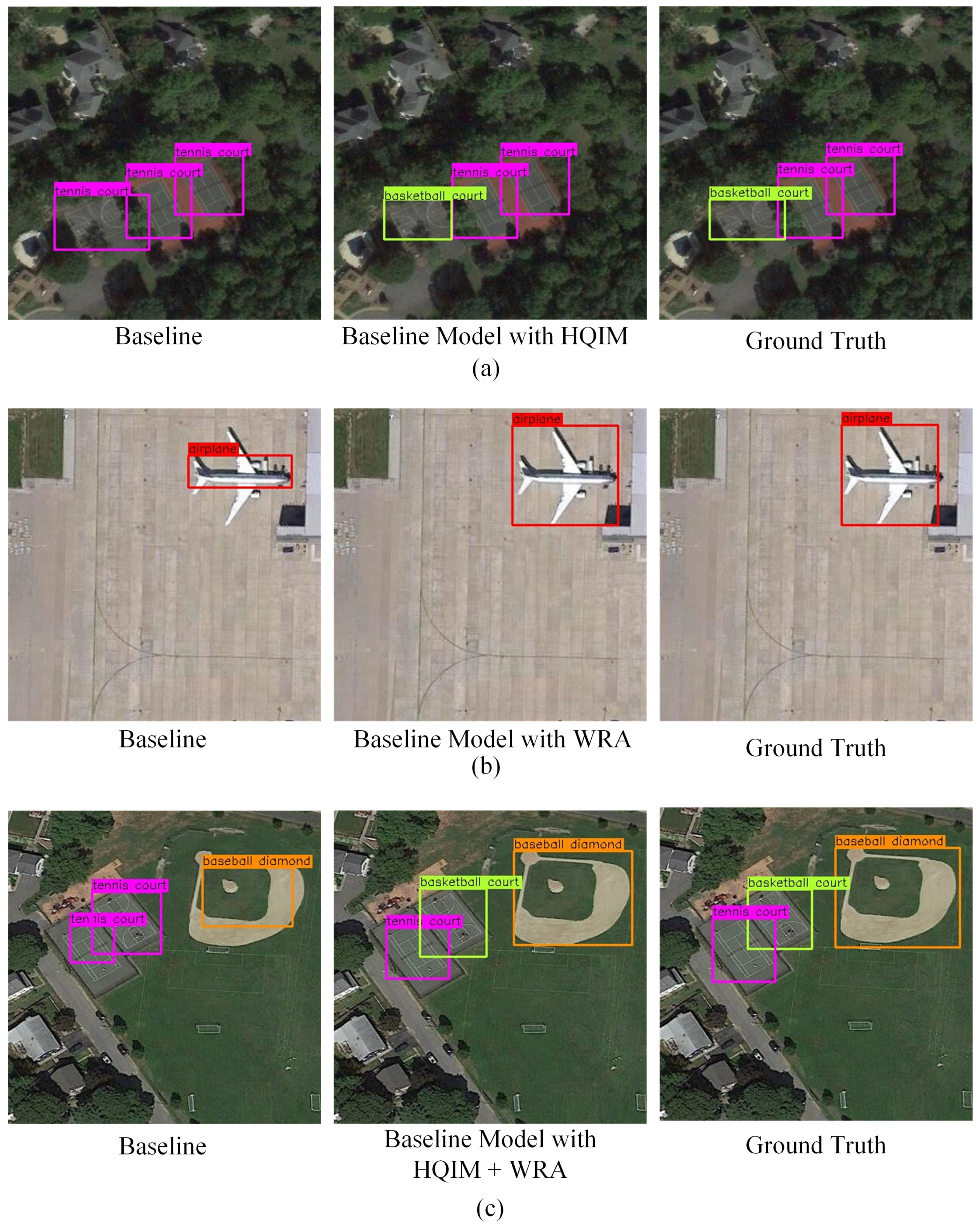
- During the label propagation process, the label of a neighboring instance is determined solely based on the spatial distance between it and its corresponding seed instance. Inevitably, this leads to some neighboring instances being misclassified. To address this issue, the HQIM module is proposed. This module utilizes feature similarity between seed instances and their neighboring instances to further refine the neighboring instances, thereby removing the misclassified neighboring instances.
- Most WSOD models often assign higher loss weights to instances focusing on the discriminative part of an object, compared with those covering the entire object. Consequently, they tend to detect the discriminative part of an object. To address this issue, we propose the WRA strategy, which exchanges the loss weights between these two types of instances.
2. Related Works
2.1. Weakly Supervised Deep Detection Network
2.2. Online Instance Classifier Refinement
2.3. Incorporating the Regression Branches into OICR
3. Proposed Method
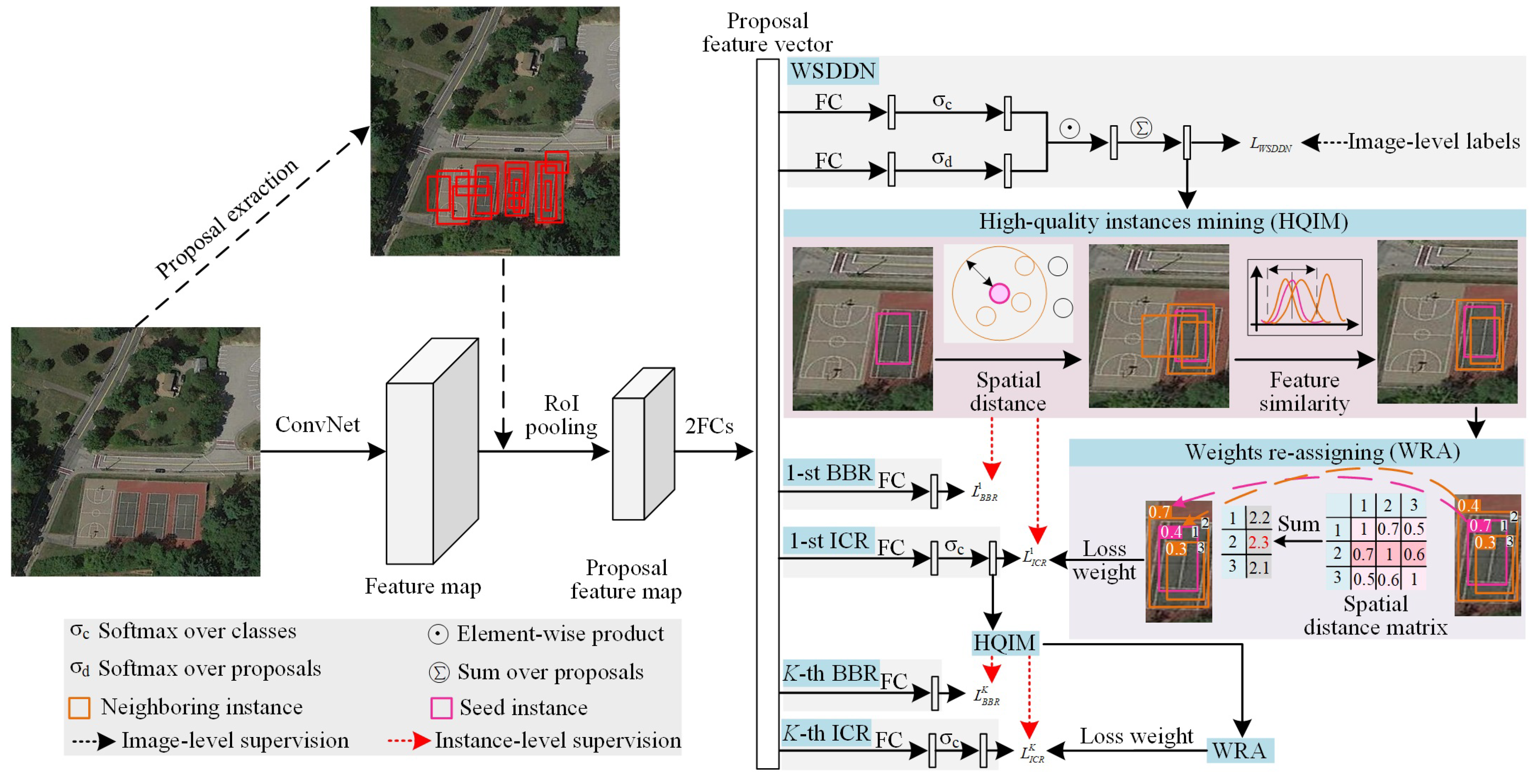
3.1. Overview
3.2. High-Quality Instance Mining Module
3.3. Weight Re-Assigning Strategy
3.4. Overall Training Loss
4. Materials, Data, and Experiments
4.1. Materials and Data
4.2. Experiments
4.2.1. Implementation Details
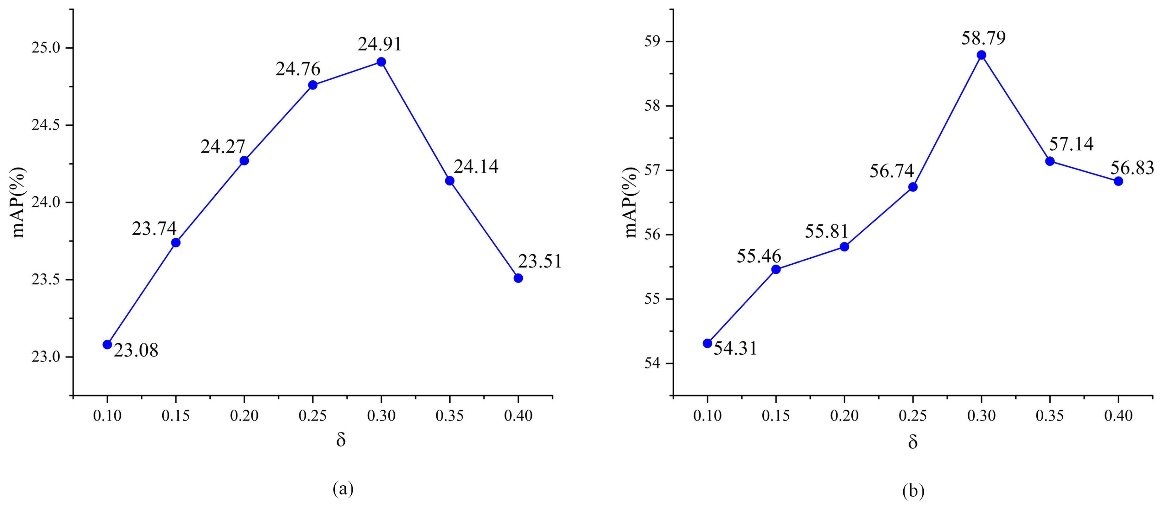
4.2.2. Parameter Analysis
4.2.3. Ablation Study
4.2.4. Quantitative Comparison with Popular Models
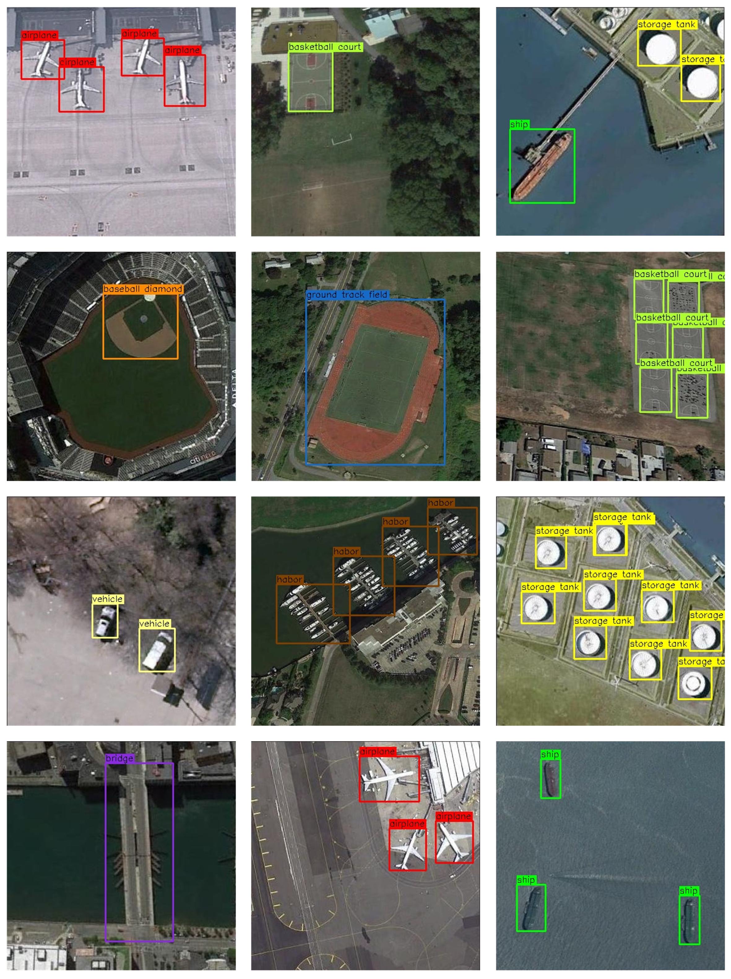
4.2.5. Subjective Evaluation
4.2.6. Evaluation of Computational Cost
5. Conclusions
Author Contributions
Funding
Data Availability Statement
Acknowledgments
Conflicts of Interest
Abbreviations
| WSOD | weak supervised object detection |
| RSI | remote sensing image |
| CS | class score |
| HQIM | high-quality instance mining |
| WRA | weight re-assigning |
References
- Girshick, R. Fast r-cnn. In Proceedings of the IEEE International Conference on Computer Vision (ICCV 2015), Santiago, Chile, 7–13 December 2015; pp. 1440–1448. [Google Scholar]
- Bilen, H.; Vedaldi, A. Weakly supervised deep detection networks. In Proceedings of the IEEE Conference on Computer Vision and Pattern Recognition (CVPR), Las Vegas, NV, USA, 27–30 June 2016; pp. 2846–2854. [Google Scholar]
- Cheng, G.; Han, J.; Lu, X. Remote Sensing Image Scene Classification: Benchmark and State of the Art. Proc. IEEE 2017, 105, 1865–1883. [Google Scholar] [CrossRef]
- Li, M.; Li, W.; Liu, Y.; Huang, Y.; Yang, G. Adaptive Mask Sampling and Manifold to Euclidean Subspace Learning with Distance Covariance Representation for Hyperspectral Image Classification. IEEE Trans. Geosci. Remote Sens. 2023, 61, 5508518. [Google Scholar] [CrossRef]
- Huo, Y.; Cheng, X.; Lin, S.; Zhang, M.; Wang, H. Memory-Augmented Autoencoder with Adaptive Reconstruction and Sample Attribution Mining for Hyperspectral Anomaly Detection. IEEE Trans. Geosci. Remote Sens. 2024, 62, 5518118. [Google Scholar] [CrossRef]
- Cheng, X.; Zhang, M.; Lin, S.; Zhou, K.; Zhao, S.; Wang, H. Two-Stream Isolation Forest Based on Deep Features for Hyperspectral Anomaly Detection. IEEE Geosci. Remote Sens. Lett. 2023, 20, 5504205. [Google Scholar] [CrossRef]
- Qian, X.; Zeng, Y.; Wang, W.; Zhang, Q. Co-Saliency Detection Guided by Group Weakly Supervised Learning. IEEE Trans. Multimed. 2023, 25, 1810–1818. [Google Scholar] [CrossRef]
- Cheng, X.; Huo, Y.; Lin, S.; Dong, Y.; Zhao, S.; Zhang, M.; Wang, H. Deep Feature Aggregation Network for Hyperspectral Anomaly Detection. IEEE Trans. Instrum. Meas. 2024, 73, 5033016. [Google Scholar] [CrossRef]
- Ren, S.; He, K.; Girshick, R.; Sun, J. Faster R-CNN: Towards real-time object detection with region proposal networks. IEEE Trans. Pattern Anal. Mach. Intell. 2016, 39, 1137–1149. [Google Scholar] [CrossRef] [PubMed]
- Qian, X.; Wu, B.; Cheng, G.; Yao, X.; Wang, W.; Han, J. Building a Bridge of Bounding Box Regression Between Oriented and Horizontal Object Detection in Remote Sensing Images. IEEE Trans. Geosci. Remote Sens. 2023, 61, 5605209. [Google Scholar] [CrossRef]
- Tang, P.; Wang, X.; Bai, X.; Liu, W. Multiple instance detection network with online instance classifier refinement. In Proceedings of the IEEE Conference on Computer Vision and Pattern Recognition (CVPR), Honolulu, HI, USA, 21 July–26 July 2017; pp. 2843–2851. [Google Scholar]
- Qian, X.; Li, C.; Wang, W.; Yao, X.; Cheng, G. Semantic segmentation guided pseudo label mining and instance re-detection for weakly supervised object detection in remote sensing images. Int. J. Appl. Earth Obs. Geoinf. 2023, 119, 103301. [Google Scholar] [CrossRef]
- Tang, P.; Wang, X.; Bai, S.; Shen, W.; Bai, X.; Liu, W.; Yuille, A. PCL: Proposal Cluster Learning for Weakly Supervised Object Detection. IEEE Trans. Pattern Anal. Mach. Intell. 2020, 42, 176–191. [Google Scholar] [CrossRef] [PubMed]
- Huang, Z.; Zou, Y.; Kumar, B.V.K.V.; Huang, D. Comprehensive Attention Self-Distillation for Weakly-Supervised Object Detection. In Proceedings of the Advances in Neural Information Processing Systems; Larochelle, H., Ranzato, M., Hadsell, R., Balcan, M., Lin, H., Eds.; Curran Associates, Inc.: Sydney, Australia, 2020; Volume 33, pp. 16797–16807. [Google Scholar]
- Wan, F.; Wei, P.; Jiao, J.; Han, Z.; Ye, Q. Min-entropy latent model for weakly supervised object detection. In Proceedings of the IEEE Conference on Computer Vision and Pattern Recognition (CVPR), Salt Lake City, UT, USA, 18–22 June 2018; pp. 1297–1306. [Google Scholar]
- Yao, X.; Feng, X.; Han, J.; Cheng, G.; Guo, L. Automatic weakly supervised object detection from high spatial resolution remote sensing images via dynamic curriculum learning. IEEE Trans. Geosci. Remote Sens. 2020, 59, 675–685. [Google Scholar] [CrossRef]
- Qian, X.; Wang, C.; Li, C.; Li, Z.; Zeng, L.; Wang, W.; Wu, Q. Multiscale Image Splitting Based Feature Enhancement and Instance Difficulty Aware Training for Weakly Supervised Object Detection in Remote Sensing Images. IEEE J. Sel. Top. Appl. Earth Obs. Remote Sens. 2023, 16, 7497–7506. [Google Scholar] [CrossRef]
- Huo, Y.; Qian, X.; Li, C.; Wang, W. Multiple Instance Complementary Detection and Difficulty Evaluation for Weakly Supervised Object Detection in Remote Sensing Image. IEEE Geosci. Remote Sens. Lett. 2023, 20, 6006505. [Google Scholar] [CrossRef]
- Feng, X.; Han, J.; Yao, X.; Cheng, G. Progressive contextual instance refinement for weakly supervised object detection in remote sensing images. IEEE Trans. Geosci. Remote Sens. 2020, 58, 8002–8012. [Google Scholar] [CrossRef]
- Qian, X.; Wang, C.; Wang, W.; Yao, X.; Cheng, G. Complete and Invariant Instance Classifier Refinement for Weakly Supervised Object Detection in Remote Sensing Images. IEEE Trans. Geosci. Remote Sens. 2024, 62, 5627713. [Google Scholar] [CrossRef]
- Seo, J.; Bae, W.; Sutherland, D.J.; Noh, J.; Kim, D. Object Discovery via Contrastive Learning for Weakly Supervised Object Detection. In Proceedings of the Computer Vision—ECCV 2022; Springer Nature: Cham, Switzerland, 2022; pp. 312–329. [Google Scholar]
- Cheng, G.; Xie, X.; Chen, W.; Feng, X.; Yao, X.; Han, J. Self-Guided Proposal Generation for Weakly Supervised Object Detection. IEEE Trans. Geosci. Remote Sens. 2022, 60, 5625311. [Google Scholar] [CrossRef]
- Xie, X.; Cheng, G.; Feng, X.; Yao, X.; Qian, X.; Han, J. Attention Erasing and Instance Sampling for Weakly Supervised Object Detection. IEEE Trans. Geosci. Remote Sens. 2024, 62, 5600910. [Google Scholar] [CrossRef]
- Ren, Z.; Yu, Z.; Yang, X.; Liu, M.Y.; Lee, Y.J.; Schwing, A.G.; Kautz, J. Instance-aware, context-focused, and memory-efficient weakly supervised object detection. In Proceedings of the IEEE/CVF Conference on Computer Vision and Pattern Recognition, Seattle, WA, USA, 13–19 June 2020; pp. 10598–10607. [Google Scholar]
- Qian, X.; Huo, Y.; Cheng, G.; Gao, C.; Yao, X.; Wang, W. Mining High-Quality Pseudoinstance Soft Labels for Weakly Supervised Object Detection in Remote Sensing Images. IEEE Trans. Geosci. Remote Sens. 2023, 61, 5607615. [Google Scholar] [CrossRef]
- Uijlings, J.R.; Van De Sande, K.E.; Gevers, T.; Smeulders, A.W. Selective search for object recognition. Int. J. Comput. Vis. 2013, 104, 154–171. [Google Scholar] [CrossRef]
- Cheng, G.; Zhou, P.; Han, J. Learning Rotation-Invariant Convolutional Neural Networks for Object Detection in VHR Optical Remote Sensing Images. IEEE Trans. Geosci. Remote Sens. 2016, 54, 7405–7415. [Google Scholar] [CrossRef]
- Li, K.; Cheng, G.; Bu, S.; You, X. Rotation-Insensitive and Context-Augmented Object Detection in Remote Sensing Images. IEEE Trans. Geosci. Remote Sens. 2018, 56, 2337–2348. [Google Scholar] [CrossRef]
- Cramer, M. The DGPF-Test on Digital Airborne Camera Evaluation Overview and Test Design. Photogramm.-Fernerkund.-Geoinf. 2010, 2010, 73–82. [Google Scholar] [CrossRef]
- Li, K.; Wan, G.; Cheng, G.; Meng, L.; Han, J. Object detection in optical remote sensing images: A survey and a new benchmark. ISPRS J. Photogramm. Remote Sens. 2020, 159, 296–307. [Google Scholar] [CrossRef]
- Everingham, M.; Van Gool, L.; Williams, C.K.I.; Winn, J.; Zisserman, A. The Pascal Visual Object Classes (VOC) Challenge. Int. J. Comput. Vis. 2010, 88, 303–338. [Google Scholar] [CrossRef]
- Simonyan, K.; Zisserman, A. Very deep convolutional networks for large-scale image recognition. arXiv 2014, arXiv:1409.1556. [Google Scholar]
- Krizhevsky, A.; Sutskever, I.; Hinton, G.E. ImageNet Classification with Deep Convolutional Neural Networks. In Proceedings of the Conference on Neural Information Processing Systems, Lake Tahoe, NV, USA, 3–6 December 2012; pp. 1097–1105. [Google Scholar]
- Hosang, J.; Benenson, R.; Schiele, B. Learning non-maximum suppression. In Proceedings of the IEEE Conference on Computer Vision and Pattern Recognition (CVPR), Honolulu, HI, USA, 21 July–26 July 2017; pp. 4507–4515. [Google Scholar]
- Feng, X.; Han, J.; Yao, X.; Cheng, G. TCANet: Triple Context-Aware Network for Weakly Supervised Object Detection in Remote Sensing Images. IEEE Trans. Geosci. Remote Sens. 2021, 59, 6946–6955. [Google Scholar] [CrossRef]
- Wang, B.; Zhao, Y.; Li, X. Multiple Instance Graph Learning for Weakly Supervised Remote Sensing Object Detection. IEEE Trans. Geosci. Remote Sens. 2022, 60, 5613112. [Google Scholar] [CrossRef]
- Feng, X.; Yao, X.; Cheng, G.; Han, J.; Han, J. SAENet: Self-Supervised Adversarial and Equivariant Network for Weakly Supervised Object Detection in Remote Sensing Images. IEEE Trans. Geosci. Remote Sens. 2022, 60, 5610411. [Google Scholar] [CrossRef]


| Baseline | HQIM | WRA | NWPU VHR-10.v2 | DIOR | ||
|---|---|---|---|---|---|---|
| mAP | CorLoc | mAP | CorLoc | |||
| 🗸 | 48.96 | 61.54 | 20.10 | 42.79 | ||
| 🗸 | 🗸 | 58.79 | 69.51 | 24.91 | 48.54 | |
| 🗸 | 🗸 | 61.51 | 72.94 | 27.23 | 50.89 | |
| 🗸 | 🗸 | 🗸 | 66.24 | 76.89 | 28.91 | 53.92 |
| Method | Airplane | Ship | Storage Tank | Baseball Diamond | Tennis Court | Basketball Court | Ground Track Field | Harbor | Bridge | Vehicle | mAP |
|---|---|---|---|---|---|---|---|---|---|---|---|
| Fast R-CNN [1] | 90.91 | 90.60 | 89.29 | 47.32 | 100.00 | 85.85 | 84.86 | 88.22 | 80.29 | 69.84 | 82.72 |
| Faster R-CNN [9] | 90.90 | 86.30 | 90.53 | 98.24 | 89.72 | 69.64 | 100.00 | 80.11 | 61.49 | 78.14 | 84.51 |
| WSDDN [2] | 30.08 | 41.72 | 35.98 | 88.90 | 12.86 | 23.85 | 99.43 | 13.94 | 1.92 | 3.60 | 35.12 |
| OICR [11] | 13.66 | 67.35 | 57.16 | 55.16 | 13.64 | 39.66 | 92.80 | 0.23 | 1.84 | 3.73 | 34.52 |
| MIST [24] | 69.69 | 49.16 | 48.55 | 80.91 | 27.08 | 79.85 | 91.34 | 46.99 | 8.29 | 13.36 | 51.52 |
| DCL [16] | 72.70 | 74.25 | 37.05 | 82.64 | 36.88 | 42.27 | 83.95 | 39.57 | 16.82 | 35.00 | 52.11 |
| PCIR [19] | 90.78 | 78.81 | 36.40 | 90.80 | 22.64 | 52.16 | 88.51 | 42.36 | 11.74 | 35.49 | 54.97 |
| MIG [36] | 88.69 | 71.61 | 75.17 | 94.19 | 37.45 | 47.68 | 100.00 | 27.27 | 8.33 | 9.06 | 55.95 |
| TCA [35] | 89.43 | 78.18 | 78.42 | 90.80 | 35.27 | 50.36 | 90.91 | 42.44 | 4.11 | 28.30 | 58.82 |
| SAE [37] | 82.91 | 74.47 | 50.20 | 96.74 | 55.66 | 72.94 | 100.00 | 36.46 | 6.33 | 31.89 | 60.76 |
| SPG [22] | 90.42 | 81.00 | 59.53 | 92.31 | 35.64 | 51.44 | 99.92 | 58.71 | 16.99 | 42.99 | 62.89 |
| PISLM [25] | 87.60 | 81.00 | 57.30 | 94.00 | 36.40 | 80.40 | 100.00 | 56.90 | 9.80 | 35.60 | 63.80 |
| SGPLM [12] | 90.70 | 79.90 | 69.30 | 97.50 | 41.60 | 77.50 | 100.00 | 44.40 | 17.20 | 33.50 | 65.20 |
| Ours | 90.81 | 80.52 | 73.42 | 96.59 | 47.35 | 78.94 | 100.00 | 43.89 | 18.35 | 33.51 | 66.24 |
| Method | Airplane | Ship | Storage Tank | Baseball Diamond | Tennis Court | Basketball Court | Ground Track Field | Harbor | Bridge | Vehicle | mAP |
|---|---|---|---|---|---|---|---|---|---|---|---|
| WSDDN [2] | 22.32 | 36.81 | 39.95 | 92.48 | 17.96 | 24.24 | 99.26 | 14.83 | 1.69 | 2.89 | 35.24 |
| OICR [11] | 29.41 | 83.33 | 20.51 | 81.76 | 40.85 | 32.08 | 86.60 | 7.41 | 3.70 | 14.44 | 40.01 |
| MIST [24] | 90.20 | 82.50 | 80.30 | 98.60 | 48.50 | 87.40 | 98.30 | 66.50 | 14.60 | 35.80 | 70.30 |
| DCL [16] | - | - | - | - | - | - | - | - | - | - | 69.70 |
| PCIR [19] | 100.00 | 93.06 | 64.10 | 99.32 | 64.79 | 79.25 | 89.69 | 62.96 | 13.26 | 52.22 | 71.87 |
| MIG [36] | 97.79 | 90.26 | 87.18 | 98.65 | 54.93 | 64.15 | 100.00 | 74.07 | 12.96 | 21.57 | 70.16 |
| TCA [35] | 96.91 | 91.78 | 95.13 | 88.65 | 66.90 | 62.83 | 95.98 | 54.18 | 19.63 | 55.50 | 72.76 |
| SAE [37] | 97.06 | 91.67 | 87.81 | 98.65 | 40.86 | 81.13 | 100.00 | 70.37 | 14.81 | 52.22 | 73.46 |
| SPG [22] | 98.06 | 92.67 | 70.08 | 99.65 | 51.86 | 80.12 | 96.20 | 72.44 | 12.99 | 60.02 | 73.41 |
| PISLM [25] | 94.40 | 86.60 | 68.50 | 97.80 | 69.80 | 87.50 | 100.00 | 68.60 | 16.00 | 56.60 | 74.60 |
| SGPLM [12] | 98.20 | 93.80 | 89.30 | 99.10 | 50.20 | 88.90 | 100.00 | 71.00 | 12.30 | 51.20 | 75.40 |
| Ours | 99.29 | 94.79 | 91.68 | 97.95 | 58.43 | 91.67 | 100.00 | 68.78 | 13.64 | 56.68 | 76.89 |
| Method | Airplane | Airport | Baseball Field | Basketball Court | Bridge | Chimney | Dam | Expressway Service Area | Expressway Toll Station | Golf Field | |
| Fast R-CNN [1] | 44.17 | 66.79 | 66.96 | 60.49 | 15.56 | 72.28 | 51.95 | 65.87 | 44.76 | 72.11 | |
| Faster R-CNN [9] | 50.28 | 62.60 | 66.04 | 80.88 | 28.80 | 68.17 | 47.26 | 58.51 | 48.06 | 60.44 | |
| WSDDN [2] | 9.06 | 39.68 | 37.81 | 20.16 | 0.25 | 12.28 | 0.57 | 0.65 | 11.88 | 4.90 | |
| OICR [11] | 8.70 | 28.26 | 44.05 | 18.22 | 1.30 | 20.15 | 0.09 | 0.65 | 29.89 | 13.80 | |
| MIST [24] | 32.01 | 39.87 | 62.71 | 28.97 | 7.46 | 12.87 | 0.31 | 5.14 | 17.38 | 51.02 | |
| DCL [16] | 20.89 | 22.70 | 54.21 | 11.50 | 6.03 | 61.01 | 0.09 | 1.07 | 31.01 | 30.87 | |
| PCIR [19] | 30.37 | 36.06 | 54.22 | 26.60 | 9.09 | 58.59 | 0.22 | 9.65 | 36.18 | 32.59 | |
| MIG [36] | 22.20 | 52.57 | 62.76 | 25.78 | 8.47 | 67.42 | 0.66 | 8.85 | 28.71 | 57.28 | |
| TCA [35] | 25.13 | 30.84 | 62.92 | 40.00 | 4.13 | 67.78 | 8.07 | 23.80 | 29.89 | 22.34 | |
| SAE [37] | 20.57 | 62.41 | 62.65 | 23.54 | 7.59 | 64.62 | 0.22 | 34.52 | 30.62 | 55.38 | |
| SPG [22] | 31.32 | 36.66 | 62.79 | 29.10 | 6.08 | 62.66 | 0.31 | 15.00 | 30.10 | 35.00 | |
| PISLM [25] | 29.10 | 49.80 | 70.90 | 41.40 | 7.20 | 45.50 | 0.20 | 35.40 | 36.80 | 60.80 | |
| SGPLM [12] | 39.10 | 64.60 | 64.40 | 26.90 | 6.30 | 62.30 | 0.90 | 12.20 | 26.30 | 55.30 | |
| Ours | 42.19 | 65.01 | 66.15 | 25.74 | 6.70 | 60.15 | 1.29 | 13.48 | 25.31 | 57.81 | |
| Method | Ground Track Field | Harbor | Overpass | Ship | Stadium | Storage Tank | Tennis Court | Train Station | Vehicle | Windmill | mAP |
| Fast R-CNN [1] | 62.93 | 46.18 | 38.03 | 32.13 | 70.98 | 35.04 | 58.27 | 37.91 | 19.20 | 38.10 | 49.98 |
| Faster R-CNN [9] | 67.00 | 43.86 | 46.87 | 58.48 | 52.37 | 42.35 | 79.52 | 48.02 | 34.77 | 65.44 | 55.49 |
| WSDDN [2] | 42.53 | 4.66 | 1.06 | 0.70 | 63.03 | 3.95 | 6.06 | 0.51 | 4.55 | 1.14 | 13.27 |
| OICR [11] | 57.39 | 10.66 | 11.06 | 9.09 | 59.29 | 7.10 | 0.68 | 0.14 | 9.09 | 0.41 | 16.50 |
| PCL [13] | 56.36 | 16.76 | 11.05 | 9.09 | 57.62 | 9.09 | 2.47 | 0.12 | 4.55 | 4.5 | 18.19 |
| MELM [15] | 41.05 | 26.12 | 0.43 | 9.09 | 8.28 | 15.02 | 20.57 | 9.81 | 0.04 | 0.53 | 18.65 |
| MIST [24] | 49.48 | 5.36 | 12.24 | 29.43 | 35.53 | 25.36 | 0.81 | 4.59 | 22.22 | 0.80 | 22.18 |
| DCL [16] | 56.45 | 5.05 | 2.65 | 9.09 | 63.65 | 9.09 | 10.36 | 0.02 | 7.27 | 0.79 | 20.19 |
| PCIR [19] | 58.51 | 8.60 | 21.63 | 12.09 | 64.28 | 9.09 | 13.62 | 0.30 | 9.09 | 7.52 | 24.92 |
| MIG [36] | 47.73 | 23.77 | 0.77 | 6.42 | 54.13 | 13.15 | 4.12 | 14.76 | 0.23 | 2.43 | 25.11 |
| TCA [35] | 53.85 | 24.84 | 11.06 | 9.09 | 46.40 | 13.74 | 30.98 | 1.47 | 9.09 | 1.00 | 25.82 |
| SAE [37] | 52.70 | 17.57 | 6.85 | 9.09 | 51.59 | 15.43 | 1.69 | 14.44 | 1.41 | 9.16 | 27.10 |
| SPG [22] | 48.02 | 27.11 | 12.00 | 10.02 | 60.04 | 15.10 | 21.00 | 9.92 | 3.15 | 0.06 | 25.77 |
| PISLM [25] | 48.50 | 14.00 | 25.10 | 18.50 | 48.90 | 11.70 | 11.90 | 3.50 | 11.30 | 1.70 | 28.60 |
| SGPLM [12] | 60.60 | 9.40 | 23.10 | 13.40 | 57.40 | 17.70 | 1.50 | 14.00 | 11.50 | 3.50 | 28.50 |
| Ours | 61.42 | 10.41 | 20.40 | 14.14 | 58.62 | 18.91 | 2.16 | 13.61 | 10.02 | 4.69 | 28.91 |
| Method | Airplane | Airport | Baseball Field | Basketball Court | Bridge | Chimney | Dam | Expressway Service Area | Expressway Toll Station | Golf Field | |
|---|---|---|---|---|---|---|---|---|---|---|---|
| WSDDN [2] | 5.72 | 59.88 | 94.24 | 55.94 | 4.92 | 23.40 | 1.03 | 6.79 | 44.52 | 12.75 | |
| OICR [11] | 15.98 | 51.45 | 94.77 | 55.79 | 2.63 | 23.89 | 0.00 | 4.82 | 56.68 | 22.42 | |
| MIST [24] | 91.60 | 53.20 | 93.50 | 66.30 | 10.80 | 30.70 | 1.50 | 14.03 | 35.20 | 47.50 | |
| DCL [16] | - | - | - | - | - | - | - | - | - | - | |
| PCIR [19] | 93.10 | 45.60 | 95.50 | 68.30 | 3.60 | 92.10 | 0.20 | 5.40 | 58.40 | 47.50 | |
| MIG [36] | 76.98 | 46.86 | 95.39 | 63.61 | 23.00 | 95.07 | 0.21 | 16.96 | 57.88 | 50.77 | |
| TCA [35] | 81.58 | 51.33 | 96.17 | 73.45 | 5.03 | 94.69 | 15.89 | 32.79 | 45.95 | 48.56 | |
| SAE [37] | 91.20 | 69.37 | 95.48 | 67.52 | 18.88 | 97.78 | 0.21 | 70.54 | 54.32 | 51.43 | |
| SPG [22] | 80.48 | 32.04 | 98.68 | 65.00 | 15.20 | 96.08 | 22.52 | 16.99 | 46.08 | 50.96 | |
| PISLM [25] | 85.50 | 68.90 | 96.80 | 75.80 | 11.60 | 94.70 | 0.80 | 67.50 | 60.50 | 46.50 | |
| SGPLM [12] | 92.20 | 58.30 | 97.80 | 74.20 | 16.20 | 95.20 | 0.30 | 51.30 | 56.20 | 52.30 | |
| Ours | 994.14 | 59.34 | 98.12 | 70.46 | 17.59 | 94.61 | 4.80 | 52.19 | 54.27 | 53.47 | |
| Method | Ground Track Field | Harbor | Overpass | Ship | Stadium | Storage Tank | Tennis Court | Train Station | Vehicle | Windmill | CorLoc |
| WSDDN [2] | 89.90 | 5.45 | 10.00 | 22.96 | 98.54 | 79.61 | 15.06 | 3.45 | 11.56 | 3.22 | 32.44 |
| OICR [11] | 91.41 | 18.18 | 18.70 | 31.80 | 98.28 | 81.29 | 7.45 | 1.22 | 15.83 | 1.98 | 34.77 |
| MIST [24] | 87.10 | 38.60 | 23.40 | 50.70 | 80.50 | 89.20 | 22.40 | 11.50 | 22.20 | 2.40 | 43.60 |
| DCL [16] | - | - | - | - | - | - | - | - | - | - | 42.20 |
| PCIR [19] | 88.60 | 15.80 | 5.20 | 39.50 | 98.10 | 85.60 | 13.40 | 56.50 | 9.70 | 0.60 | 46.10 |
| MIG [36] | 89.39 | 42.12 | 19.78 | 37.94 | 97.93 | 80.65 | 13.77 | 10.34 | 10.50 | 6.94 | 46.80 |
| TCA [35] | 85.26 | 38.91 | 20.17 | 30.63 | 84.59 | 91.46 | 56.28 | 3.79 | 10.45 | 1.25 | 48.41 |
| SAE [37] | 88.28 | 48.03 | 2.28 | 33.56 | 14.11 | 83.35 | 65.59 | 19.88 | 16.41 | 2.85 | 49.42 |
| SPG [22] | 89.18 | 49.45 | 22.00 | 35.16 | 98.61 | 90.04 | 32.56 | 12.73 | 9.98 | 2.34 | 48.30 |
| PISLM [25] | 75.20 | 50.50 | 28.30 | 39.70 | 92.60 | 77.00 | 55.10 | 10.10 | 20.90 | 5.60 | 53.20 |
| SGPLM [12] | 91.70 | 48.60 | 23.00 | 32.70 | 98.80 | 89.30 | 43.50 | 19.50 | 18.30 | 4.00 | 53.20 |
| Ours | 93.04 | 49.71 | 22.04 | 34.81 | 99.01 | 90.42 | 44.13 | 18.31 | 17.52 | 10.51 | 53.92 |
| Method | Training Time (H) | Inference Speed (fps) | GFLOPS (G) | mAP (%) |
|---|---|---|---|---|
| WSDDN [2] | 2.89 | 4.99 | 287.61 | 35.12 |
| OICR [11] | 3.25 | 4.15 | 286.23 | 34.52 |
| PCL [13] | 4.85 | 4.71 | 287.14 | 39.41 |
| MELM [15] | 5.12 | 4.79 | 290.34 | 42.29 |
| MIST [24] | 6.50 | 4.01 | 290.43 | 51.52 |
| PISLM [25] | 9.83 | 3.58 | 296.43 | 63.80 |
| SGPLM [12] | 10.50 | 4.21 | 334.26 | 65.20 |
| Ours | 4.12 | 4.93 | 289.93 | 66.24 |
Disclaimer/Publisher’s Note: The statements, opinions and data contained in all publications are solely those of the individual author(s) and contributor(s) and not of MDPI and/or the editor(s). MDPI and/or the editor(s) disclaim responsibility for any injury to people or property resulting from any ideas, methods, instructions or products referred to in the content. |
© 2024 by the authors. Licensee MDPI, Basel, Switzerland. This article is an open access article distributed under the terms and conditions of the Creative Commons Attribution (CC BY) license (https://creativecommons.org/licenses/by/4.0/).
Share and Cite
Xing, P.; Huang, M.; Wang, C.; Cao, Y. High-Quality Instance Mining and Weight Re-Assigning for Weakly Supervised Object Detection in Remote Sensing Images. Electronics 2024, 13, 4753. https://doi.org/10.3390/electronics13234753
Xing P, Huang M, Wang C, Cao Y. High-Quality Instance Mining and Weight Re-Assigning for Weakly Supervised Object Detection in Remote Sensing Images. Electronics. 2024; 13(23):4753. https://doi.org/10.3390/electronics13234753
Chicago/Turabian StyleXing, Peixu, Mengxing Huang, Chenhao Wang, and Yang Cao. 2024. "High-Quality Instance Mining and Weight Re-Assigning for Weakly Supervised Object Detection in Remote Sensing Images" Electronics 13, no. 23: 4753. https://doi.org/10.3390/electronics13234753
APA StyleXing, P., Huang, M., Wang, C., & Cao, Y. (2024). High-Quality Instance Mining and Weight Re-Assigning for Weakly Supervised Object Detection in Remote Sensing Images. Electronics, 13(23), 4753. https://doi.org/10.3390/electronics13234753